Weird scaling for 2-D avalanches:
Curing the faceting, and scaling in the lower critical dimension
Abstract
The non-equilibrium random-field Ising model is well studied, yet there are outstanding questions. In two dimensions, power law scaling approaches fail and the critical disorder is difficult to pin down. Additionally, the presence of faceting on the square lattice creates avalanches that are lattice dependent at small scales. We propose two methods which we find solve these issues. First, we perform large scale simulations on a Voronoi lattice to mitigate the effects of faceting. Secondly, the invariant arguments of the universal scaling functions necessary to perform scaling collapses can be directly determined using our recent normal form theory of the Renormalization Group. This method has proven useful in cleanly capturing the complex behavior which occurs in both the lower and upper critical dimensions of systems and here captures the 2D NE-RFIM behavior well. The obtained scaling collapses span over a range of a factor of ten in the disorder and a factor of in avalanche cutoff. They are consistent with a critical disorder at zero and with a lower critical dimension for the model equal to two.
We study the avalanche size distribution in the two-dimensional nucleated non-equilibrium random-field Ising model (NE-RFIM), simulated on a Voronoi lattice to bypass faceting, and analyzed using the scaling predictions of the nonlinear renormalization-group flows predicted for the lower critical dimension. We find excellent agreement over a large critical region, addressing several outstanding issues in the field.
The NE-RFIM is perhaps the best-understood model of crackling noise Sethna et al. 2001, exhibiting power-law distributions of avalanche sizes at a critical disorder representing the standard deviation of the strength of the random field at each site. The model transitions from a ‘down-spin’ state to an ‘up-spin’ state as an external field increases. Above the critical disorder , this transition is composed of avalanches of spins of size limited by a typical cutoff ; below the critical disorder a finite fraction of the spins flip in a single event, with precursors and aftershock sizes limited by . This model, albeit simple, contains the necessary ingredients to describe hysteretic and avalanche behaviors in a diverse set of systems. Barkhausen noise in magnets Bertotti 1998 decision making in socio-economics Bouchaud 2013, absorption and desorption in superfluids Lilly et al. 1996; Detcheverry et al. 2004 as well as the effects of nematicity in high superconductors Bonetti et al. 2004; Carlson et al. 2006; Phillabaum and Dahmen 2012 can each be understood in terms of ‘crackling noise’ naturally described by the NE-RFIM.
Although the NE-RFIM itself has been around in various forms since the 1970s Imry and Ma 1975, there are still a number of current questions and issues:
Is it in the same universality class as the equilibrium RFIM model Balog et al. 2018? It has long been debated whether the equilibrium and non-equilibrium versions of the model are in the same universality class. This question of universality has been approached in a number of ways which have suggested the same class for the two models Maritan et al. 1994; Pérez-Reche and Vives 2004; Colaiori et al. 2004; Liu and Dahmen 2009a; Liu and Dahmen 2009b; Balog et al. 2014. Recent work using the non-perturbative RG indicate that the two models are in different universality classes in lower dimensions Balog et al. 2018. Our findings pretty clearly imply they are also different in two dimensions.
Is the lower critical dimension (LCD) two, or is power law scaling sufficient to capture the behavior in ? The equilibrium RFIM has been shown to have a LCD equal to two Bray and Moore 1985, and the same is believed to be true for the front-propagation variant of the NE-RFIM Drossel and Dahmen 1998. For the nucleated model we study here, some suggest that the LCD is two Perković et al. 1995; Perković et al. 1996, others suggest that power-laws are indeed able to capture the behavior and no crossover occurs in 2D Spasojević et al. 2011a; Spasojević et al. 2011b, and some suggest that a lower critical dimension does not exist for this model Thongjaomayum and Shukla 2013; Kurbah et al. 2015; Shukla and Thongjaomayum 2016; Shukla and Thongjaomayum 2017. Here, we derive the expected non-power-law scaling in the LCD from a nonlinear renormalization-group analysis, and find excellent agreement with the data presuming an LCD of two, while power-law scaling fails to capture the behavior.
Is the value of the critical disorder in zero, or positive? In the nucleated model, the critical disorder appears to decrease with dimension, going from in 5D to in 3D Sethna et al. 2004. This behavior in conjunction with the observation that for both the equilibrium and front-propagation problems, is found to be zero Drossel and Dahmen 1998 suggests that may be quite small. Early work on the nucleated model, presuming power law scaling Vives et al. 1995; Perković et al. 1996; Kuntz 1999, yielded positive Vives et al. 1995, but more recent work on larger systems finds a smaller Spasojević et al. 2011a; Spasojević et al. 2011b collapsing over a small range . Our non-power-law scaling form would predict that power-law fits at a given system size should succeed in small ranges of disorder, but that larger system sizes will yield lower and lower predicted critical disorders. Our results are compatible with a critical disorder of zero, directly (random field strength ) or perhaps more naturally in conjunction with some random bond disorder (so , see Appendix B.2).
Scaling collapses (e.g. Figs 3 and 4) are the gold standard for identifying universal scaling behavior at critical points. Commonly used in simulations and experiments, the scaling form for a function of two variables usually becomes a power law times a universal function of the ratio of two power laws – a result which follows from linearizing the renormalization-group (RG) flows. The LCD, however, is precisely the dimension at which one of the eigenvalues of the RG flow vanishes and the nonlinear terms become crucial to the behavior. Recently, Raju et al. Raju et al. 2019 analyzed non-linearities in renormalization group flows using normal form theory drawn from the dynamical systems community. In the cases for which power laws work well, the dynamics are governed by a hyperbolic fixed point which can be linearized by a change of variables, leading to traditional scaling predictions. Our simulations indicate that the LCD for the NE-RFIM is poised at a transcritical bifurcation in the RG flow. By considering the form the flow equations should take, we are able to provide concrete non-power-law invariant scaling variables which enable collapse of our data over a range of a factor of ten in the disorder. This success, and the enormous critical region, suggests that using the appropriate invariant scaling variables can be effective for analyzing experiments and simulations systems at their LCD (like the XY model), despite exponentially growing correlation lengths. (Similar analyses have been done for the 4-state Potts model Salas and Sokal 1997 and the XY model Pelissetto and Vicari 2013, except that their invariant scaling variables include only their predicted leading log corrections.)
In addition to the application of our normal form theory of the Renomalization Group, another key component to the success of our collapses is an approach to dealing with the faceting. Running simulations on a square lattice leads to distortions in the shape of the distributions of interest due to lattice effects as the critical point is approached. Long, unnaturally straight avalanche boundaries for small disorder arise which serve to effectively decrease the simulation size (Appendix B.1). To combat this, we run our simulations on a Voronoi lattice. Although this introduces some intrinsic disorder (Appendix B.2), we find the Voronoi lattice to be effective in combating faceting effects, enabling clean collapses over a range of a factor of ten in the disorder, a significantly larger range than the current available collapses which use data in a range .
The paper is organized as follows. In Section I, we define the model we will use in detail. In Section II.1, we work out the normal form of the RG flows. In Section II.2, we derive the invariant scaling combinations used for the scaling collapses. We discuss the efficacy of our scaling collapses, our ability to fit parameters and alternative choices of scaling forms in Section III before concluding.
I Model definition


The non-equilibrium random-field Ising model (NE-RFIM) consists of Ising spins connected by bonds of strength , subject both to a random field and an external field :
| (1) |
The external field starts at and grows until all spins have flipped from to . The spins flip when they can decrease the energy , triggered either by an increase in the external field (spawning a new avalanche), or by being kicked by the spin flip of a neighbor (propagating an existing avalanche). The random fields are chosen from a distribution with zero mean and a width describing the strength of the disorder from the random field. The simulations in this work use the traditional Gaussian form for the disorder, . At large disorder the avalanches are all small; as the disorder decreases the avalanches grow in size (Fig. 1). Avalanche size is denoted by . There are two different variants of the NE-RFIM. The one we study is ‘nucleated’ – all spins start pointing down (-1), and the first avalanche is triggered by a spin with an unusually large positive random field . Another model, inspired by fluid invasion into porous media, has a pre-existing front (e.g. a line of fluid-filled spins at the bottom), and does not allow for spins to flip unless at least one neighbor is up (i.e., with a path allowing fluid to enter). We study the nucleated model, but occasionally refer to results from the front propagation model.
Our simulations differ from tradition in that our spins are not on a regular lattice. We work in two dimensions (where the behavior is still controversial), but do not simulate spins on a square lattice but rather, as mentioned earlier, on a Voronoi lattice (Fig. 2) – with randomly scattered spins interacting with nearest neighbors. The neighbors are determined by shared boundaries of Voronoi cells for each spin. The spin’s Voronoi cell is the set of points on the plane nearest to that spin.
II Renormalization Group Analysis
II.1 Flow equations
Following the convention of Bray and Moore Bray and Moore 1985 for the equilibrium model, we define a parameter which corresponds to the ratio of the disorder over the coupling and determine its RG flow equation through symmetry considerations. In principle, there are an infinite series of terms. Using only analytic changes of variables, however, it is possible to remove all terms of or higher without removing any universal behavior Raju et al. 2019. We give a brief version of the argument here for completeness.
In the equilibrium model, the flow equation is found to be where and Bray and Moore 1985. For the NE-RFIM, however, has the symmetry while lacks this symmetry due to the external field. This implies and suggests that the RG flow for in the NE-RFIM must include a squared order term. (Note that the symmetry for the equilibrium Hamiltonian is only valid for systems with a bipartite lattice. It would be natural to test whether the equilibrium RFIM on a triangular lattice retains the pitchfork form or changes to the transcritical divergence as suggested by our symmetry argument.)
Assuming the lower critical dimension , we have , and may choose a scale for the disorder such that the prefactor of the squared order term in the flow equation of is equal to one. Taking , the choice we make for is where defines the critical disorder. The generic form for the flow equation of is given by
| (2) |
Given such a flow equation with an infinite number of possible terms, normal form theory proceeds by systematically removing higher order terms with a change of variables. Consider the change of variables The resulting flow equation takes the form:
| (3) |
With an appropriate choice of and , the coefficient of may easily be set to zero. Likewise, all higher order terms may be systematically removed. Dropping the tildes and subscripts for clarity, the final form of the flow equation is given by
| (4) |
which corresponds to the normal form of a transcritical bifurcation 11 1 The traditional transcritical bifurcation normal form Strogatz 2014 is derived using the implicit function theorem, but involves changes of variables that alter critical properties in singular ways. Eq. 4 is the simplest form that can be reached by successive polynomial changes of variables..
Next consider the flow equations for and . The eigenvalues for these are given by and respectively where denotes the fractal dimension. In each case, the zero eigenvalue of gives rise to cross terms between and and and . Again, in principle, we have an infinite number of possible terms but most all terms may be removed with a polynomial change of variables. The flow equations for and are hence given by
| (5) |
where in higher dimensions and . In two dimensions, the individual exponents and and , keeping the combinations we use finite. The coefficients , , and are universal. Just as the linear terms at ordinary (hyperbolic) fixed points yield universal critical exponents, these terms control universal dependences of physical behavior with changes in the control parameters. Note that, while they cannot be set to zero by a coordinate change, they may have universal values equal to zero 22 2 For example, a term corresponding to in the flow equations of the magnetic field turns out to be equal to zero in the 4-d Ising model.
II.2 Invariant Scaling combinations
The appropriate scaling variables to collapse the data can be directly calculated from the flow equations (see Appendix A for full derivation). We may directly solve for the correlation length in the normal form variables by integrating Eq. 4. The invariant scaling combination for obtained takes the form where is a nonlinear function of . We allow for an undetermined scale factor . The resulting form is given by
| (6) |
Likewise for , we obtain:
| (7) |
where is invariant under the RG, and is another scale factor.
First consider the area weighted size distribution . In analogy with three dimensions, we take where is the scaling variable and the prefactor of arises from normalization constraints with from Equation 6. The avalanche size distribution also depends on an unknown universal scaling function, . In order to perform our fits, we choose functional forms for the universal scaling functions. For the area weighted avalanche size distribution, we choose
| (8) |
where the leading power law has been absorbed into here and is the normalization factor where denotes the regularized upper incomplete gamma function. The associated collapse is shown in Figure 3. The best-fit values of the fitting parameters are and , which yield an approximation to the universal scaling function (Fig. 3).
Likewise, in analogy with three dimensions, we obtain where is the invariant scaling variable. For we choose
| (9) |
where , and is a normalization factor computed as a sum of over the data range. The associated collapse is shown in Figure 4. The best-fit values of the fitting parameters are , , , and , approximating our prediction for the universal scaling function (Fig. 4).


III Parameter values
Through performing the scaling collapses we are provided with values of and for each value of disorder, . Using the nonlinear scaling forms for each of these we may then extract values for the associated parameters. An unconstrained fit yields a fractal dimension larger than two, the dimension of the system, which is unphysical. The 2D avalanches we consider appear compact. This suggests that the fractal dimension should be given by and that the maximum avalanche size should scale as the square of the correlation length. For this reason, we expect also that and set . Imposing these constraints, the fits obtained are able to describe the data well, as shown in Figure 5.
As usual, our data is precise enough that the statistical errors in the parameters we estimate are small compared to various systematic errors. The dependence of our estimated and on the range of data and functional form appear smaller than the datapoints in Fig. 5. We explore the importance of finite size effects and lattice effects at small and large by performing the collapses and subsequent fits of the nonlinear forms using subsets of the disorders for which we have data [11 out of 13 points]. The best-fit parameters, with error estimates given by the standard deviation of these measurements, are given in the NF column of Table 1. Even larger uncertainties, estimated in the last column, arise from excellent fits that test various conjectures about the parameters.
Note that the best fit value of is found to be less than zero. There are several possible explanations for this. One, could indicate the Voronoi lattice used introduces an amount of intrinsic disorder(Appendix B.2). This is certainly plausible as random bond and random field disorder are expected to belong to the same universality class Dahmen and Sethna 1996; Vives et al. 1995. Alternatively, constraining we obtain a comparable fit by including an alternative normal form, , differing from and by analytic corrections to scaling (expected for the larger disorders considered, see Appendix A.3). In either case, the results are consistent with
| Conjecture | |||||
|---|---|---|---|---|---|
| 0 | 0 | ||||
| 1 | |||||
| 0 | 0 | 0 | 0 | ||
| 2 | 2 | 2 | 2 | 2 |
As a test of our finding that the 2D NE-RFIM corresponds to a transcitical bifurcation, we may compare the fits obtained to those using different underlying assumptions. In particular, it is straightforward to calculate and assuming a hyperbolic fixed point (corresponding to power law scaling) and a pitchfork bifurcation (Appendix A.4). For each of these cases we can perform a fit to the values of and extracted from the collapse. The comparison of these fits are shown in Figure 5.

It is particulary illuminating to consider the behavior of . For a transcritical bifurcation, the exponential divergence (ignoring and in Equation 6) gives Hence, if the behavior corresponds to a transcritical bifurcation, we would expect a plot of to scale linearly with the disorder. A comparison of the linear fit to , along with the plots of for the best fits with a power law and pitchfork form are shown in Figure 6.
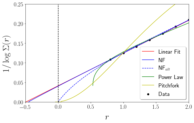
The results clearly support a transcritical bifurcation, perhaps with (Appendix B.2), and challenge the alternative power law and pitchfork assumptions.
Simulation data of the 2D non-equilibrium random-field Ising model on a lattice which suppresses faceting is explained well by the presence of a transcritical bifurcation, and is incompatible with power law scaling or pitchfork normal forms without large corrections to scaling. This provides evidence that (1) the universality class of the equilibrium and non-equilibrium models are indeed different and that (2) power law scaling (which is governed by a hyperbolic fixed point) is not the correct approach for this system in this regime. The latter conclusion, in turn, is consistent with (3) the LCD of the model being equal to two, or perhaps close to two.
Although the transcitical bifurcation provides the best description of our simulation data, the corresponding parameter values are difficult to pin down. There are a number of restrictions we can make to the parameter values and still obtain a reasonable joint fit of and For example, we may require that the Harris criteria saturates, that Perković et al. 1996 or that the coefficient of the quintic order term . Each of these provides a good description of our data. A wide range of fits with various restrictions are shown in Figures 7, 8, 9, and 10. Corresponding best fit parameter values are shown in Tables 3 and 3. As anticipated, the alternative form for the transcritical bifurcation is able to better capture the behavior far from the critical point.


| 0 | 0 | |||||||
| 2 | 2 | 2 | 2 | 2 | 2 | 2 | 2 | |
| 1 | 1 | 1 | 1 | |||||
| 0 | 0 | |||||||
| 0 | 0 | 0 | 0 | 0 | ||||
| 0 | 0 |
| 0 | |||||||
|---|---|---|---|---|---|---|---|
| 2 | 2 | 2 | 2 | 2 | 2 | 2 | |
| 1 | 1 | 1 | 1 | ||||
| 0 | 0 | ||||||
| 0 | 0 | 0 | 0 | 0 | |||
| 0 | 0 |
In three and higher dimensions Perković et al. 1996; Kuntz and Sethna 2000, measuring a variety of avalanche properties was crucial in pinning down the universal critical exponents and scaling functions. and the cumulative avalanche size distribution, measured here, were supplemented by measurements of finite-size scaling, avalanche correlation functions, avalanche sizes binned in , spanning avalanches, avalanche durations, and average avalanche temporal shapes. Larger system sizes should be possible with improved Voronoi data structures: the intercept of Fig. 6 suggests that a random-field free simulation of size might divide into multiple avalanches at , implying that .
IV Conclusions
In summation, performing large scale simulations on a Voronoi lattice and analyzing the RG flow equations yields valuable insight into the behavior of the NE-RFIM in 2D. The data collapses in a range of a factor of ten in the disorder and a factor of in the avalanche cutoff. The scaling is consistent with a critical disorder of zero and with a lower critical dimension of two.
Acknowledgements.
This work was partially supported by NSF grants DMR-1719490 and DGE-1144153. AR acknowledges support from the Simons Foundation. We thank A. Alan Middleton, Gilles Tarjus, and Karin A. Dahmen for helpful discussions.References
- Sethna et al. (2001) J. P. Sethna, K. A. Dahmen, and C. R. Myers, Nature 410, 242 (2001).
- Bertotti (1998) G. Bertotti, Hysteresis in Magnetism (Academic, New York, 1998).
- Bouchaud (2013) J.-P. Bouchaud, J. Stat. Phys. 151, 567 (2013).
- Lilly et al. (1996) M. P. Lilly, A. H. Wootters, and R. B. Hallock, Phys. Rev. Lett. 77, 4222 (1996).
- Detcheverry et al. (2004) F. Detcheverry, E. Kierlik, M. L. Rosinberg, and G. Tarjus, Langmuir 20, 8006 (2004).
- Bonetti et al. (2004) J. A. Bonetti, D. S. Caplan, D. J. Van Harlingen, and M. B. Weissman, Phys. Rev. Lett. 93, 087002 (2004).
- Carlson et al. (2006) E. W. Carlson, K. A. Dahmen, E. Fradkin, and S. A. Kivelson, Phys. Rev. Lett. 96, 097003 (2006).
- Phillabaum and Dahmen (2012) E. W. Phillabaum, B.and Carlson and K. A. Dahmen, Nature Communications 3, 915 EP (2012).
- Imry and Ma (1975) Y. Imry and S.-k. Ma, Phys. Rev. Lett. 35, 1399 (1975).
- Balog et al. (2018) I. Balog, G. Tarjus, and M. Tissier, Phys. Rev. B 97, 094204 (2018).
- Maritan et al. (1994) A. Maritan, M. Cieplak, M. R. Swift, and J. R. Banavar, Phys. Rev. Lett. 72, 946 (1994).
- Pérez-Reche and Vives (2004) F. J. Pérez-Reche and E. Vives, Phys. Rev. B 70, 214422 (2004).
- Colaiori et al. (2004) F. Colaiori, M. J. Alava, G. Durin, A. Magni, and S. Zapperi, Phys. Rev. Lett. 92, 257203 (2004).
- Liu and Dahmen (2009a) Y. Liu and K. A. Dahmen, Europhys. Lett. 86, 56003 (2009a).
- Liu and Dahmen (2009b) Y. Liu and K. A. Dahmen, Phys. Rev. E 79, 061124 (2009b).
- Balog et al. (2014) I. Balog, M. Tissier, and G. Tarjus, Phys. Rev. B 89, 104201 (2014).
- Bray and Moore (1985) A. J. Bray and M. A. Moore, J. Phys. C: Solid State Physics 18, L927 (1985).
- Drossel and Dahmen (1998) B. Drossel and K. Dahmen, Eur. Phys. J. B 3, 485 (1998).
- Perković et al. (1995) O. Perković, K. Dahmen, and J. P. Sethna, Phys. Rev. Lett. 75, 4528 (1995).
- Perković et al. (1996) O. Perković, K. Dahmen, and J. P. Sethna, arXiv:cond-mat/9609072 (1996).
- Spasojević et al. (2011a) D. Spasojević, S. Janićević, and M. Knežević, Phys. Rev. Lett. 106, 175701 (2011a).
- Spasojević et al. (2011b) D. Spasojević, S. Janićević, and M. Knežević, Phys. Rev. E 84, 051119 (2011b).
- Thongjaomayum and Shukla (2013) D. Thongjaomayum and P. Shukla, Phys. Rev. E 88, 042138 (2013).
- Kurbah et al. (2015) L. Kurbah, D. Thongjaomayum, and P. Shukla, Phys. Rev. E 91, 012131 (2015).
- Shukla and Thongjaomayum (2016) P. Shukla and D. Thongjaomayum, J. Phys. A: Mathematical and Theoretical 49, 235001 (2016).
- Shukla and Thongjaomayum (2017) P. Shukla and D. Thongjaomayum, Phys. Rev. E 95, 042109 (2017).
- Sethna et al. (2004) J. P. Sethna, K. A. Dahmen, and O. Perkovic, arXiv:cond-mat/0406320 (2004).
- Vives et al. (1995) E. Vives, J. Goicoechea, J. Ortín, and A. Planes, Phys. Rev. E 52, R5 (1995).
- Kuntz (1999) M. C. Kuntz, Ph.D. thesis, Cornell University (1999).
- Raju et al. (2019) A. Raju, C. B. Clement, L. X. Hayden, J. P. Kent-Dobias, D. B. Liarte, D. Z. Rocklin, and J. P. Sethna, Phys. Rev. X 9, 021014 (2019).
- Salas and Sokal (1997) J. Salas and A. D. Sokal, Journal of Statistical Physics 88, 567 (1997).
- Pelissetto and Vicari (2013) A. Pelissetto and E. Vicari, Phys. Rev. E 87, 032105 (2013).
- (33) The traditional transcritical bifurcation normal form Strogatz 2014 is derived using the implicit function theorem, but involves changes of variables that alter critical properties in singular ways. Eq. 4 is the simplest form that can be reached by successive polynomial changes of variables.
- (34) For example, a term corresponding to in the flow equations of the magnetic field turns out to be equal to zero in the 4-d Ising model.
- Dahmen and Sethna (1996) K. Dahmen and J. P. Sethna, Phys. Rev. B 53, 14872 (1996).
- Kuntz and Sethna (2000) M. C. Kuntz and J. P. Sethna, Phys. Rev. B 62 (2000).
- Strogatz (2014) S. Strogatz, Nonlinear Dynamics and Chaos: With Applications to Physics, Biology, Chemistry, and Engineering, Studies in Nonlinearity (Avalon Publishing, 2014).
- Rycroft (2009) C. H. Rycroft, Chaos 19, 041111 (2009).
- Chen et al. (2011) Y. J. Chen, S. Papanikolaou, J. Sethna, S. Zapperi, and G. Durin, Phys. Rev. E 84, 061103 (2011).
- Meakin (1986) P. Meakin, Phys. Rev. A 33, 3371 (1986).
- Meakin et al. (1987) P. Meakin, R. C. Ball, P. Ramanlal, and L. M. Sander, Phys. Rev. A 35, 5233 (1987).
- Blossey et al. (1998) R. Blossey, T. Kinoshita, and J. Dupont-Roc, Physica A: Statistical Mechanics and its Applications 248, 247 (1998).
- Brakke (2005) K. A. Brakke, “200,000,000 random voronoi polygons,” (2005).
- Dhar et al. (1997) D. Dhar, P. Shukla, and J. P. Sethna, Journal Of Physics A-Mathematical And General 30, 5259 (1997).
Appendix A Invariant Scaling Combinations
A.1 Power Law Form
As our invariant parameter combinations are unorthodox, we provide here a thorough derivation and a comparison to the usual power law ‘homogeneous’ variables seen at the usual hyperbolic fixed points. The invariant scaling combinations corresponding to traditional power law scaling may be simply derived from the flow equations in 3 and higher dimensions. We have
| (10) |
Taking and integrating gives
| (11) |
Performing the integral and working through the algebra
| (12) |
where corresponds to the fixed point of the RG and is hence a constant. The invariant scaling combination in this instance is thus
| (13) |
which agrees with the results in 3 and higher dimensions Perković et al. 1996. Similarly for we have
| (14) |
Performing the integral and working through the algebra
| (15) |
The invariant scaling combination is hence
| (16) |
which again agrees with the literature Perković et al. 1996.
A.2 Transcritical Form
The flow equations using the transcritical form for the disorder are as follows
| (17) |
As before, we take the integral of over and obtain
| (18) |
Solving for we have
| (19) |
where denotes a function of and and is therefore constant. The invariant scaling combination in this case is then
| (20) |
where
| (21) |
Likewise for we obtain an invariant scaling combination
| (22) |
where
| (23) |
A.3 Alternative Transcritical Form
Applying our methods to the 2D equilibrium RFIM, we find that the fixed point is given by a pitchfork bifurcation corresponding to
| (24) |
In this instance, however, the behavior of the correlation length suggests an alternative choice for the normal form
| (25) |
as discussed in Raju et al. 2019. This form, while retaining the pitchfork behavior, produces a well behaved correlation function that is also able to capture higher order corrections to scaling which we expect to become important further from the critical point. We may apply the same procedure in the non-equilibrium case, although the function for the correlation length here appears well behaved. This yields an alternative form for the transcritical bifurcation given by
| (26) |
We can integrate the first equation to a final point to find the divergence of the correlation length :
| (27) |
| (28) | ||||
| (29) |
As before, to determine , we take the integral of over and obtain
| (30) |
Solving for we have
| (31) |
where denotes a function of and and is therefore constant. The invariant scaling combination in this case is then
| (32) |
where
| (33) |
Likewise for we obtain an invariant scaling combination
| (34) |
where
| (35) |
A.4 Pitchfork Form
The flow equations using a pitchfork form for the disorder are as follows
| (36) |
As before, we take the integral of over and obtain
| (37) |
Solving for we have
| (38) |
The invariant scaling combination in this case is then
| (39) |
where
| (40) |
Likewise for we obtain an invariant scaling combination
| (41) |
where
| (42) |
Appendix B Simulations
Experience simulating the RFIM on a square lattice has revealed a propensity for faceting in which the shape of the avalanche size distribution becomes dependent on properties of the lattice for small avalanche sizes. To mitigate this effect, we perform simulations on a periodic Voronoi lattice (Fig. 2) where, for each value of , we consider 100 distinct lattices of size 1000x1000. Voronoi cells were chosen by generating random coordinates between 0 and 1 and constructing the cells with a 2D implementation of Voro++ Rycroft 2009 provided by C. H. Rycroft. Examples of the avalanche behavior for different values of are shown in Figure 1.
We note that much larger simulations have been done on the square lattice, including a thorough analysis of results from a lattice Spasojević et al. 2011a; Spasojević et al. 2011b. In analysis of in house simulations on a square lattice, however, we encountered long, unnaturally straight avalanche boundaries. We found these distortions strongly affected the shape of the size distribution for small disorders and served to effectively decreased the system size, a difficulty which became dramatically more pronounced as the disorder decreased. In addition to lattice dependent effects infecting the distributions for larger and larger avalanche sizes approaching the critical point, this effective reduction of system size encouraged the use of a Voronoi lattice.
From the simulations we extract two quantities of interest: the area weighted avalanche size distribution Chen et al. 2011 and the change in magnetization of the sample with respect to the field . Alternatively, we may write these as and where is a function of as defined earlier.
Lattice effects are a major feature in the two-dimensional NE-RFIM. On the square lattice, the strong faceting effects due to the lattice distorted the avalanche size distribution, effectively giving a short-distance cutoff not of the lattice constant, but of the typical length of the straight, horizontal or vertical portions of the avalanche boundaries. On the random Voronoi lattices we simulate, the stochastic bond configurations introduce a randomness in the connectivity of the network, which we argue here may lead to an effective disorder that does not vanish even as . One could envision off-lattice simulations or experiments that could bypass these effects. Here, instead, we shall briefly explore the faceting and intrinsic disorder, and speculate about strategies one might use to minimize their effects.
B.1 Faceting
The experimental systems to which we apply our avalanche model typically do not have an important underlying lattice anisotropy. The length scales of the domain wall pinning and avalanches are typically much larger than the atomic scale, and the materials are often amorphous or polycrystalline. We thus do not want an underlying crystalline lattice dominate the behavior on long length scales.
Often there are emergent symmetries at critical points. Lattice models (Ising, QCD) break rotational symmetry, but the emergent fluctuations on long length scales restore this symmetry – the symmetry of the fixed point is greater than that of the Hamiltonian. (The short-distance asymmetry is an irrelevant perturbation.) This is not always the case, as was vividly illustrated by diffusion-limited aggregation: simulations on a square lattice led to ‘dust balls’ of the form of giant crosses Meakin 1986; Meakin et al. 1987. There the anisotropy effects for small-scale simulations appeared unimportant; it was only when large simulations were visualized that the problem became apparent.
Are lattice effects relevant or irrelevant for our 2D NE-RFIM? In particular, simulations show that avalanche boundaries have long, straight segments in the horizontal and vertical directions. How do the typical lengths of these segments compare to the avalanche correlation length as we approach the critical point ? Can we modify the details of the model to minimize the effects of this faceting?
We can estimate the length scale as a function of disorder on the square lattice following Drossel and Dahmen Drossel and Dahmen 1998; Blossey et al. 1998. Consider a distribution of random fields parameterized by disorder . (For most simulations this is taken to be a normal distribution .) On a square lattice, a flat initial horizontal or vertical interface can nucleate a pair of steps by flipping a spin at its edge; such a spin has only one neighbor up, so it must have a random field large enough that . The density of these nucleating sites at an external field is thus . Once nucleated, the steps can grow outward until they reach a pinning spin that will not flip until three of its neighbors are up. A spin will not flip with two neighbors up if , so these pinning sites happen with density . By considering the possible two-dimensional static fronts that avoid the nucleating sites and ‘turn right’ only on the pinning sites Drossel and Dahmen 1998, Drossel and Dahmen argue that for small disorder the interface must depin when . They note that the length of the straight interface segments goes as .
If we use the traditional normal distribution, so and this implies , and . This tells us that the facet length scale for a normal distribution is
| (43) | ||||
Under the hypothesis that , this suggests that faceting is a relevant perturbation, diverging faster as than our predicted correlation length divergence (Eq. 29). This is consistent with simulations which macroscopically show rough avalanche boundaries: just as for diffusion limited aggregation, the lattice anisotropy may be small far from the critical point and become dominant only for large systems close to critical. (An effect that grows faster as one approaches the critical point also dies faster as one departs from the critical region.) Presumably all the the avalanches would eventually become nearly rectangular at sufficiently large lattice sizes and low disorders. Even if is not zero, it is definitely small for the square lattice, so is large. Since scaling is not expected on lengths smaller than , the effective simulation size is reduced by a factor of (the facet length replacing the lattice cutoff), making it valuable to measure and reduce it.
It would be interesting to measure the distribution of segment lengths for avalanches in the 2D square-lattice NE-RFIM to test these predictions. One could also choose random field distributions that have fatter tails. If for large , the same argument predicts . Comparing to the expected avalanche size divergence (Eq. 29), and again assuming , the facet length could diverge more slowly than the avalanche size if the nonuniversal scale factor . Using a Cauchy distribution with very fat tails would yield , a much weaker divergence (smaller facets). One could also generalize Drossel and Dahmen’s results to other ordered lattices, to examine whether they are less susceptible to faceting.
One should be warned that many of these ideas were explored by Matthew Kuntz in his 1999 Ph.D. thesis Kuntz 1999. He did not measure , but he did explore the behavior of the avalanche size distribution, both for different lattice structures and for a Cauchy distribution of random fields, with simulations up to size . He found that the disorder-dependent shape of the avalanche size distribution (the growing bump that prevented collapses like those in Fig. 1 of the main text) was remarkably invariant to lattice structure or disorder. Also, the intra-avalanche correlation function along the axes equalled the correlations along diagonals after only a few lattice spacings. Future work, thus, may uncover other explanations for the striking differences in behavior of the 2D NE-RFIM on regular and random lattices.
B.2 Intrinsic disorder from the Voronoi lattice
While our fits are consistent with , Fig. 4 in the main text is strongly suggestive of a simple scaling with . This is, of course, precisely what one would expect if the lower critical dimension is greater than two: at no disorder would an infinite system show system-spanning avalanches, and even in the limit of zero disorder we would not find broad distribution of avalanches sizes and scaling. This is thus a serious concern.
As we have focused on simulations all of the same size ( spins), it is of course possible that the apparent is a (surprisingly large) finite size effect, and would go away for larger systems. We suspect that this is not the case: instead, the negative disorder is due to our choice of a disordered bond network in the quest to remove faceting effects.
Even in the absence of random fields, our Voronoi lattice simulations have disorder in the bond connectivity. On the left of Fig. 11, spins on different sites have different numbers of neighbors. At low disorder, a spin with eight neighbors will need at least four of the neighbors to flip, while a spin with four neighbors would need only two. For the equilibrium model, bond disorder is in a different universality class than random field disorder, because bond disorder in zero field preserves the up-down symmetry while random field disorder breaks that symmetry for each individual system, preserving it only for the ensemble. The NE-RFIM, however, has an external field growing from ; this external field history breaks the up-down symmetry, and indeed (as discussed above) the critical field is positive, not zero. Simulations Vives et al. 1995 have shown, indeed, that the random-bond Ising model is in the same universality class as the random-field Ising model Dahmen and Sethna 1996.
Fig. 4 in the main text suggests that the intrinsic randomness of our Voronoi lattice shifts from zero to roughly – corresponding to mean fluctuations of half of a bond. A spin at a growing front needs an external field to counteract the imbalance in the number of up and down neighbors; a spin with more neighbors will typically have a larger imbalance. The root-mean-square fluctuations in the number of bonds connecting a spin to its neighbors in a 2D Voronoi lattice with random sites is Brakke 2005, making the contribution of in the effective random field entirely plausible. As mentioned in the text, one could test whether bond coordination randomness causes avalanches to remain finite in size by using fairly feasible simulations of spins, if the challenge of building such a large Voronoi lattice could be surmounted.
Disordered lattices have also been explored for the NE-RFIM by Kurbah, Thongjaomayum and Shukla Kurbah et al. 2015. Site dilution of one sublattice of the triangular lattice allows them to explore average coordinations continuously varying between three and six. As found in early work on the NE-RFIM on the Bethe lattice Dhar et al. 1997, they find a critical disorder at , with no transition for and fitting to power-law scaling for , with results consistent with the same critical exponents for all coordinations showing a transition. For and , Kurbah et al. are subject to the same faceting problems concerns on the square lattice (and the triangular lattice Kuntz 1999). For intermediate values, they have both rotational anisotropy and disorder. Later work by Shukla and Thongjaomayum Shukla and Thongjaomayum 2016 study the NE-RFIM on the diluted Bethe lattice, and find – lower than for the diluted triangular lattice, making the role of coordination in governing the behavior suspect. We would expect that the systems studied by Kurbah et al. will exhibit a negative critical random field strength for all – zero critical disorder but with contributions to the disorder both from the random field and from the random bonds.
Consider, for example, density fluctuations (Fig. 11). The sites far to the left and far to the right of the jump in density (red curve) have on average six neighbors (by Euler’s theorem), and thus have the same critical field at which the interface depins. However, the sites just to the left of the jump have typically more than six neighbors, and thus will demand a higher critical field in order to flip – just as if they had random fields pointing downward. It could be useful to explore Voronoi simulations whose lattices have been tailored to have reduced density fluctuations. These could be generated by adding Gaussian noise to regular lattices, or perhaps by generating lattices from jamming simulations. One could also increase the disorder by artificially correlating the positions of the spins, to see if becomes more negative – perhaps allowing simulations with to be realized for relatively small lattices.
How can we argue that is due to intrinsic disorder, and not partly also due to the lower critical dimension being higher than two? Our primary argument is the excellent (albeit non-power-law) scaling over a decade in disorder (Figs. 1-3 in the main text), and the excellent collapses found under the presumption that the RG flows have a lower critical dimension (transcritical bifurcation) in .