An Unsupervised Bayesian Neural Network for Truth Discovery in Social Networks
Abstract
The problem of estimating event truths from conflicting agent opinions in a social network is investigated. An autoencoder learns the complex relationships between event truths, agent reliabilities and agent observations. A Bayesian network model is proposed to guide the learning process by modeling the relationship of the autoencoder’s outputs with different variables. At the same time, it also models the social relationships between agents in the network. The proposed approach is unsupervised and is applicable when ground truth labels of events are unavailable. A variational inference method is used to jointly estimate the hidden variables in the Bayesian network and the parameters in the autoencoder. Experiments on three real datasets demonstrate that our proposed approach is competitive with, and in most cases better than, several state-of-the-art benchmark methods.
Index Terms:
truth discovery, unsupervised learning, autoencoder, Bayesian network, social network.I Introduction
It is common for agents in a social network to report conflicting opinions [1, 2, 3, 4, 5, 6, 7, 8]. Some of the agents are unreliable and maybe biased. The majority voting method fuses the agents’ opinions together by treating the opinions from a majority of agents as the estimated truth. This is based on the assumption that all agents have the same reliability [9]. This assumption may not be reasonable when agents are from different backgrounds and their reliabilities or biases vary widely. Truth discovery methods have been proposed to estimate event truths in consideration of agent reliabilities. Crowdsourcing [10, 11, 12, 13] can be regarded as an application of truth discovery.
The relationships between event truths, agent reliabilities and agent observations are complex. To model these relationships, various assumptions of agent reliabilities are adopted in the literature. Different from the method proposed in [14] that uses both textual and visual features to detect event states, we only consider the event observations in this paper. The papers [15, 16, 17, 6, 18] developed probabilistic models for truth discovery from binary observations with an agent’s reliability being the probability an event is true given that the agent reports it to be true. Multi-ary observations are considered in [19, 20, 21, 22]. A Bayesian method named TruthFinder was proposed by [19] to iteratively estimate the probability that each agent is correct and the event truths. In [20], a Bayesian method named AccuSim was developed to learn if agents copy opinions from others, their reliabilities and the event truths. The CATD method was proposed in [21] for the case where most agents provide only limited opinions. In [22], a hidden Markov model is used to infer event truths and agent reliabilities that evolve over time, and [23] used a maximum likelihood estimation approach to estimate event truths when each agent’s reliability may vary across events. In [24], the authors considered the case where each event is observed by many agents (in crowdsourcing applications). In this case, the majority voting method achieves good performance. The authors proposed a graphical model that outperforms majority voting. However, their approach is not applicable when each event is observed by very few agents, e.g., in social learning applications [2, 3, 4, 6]. In [25], a Restricted Boltzmann Machine (RBM) based truth discovery method is proposed based on consideration of effectiveness, efficiency and robustness. In [26], the authors proposed an uncertainty aware approach called Kernel Density Estimation from Multiple Sources (KDEm) to estimate the probability distributions of the trustworthy opinions. Note that all these methods do not make use of the relationships between agents to aid the inference process.
In [27], the authors proposed a method called Bayesian Classifier Combination (BCC) for truth discovery using a confusion matrix to represent the reliability of each agent. The use of confusion matrices generally outperforms models that use scalar agent reliabilities, as demonstrated by [28]. In this paper, BCC was shown to be amongst the best methods in decision making and single-label tasks. In the BCC method, it is difficult to infer accurately an agent’s reliability if it observes only a small subset of events. To mitigate this problem, the Community BCC (CBCC) model was proposed by [29], which grouped agents with similar backgrounds into communities and assumed that the confusion matrix of an agent is a perturbation of the confusion matrix of its community. In [30], the co-occurrence of two agents across different events is considered but communities of agents are not considered in this paper. In [31], the agent correlation is considered by estimating agent reliabilities at sub-type levels instead of event classes. Direct agent relationships are however still not considered.
The papers [5] and [32] showed that agents in a crowd are related through social ties and are influenced by each other. In [33], the authors adopted a model in which an agent can be influenced by another agent to change its observation to match that of the influencer, while [17] assumed that agents’ dependency graphs are disjoint trees. This was extended to general dependency graphs in [6, 18]. In our previous work [34], we considered the use of social network information and community detection to aid in truth discovery. We called our approach VISIT. Note that in these methods, the relationships among event truths, agent reliabilities and agent observations are modeled by predefined models. Such assumptions limit the flexibility of the model to fit complex real data.
Neural networks have shown good promise in modeling nonlinear relationships in many applications [35, 36]. In [37], the relationship between source reliability and claim truthfulness is modeled using a multi-layer neural network and achieved promising accuracy for truth discovery. In [38], a memory network based method is used to model the non-linear relationship between source reliability and claim truthfulness. However, these two methods are both supervised learning methods that do not consider the interpretable structures of agents (e.g., communities of agents). We believe the application of neural networks are more effective in the truth discovery problem if the following issues are properly resolved:
- 1.
Unsupervised learning: For the truth discovery problem, it is often difficult to obtain enough ground truth labels of events to learn a supervised model. Thus, developing an unsupervised model is important and meaningful.
- 2.
Modeling interpretable structures: In the truth discovery problem, the observations from agents often imply hidden structures. For instance, agents having similar background, culture, and socio-economic standing may form communities and share similar reliabilities[29, 34]. Successfully discovering the hidden structures can improve the performance of the truth discovery model. However, neural networks are not good at modeling interpretable structures[39].
- 3.
Dealing with dependency: The interpretable structures in item (b) result in different data samples to have dependencies, which violates the independence assumption that is used in many neural network based methods[40].
In this paper, to solve the first issue, an unsupervised deep autoencoder is used to learn the complex relationship among event truths, agent reliabilities and agent observations. Autoencoders [41] are a kind of unsupervised artificial neural network widely used to learn data features. However, the optimization process of an autoencoder is easily stuck in less attractive local optima [42], thus proper model constraints are required to obtain better performance. The constraints are introduced by Bayesian networks in our model. Bayesian network models provide a natural way to characterize the relationship among variables in an unsupervised way [43, 44, 45]. In this paper, a Bayesian network model is proposed to model the social relationships between agents, which we assume affect each agent’s reliability, and to further constrain the learning of the autoencoder. Our approach combines the strengths of unsupervised learning in modeling nonlinear relationships and the strengths of Bayesian networks in characterizing hidden interpretable structures. Our model is not a straightforward concatenation of a Bayesian network and an autoencoder, but constructs a network of the autoencoder’s output variables. The Bayesian network and the autoencoder are learned iteratively.
The rest of this paper is organized as follows. In Section II, we present our model assumptions. In Section III, we present our proposed variational inference approach, which is iterative in nature. We show how each update step is derived. Experimental results are discussed in Section IV and we conclude in Section V.
Notations: We use boldfaced characters to represent vectors and matrices. Suppose that is a matrix, then , , and denote its -th row, -th column, and -th element, respectively. The vector is abbreviated as or if the index set that runs over is clear from the context. The -th element of a vector is . Let denote a column vector of all 1’s and be the identity matrix. The vectorized version of with the columns of stacked together as a single column vector is denoted as . We use and to represent the categorical distribution with category probabilities and the normal distribution with mean and covariance , respectively. The notation means equality in distribution. The notation denotes a random variable conditioned on , and denotes its conditional probability density function. is the expectation operator and is expectation with respect to the probability distribution . The notation for a random variable is a column vector whose -th value is the probability . We use to denote the indicator function, which equals 1 if and 0 otherwise. We use to represent the cardinality of the set .
| Symbol | Description | Variational Parameter in Section III |
|---|---|---|
| is the set of observations of agent about event . | N.A. | |
| is the reliability matrix of agent . | Neural network parameters of the reliability encoder network. | |
| is the true state of event . | Neural network parameters of the event encoder network. | |
| , , | are the outputs of the reliability encoder network, the event encoder network and the decoder network, respectively. | N.A. |
| is the reliability matrix of community . | ||
| for | There is a (or no) social connection between agents and . | N.A. |
| is the index of the community agent subscribes to under the social influence of agent . | ||
| is the social network parameter defined in (7). | ; | |
| is the distribution of and , which are defined in (4) and (6). | ||
| is the community index of agent . | ||
| , , , , , , , | Hyper-parameters defined in (3), (5), (6), (8), (7), (17), (2), and (25), respectively. | N.A. |
II System Model
Suppose that agents in a social network with different reliabilities observe events and each event has a state , which can take possible states. We consider the problem of estimating event truths or states from conflicted agent opinions when each agent only observes a subset of the events. The symbols used in this paper are summarized in Table I.
In our model, the observation matrix is an generalized matrix where each element represents the set of observations of agent about event . Each agent may form multiple observations about an event. This is useful to model the case where an agent may be undecided about the state of the same event. An entry is null or the empty set if the agent does not observe event . For non-null , we assume that it is generated from , which represents the reliability of agent ’s opinion about the ground truth state of event . The reliability matrix is a matrix, where and are two hyper parameters. In this paper, we use a general matrix to represent an agent’s reliability, and this includes both the reliability concepts of [19, 20, 21, 22, 16] and confusion matrix of [27, 28, 29]. We also assume that a social network connecting the agents is known and its graph adjacency matrix is given by , where iff agent and agent are connected. Our target is to estimate from and .
II-A Observation Model
Let . The relationship between and is complex and nonlinear, and thus it is challenging to find a proper analytical model for it. Moreover, a data set with a large number of accurate labels is usually unavailable, which hinder the application of supervised learning in the truth discovery problem. To solve these two issues, we model the relationship between and with a multi-layer neural network and perform inference using an unsupervised autoencoder in Section III.
We represent the observation model for by a neural network that learns to decode the agent reliabilities and event states back to the observations. The input to the observation model is for and . We calculate , where represents element-wise multiplication and is a learnable matrix. Next, we input the obtained result to multiple fully connected layers. We denote all the learnable parameters of the observation model including as . From the output layer of the observation model, we obtain an vector . For all , we assume
| (1) |
where is the sum of the one-hot vector representation of the elements of its set argument, and denotes the Bernoulli distribution. We use a Bernoulli distribution to model the case where each agent is may be unsure of its observations and has multiple observations about an event.
II-B Bayesian Model Constraints
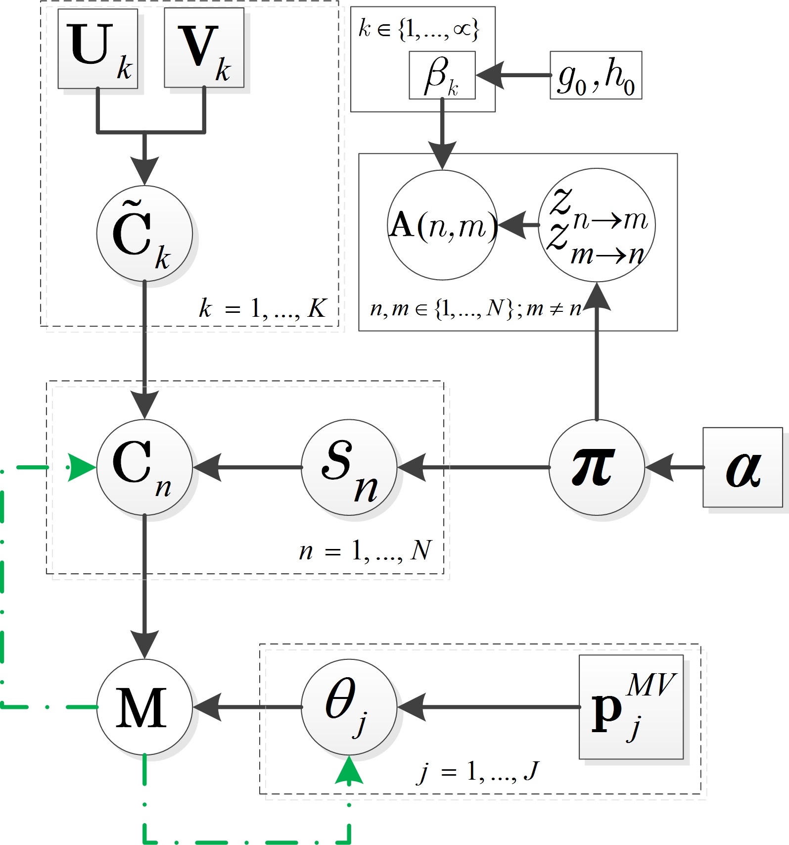
One problem of learning the observation model is that optimizing its neural network weights can become stuck in less attractive local optima [42]. To mitigate this, proper constraints on key latent variables and need to be introduced. In this paper, we use a Bayesian network model (see Fig. 1) to construct interpretable constraints. The Bayesian network model not only guides the learning process but also enables to use the community information of the social network linking the agents together. We explain each component of our Bayesian network model below.
II-B1 Community reliability matrix
We assume that a social network connecting the agents is known. Agents in a social network tend to form communities [46], where a community consists of agents with similar opinion. The community that an agent belongs to is stochastic and unknown a priori but the maximum possible number of communities in the network is known to be . We can thus assign an index in an arbitrary fashion to each community. Let be the community index of agent . We discuss the probability model governing below. Here, we describe how depends on . For each , let be a matrix of the same size as representing the reliability of community . We assume
| (2) |
for , where is a hyperparameter. Then can be regarded as a perturbed version of since for . We assume that for , and ,
| (3) |
where and are hyper parameters. Here we use the normal distribution as the prior as it is an effective prior in many real applications and it allows us to simplify the subsequent inference equations. From Fig. 2, we see that are learned from different inputs of the reliability encoder. Different from a traditional autoencoder [47, 48], are not independent and their relationship is modeled by the Bayesian network in Fig. 1. The Bayesian network model guides the learning process of the autoencoder.
II-B2 Community index
We model the community index of agent as
| (4) |
where the mixture weights
| (5) |
with being a concentration hyperparameter and is the Dirichlet distribution. Here we use the Dirichlet distribution since the support of a Dirichlet distribution can be regarded as the probabilities of categorical events. Besides, the Dirichlet distribution is the conjugate prior distribution of the categorical distribution in Eq. 4 and Eq. 6, which thus allows us to derive analytically the posterior distribution of . We use the mixed membership stochastic block model (MMSB)[43] to model the social connection between agents and . In this model, is the community whose belief agent subscribes to due to the social influence from agent . Under the influence of different agents, agent may subscribe to the beliefs of different communities. If both agents and subscribe to the belief of the same community, they are more likely to be connected in the social network. We assume the following:
| (6) |
where is the beta distribution with parameters , , and
| (7) |
with being a small constant. In Eq. 6, we use beta distribution since the beta distribution is a conjugate prior for the Bernoulli distribution in Eq. 7. Note that is independent of when is given, as shown in Fig. 1.
II-B3 Event states
A direct method to perform truth discovery is majority voting, i.e., selecting the opinion expressed by the most number of agents as the true state of the event. This assumes that all agents have the same reliability, and that agents are more likely to give the correct opinion than not. Without any prior information, this is a reasonable assumption. Therefore, we let the prior of to be given by
| (8) |
for each , where for is the proportion of agents who thinks that the state of event is . We assume that are independent.
III ART: Autoencoder Truth Discovery
In this section, we propose an autoencoder based on unsupervised variational inference [49] for the Bayesian model in Fig. 1.
Let , , , , , and . For simplicity, let . As the closed-form of the posterior distribution is not available, the variational inference method uses a proposal or variational distribution to approximate the posterior distribution, where the parameters in the vector are called the variational parameters. Note that and are assumed to be observed throughout and not included explicitly in our notation for . More specifically, the variational parameters are selected to minimize the following cost function:
| (9) |
where the expectation is over the random variable with distribution conditioned on and . To simplify the optimization procedure, we use the mean-field assumption that is widely used in the literature[50, 49] by choosing
| (10) |
where , , , , , , and are the variational parameters.
In the sequel, to simplify notations, we omit the variational parameters in our notations, e.g., we write instead of . We let . From the graphical model in Fig. 1, we obtain
| (11) |
where is the conditional distribution of the output of the decoder network in Fig. 2. We have made its dependence on the decoder network parameters explicit.
To find the variational parameters, we perform an iterative optimization of in which the optimal parameter solutions are updated iteratively at each step. We substitute (10) and (11) into (9) to obtain
| (12) |
where the constant term does not contain any variational parameters, and {dgroup*}
| (13) |
| (14) |
We update , by minimizing and update , , by minimizing . Furthermore, we update and by minimizing {dgroup*}
| (15) |
| (16) |
Equations (15) and (16) show and can be updated by minimizing
and
respectively.
The variational parameters are optimized and the variational distributions updated iteratively in a procedure that we call AutoencodeR Truth (ART) discovery (since we make use of an autoencoder network described below). Its high-level pseudo code for the -th iteration is shown in Algorithm 1. In the following, we describe how the variational distributions are chosen and how the estimate for the optimal variational parameters are updated in each iteration.
III-A Reliability and Event Encoders
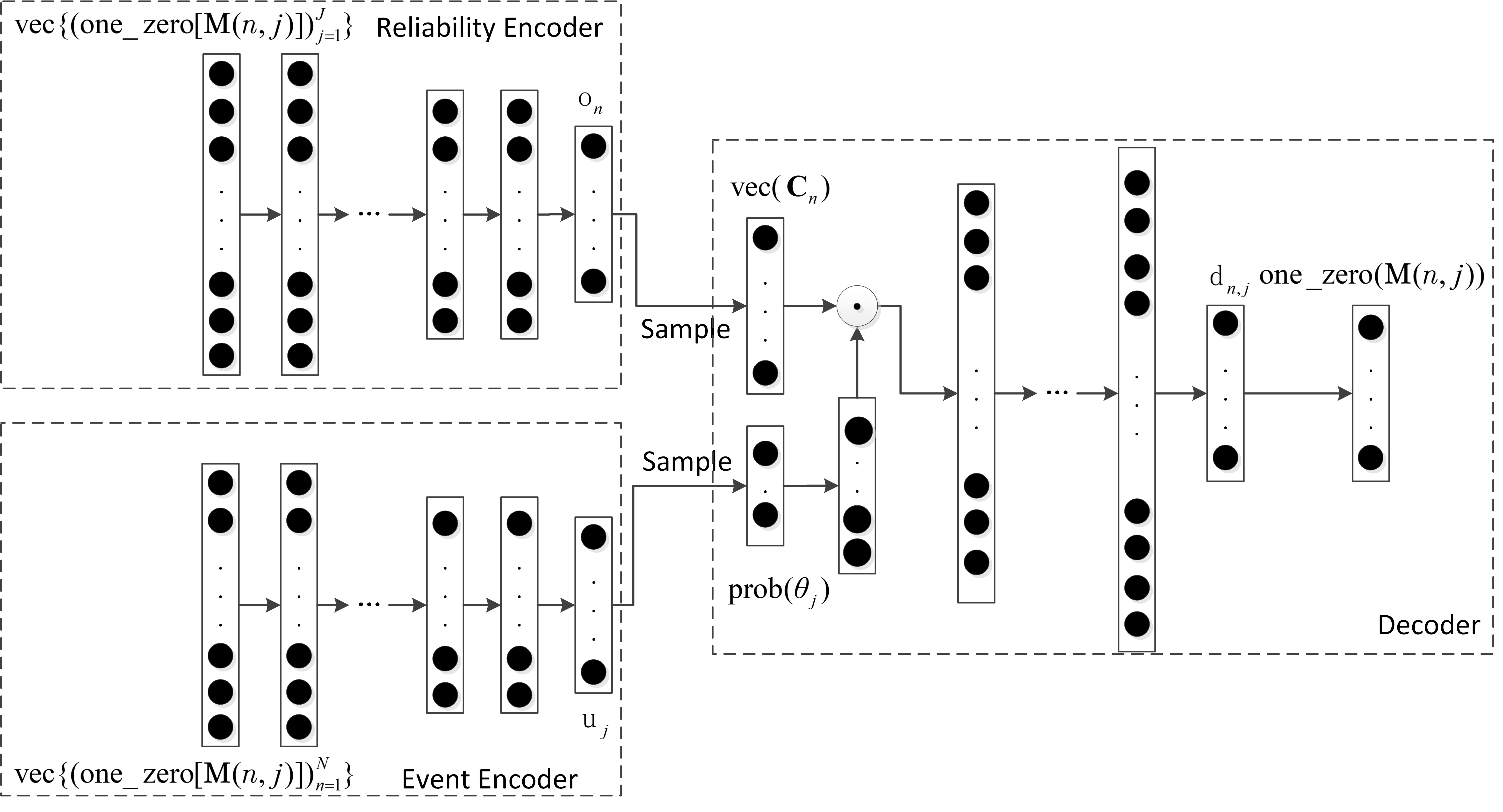
We model and as two encoder networks with parameters and , respectively. These two encoders form part of the autoencoder shown in Fig. 2 with the observation model for given in Section II-A as the decoder network. The details of the two encoder networks are as follows.
- 1.
The reliability encoder network is used to infer the reliability of each agent , with as its input. If is null, then is a zero vector. All the layers of this encoder are fully connected. Let its parameters be and its softmax output be . We assume
(17) where is a hyperparameter.
- 2.
The event encoder network is used to infer the state of each event from . All the layers are also fully connected. Let its parameters be and its output be . We assume
(18)
III-B Updating of
The relationship between and is complex and nonlinear. As discussed before in Sections II-A and III-A, we use neural networks to model and we aim to optimize these neural networks to minimize . From (13), we have {dgroup*}
| (19) |
Recall that , and denote the parameters of the decoder network, the reliability encoder network and the event encoder network, respectively. To learn with the gradient descent method, we need to compute the gradient of with respect to . Denoting the two expectation terms of (19) as and , namely
| (20) |
and we have
As is a discrete variable, is easy to compute. The gradient of with respect to is given by {dgroup*}
which can be computed using the stochastic gradient descent (SGD) algorithm. In each iteration, we replace with its unbiased estimator , where
| (21) |
with , , , and being sampled from , , , and respectively.
We cannot use the same process to deal with and . This is because
as is the parameter of . The same reason applies for . To obtain unbiased estimators for these variational parameters, we need to use the reparameterization trick [51].
From (17), we have , where is generated by the reliability encoder network and is a hyperparameter. We can reparameterize as
| (22) |
From (18), , where the weight vector is generated by the event encoder network. Then, according to (1) in [52], we can reparameterize as
| (23) |
where the Gumbel(0, 1) distribution can be sampled by first drawing and then computing . With and being (22) and (23) respectively, and letting , and , we then obtain
where is the Gaussian probability density function with mean and variance . Here, is a function of and is a function of . We also have
| (24) |
Now in each iteration, we can apply SGD to find an unbiased estimator of the gradient of with respect to and .
Remark 1.
Remark 2.
The term in Eq. 20 is used to constrain the distance between the variational distribution and the prior distribution of event states. When the dataset includes enough observations or useful social network information, then is more important in the initial iterations and the importance decreases as the number of iterations increases. In these cases, we revise Eq. 20 to
| (26) |
where is a hyperparameter and denotes the -th iteration.
III-C Updating of
We want to find variational parameters corresponding to to minimize . To achieve this, we iteratively update these variational parameters in ART. The variational parameters corresponding to and are updated in the same way as our previous work [34]. For completeness, we reproduce the results below.
III-C1 Social network parameter
Let . We choose the variational distribution of to be in the same exponential family as its posterior distribution, namely . Similar to (14) and (15) in our previous work[34], we can show that
| (27) | ||||
| (28) |
where is defined in Section III-C2.
From (10) in [53], we also have
| (29) | ||||
| (30) |
which are used in computing the variational distributions of other parameters in our model. Here, is the digamma function.
III-C2 Community membership indicators
We let the variational distribution of to be in the same exponential family as its posterior distribution, namely a categorical distribution with probabilities . Similar to (19) in our previous work[34], one can show that if ,
| (31) |
where and are computed using (29) and (45) in the sequel, respectively. On the other hand, if , we have
| (32) |
where is computed in (30) in the sequel.
III-C3 Event community indices
We take , where is the variational parameter. Let . We have
Thus, is a categorical distribution and is in the same exponential family as . Let
The natural parameter of is
| (33) |
Assume the natural parameter of is
| (34) |
where . Acording to the relationship between the natural gradient and and the natural parameters (i.e., (22) in [49]), the natural gradient of in (15) with respect to can be derived from (33) and (34) and the result is
We sample from and obtain the unbiased estimator of as
| (35) |
where and it is constant for . Then we update using
| (36) |
where is the known step size at -th iteration. Let be the first three terms of the right-hand side of (35). We compute exponential function of both sides of (36) and obtain
| (37) |
where and are variational parameters of defined in Section III-C4 and can be computed by (45) below. Since and is constant for every , , in each iteration, we only need to compute and then
| (38) |
III-C4 Community reliability matrix
We let the variational distribution of for each to be given by
| (39) |
We also have
| (40) |
which is a normal distribution with mean (cf. Eqs. 2 and 3)
and variance
Let and . As is in the same exponential family as and its natural parameter is . Similar to Section III-C3, we sample from and update and using {dgroup}
| (41) |
| (42) |
Finally, we obtain
III-C5 Mixture weights
We let and thus is an exponential family distribution and its variational parameter is also its natural parameter. To find the variational parameter that minimizes , we find the partial derivative
| (43) |
where
Recall that represents the maximum number of communities. As is in the same exponential family as , thus if we let (43) be zero, we obtain
| (44) |
From (10) in [53], we also have
| (45) |
which is used in (38). Recall that is the digamma function.
IV Experimental Results
In this section, experiments on three real datasets are presented11 1 Code: https://github.com/yitianhoulai/ART. We adopt majority voting, BCC [27], CBCC [29], VISIT [34], TruthFinder[19], AccuSim[20], GTM[54], CRH[55], CATD[21], and KDEm [26] as the state-of-the-art benchmark methods. We test the performance of different methods on the IMDB dataset augmented with Twitter information, which we have made available in [56]. We also test the performance of different methods on the Sentiment Polarity (SP) dataset and the Weather Sentiment (CF) dataset. The last two datasets do not provide network information. To emulate network information in our experiments, for any pair of agents, we calculate the observation differences of their commonly observed events. Next, we calculate the mean of the absolute values of the differences and assume the pair of agents are connected if the mean is less than or equal to 0.2.
IV-A Description of Datasets
IV-A1 Sentiment Polarity (SP) Dataset
The Sentiment Polarity dataset [57] contains agent classifications for movie comments. All the movie comments are from the website Rotten Tomatoes.22 2 https://www.rottentomatoes.com/ Agents were asked to annotate each comment as either positive (1) or negative (0). The uncertainty or confidence of the agents’ annotations are however unavailable. Ground truth labels are from experts. The dataset contains 27,746 evaluations from 203 agents on 4,999 movie comments (i.e., events).
IV-A2 IMDB Dataset
We collected data from the website IMDB33 3 https://www.imdb.com/ and Twitter [56]. If a user rates a movie in IMDB and clicks the share button, a Twitter message is generated. We collected movie evaluations from IMDB and social network information from Twitter. We divide the movie evaluations into 2 levels: bad (0-5), good(6-10). We treat the ratings on the IMDB website, which are based on the aggregated evaluations from all users, as the event truths whereas our observations come from only a subset of users who share their ratings on Twitter. To better show the influence of social network information on event truth discovery, we delete small subnetworks that have less than 5 agents each. The final dataset [56] we use consists of 2266 evaluations from 209 individuals on 245 movies (events) and also the social network between these 209 individuals. Similar to [58, 59], we regard the social network to be undirected as both follower or following relationships indicate that the two users have similar taste.
IV-A3 Weather Sentiment (CF) Dataset
The Weather Sentiment dataset was provided by Crowd-Flower (CF) and can be found in [57]. The agents were asked to classify the tweets with respect to the weather sentiment into the following categories: negative (0), neutral (1), positive (2), tweet not related to weather (3) and cannot tell (4). The dataset contains 1,720 evaluations from 461 agents on 300 tweets (i.e., events).
IV-B Experiment Settings
The hyperparameters in our proposed ART method are tuned using another dataset called MS from [57]. Since the hyperparameters of our method are tuned with this dataset, we do not compare the performance of ART and the benchmark methods on this dataset. The values of the hyperparameters in our method are given in Table II. We use the same set of hyperparameters except to do experiments on all the three datasets in Section IV-A.
| Hyper-parameter | Value |
|---|---|
| in (7) | |
| in (17) and in (2) | 0.1 |
| Each element of in (3) | Random value between 0.4 and 0.5 |
| Each element of in (3) | |
| in (25) | 0.01 |
| Maximum number of communities | 3 |
| Size of the reliability matrices | 63 |
| Sizes of 2 hidden layers of the reliability encoder | 128, and 32 |
| Sizes of 2 hidden layers of the event encoder | 128, and 32 |
| Sizes of 3 hidden layers of the decoder | 16, 32, and 128 |
| Learning rate of ADAMS optimizer | 0.001 |
| Step size at -th iteration | |
| in Eq. 26 | IMDB and SP: 0.9; CF:1.0 |
IV-C Sensitivity Analysis
We conduct experiments on the three datasets using the same set of hyperparameters except in Eq. 26. The CF dataset contains only 1,720 observations and has no social network information and thus the majority voting prior is important in all the learning iterations. We thus set be 1.0. For the IMDB and SP datasets, we set to be 0.9 since the SP dataset is rich in observations and the IMDB dataset contains social network information. For these two datasets, the importance of the majority voting prior decreases as the iteration progresses. The results in Section IV-D suggest that our method is not sensitive to the hyperparameters and can achieve the comparable accuracies on different datasets using the same set of hyperparameters except . In the following, we perform experiments to show the influence of different hyperparameters on our method.
IV-C1 Impact of reliability matrice size
ART uses reliability matrices to represent the reliabilities of agents. In this experiment, we study impact of 4 different reliability matrix sizes on the truth discovery accuracy. The results show that the accuracy of ART is related to the number of elements (i.e., the product of and ) in the reliability matrices. We observe that reliability matrices of size and achieve the same accuracies on all three real datasets. However, we also observe that different sizes of the matrix all achieve comparable results.
| SP | IMDB | CF | |
|---|---|---|---|
| 2 9 | 0.918 | 0.771 | 0.903 |
| 6 3 | 0.918 | 0.771 | 0.903 |
| 3 3 | 0.914 | 0.767 | 0.890 |
| 6 6 | 0.915 | 0.763 | 0.897 |
IV-C2 Impact of number of communities
In this experiment, we show the impact of the number of communities on the truth discovery accuracy of ART. From Table IV, we observe that ART achieves relatively good accuracies on all three datasets with different number of communities.
| SP | IMDB | CF | |
|---|---|---|---|
| 3 | 0.918 | 0.771 | 0.903 |
| 6 | 0.915 | 0.759 | 0.9 |
| 9 | 0.915 | 0.788 | 0.89 |
IV-C3 Impact of variance
In ART, we use to denote the variance of the prior distribution of . From Table V, we observe that different have larger influence on CF than the other two datasets. ART achieves the best accuracies on all the three datasets when each element of is 0.1.
| Each element of | SP | IMDB | CF |
|---|---|---|---|
| 0.01 | 0.916 | 0.771 | 0.867 |
| 0.1 | 0.918 | 0.771 | 0.903 |
| 1 | 0.917 | 0.771 | 0.877 |
IV-D Comparison with Benchmarks
We evaluate and compare the performance of ART and the benchmark methods using five metrics: accuracy, area under the ROC curve (AUC), precision, recall, and the F1 score. The top performer and those close to it (i.e, within 0.002 of the top) are highlighted in boldface in the subsequent tables. The following results indicate that ART is competitive, and often superior, compared to the other benchmark methods. However, the computation time of ART is larger than most of the other benchmark methods (except VISIT) since we include the agent network information in our inference. Our deep autoencoder is also more computationally expensive to learn.
IV-D1 Accuracy
The accuracies of ART and the benchmark methods are shown in Table VI. It can be observed that ART achieves the best accuracies on all the three datasets.
| Method | SP | IMDB | CF |
|---|---|---|---|
| ART | 0.918 | 0.771 | 0.903 |
| VISIT | 0.916 | 0.751 | 0.893 |
| CBCC | 0.916 | 0.714 | 0.893 |
| BCC | 0.915 | 0.678 | 0.890 |
| MV | 0.885 | 0.710 | 0.867 |
| TruthFinder | 0.885 | 0.714 | 0.880 |
| AccuSim | 0.890 | 0.702 | 0.730 |
| GTM | 0.890 | 0.710 | 0.743 |
| CRH | 0.894 | 0.706 | 0.747 |
| CATD | 0.873 | 0.657 | 0.807 |
| KDEm | 0.890 | 0.702 | 0.877 |
IV-D2 Area under the ROC Curve (AUC)
The AUC scores of ART and the benchmark methods are shown in Table VII. For the multi-class case (i.e., the CF dataset), AUC scores are calculated for each label, and their average is taken. It can be observed that ART achieves the best AUC score on the SP dataset and is among one of the best methods on the CF dataset. On the IMDB dataset, VISIT and BCC achieve the best AUC scores.
| Method | SP | IMDB | CF |
|---|---|---|---|
| ART | 0.958 | 0.844 | 0.948 |
| VISIT | 0.958 | 0.871 | 0.913 |
| CBCC | 0.957 | 0.859 | 0.949 |
| BCC | 0.957 | 0.872 | 0.950 |
| MV | 0.885 | 0.759 | 0.865 |
| TruthFinder | 0.885 | 0.765 | 0.873 |
| AccuSim | 0.890 | 0.753 | 0.754 |
| GTM | 0.890 | 0.759 | 0.763 |
| CRH | 0.894 | 0.756 | 0.764 |
| CATD | 0.873 | 0.708 | 0.824 |
| KDEm | 0.890 | 0.753 | 0.861 |
IV-D3 Precision
The precision scores of ART and the benchmark methods are shown in Table VIII. For the multi-class case (i.e., the CF dataset), precisions are calculated for each label, and their average, weighted by the number of true instances for each label, is taken. It can be observed that ART achieves the best precision on the IMDB dataset and is one of the best methods on the SP dataset. On the CF dataset, CBCC achieves the best precision.
| Method | SP | IMDB | CF |
|---|---|---|---|
| ART | 0.921 | 0.639 | 0.878 |
| VISIT | 0.922 | 0.607 | 0.896 |
| CBCC | 0.922 | 0.568 | 0.902 |
| BCC | 0.92 | 0.535 | 0.865 |
| MV | 0.868 | 0.563 | 0.873 |
| TruthFinder | 0.868 | 0.566 | 0.885 |
| AccuSim | 0.886 | 0.556 | 0.748 |
| GTM | 0.874 | 0.563 | 0.762 |
| CRH | 0.884 | 0.559 | 0.758 |
| CATD | 0.863 | 0.519 | 0.824 |
| KDEm | 0.878 | 0.556 | 0.879 |
IV-D4 Recall
The recall scores of ART and the benchmark methods are shown in Table IX. For the multi-class case (i.e., the CF dataset), recall scores are calculated for each label, and then their average, weighted by the number of true instances for each label, is taken. It can be observed that ART achieves the best recall on two datasets: the SP and CF datasets. On the IMDB dataset, TruthFinder achieves the best recall.
| Method | SP | IMDB | CF |
|---|---|---|---|
| ART | 0.913 | 0.867 | 0.903 |
| VISIT | 0.910 | 0.911 | 0.893 |
| CBCC | 0.910 | 0.933 | 0.893 |
| BCC | 0.909 | 0.944 | 0.890 |
| MV | 0.907 | 0.944 | 0.867 |
| TruthFinder | 0.907 | 0.956 | 0.880 |
| AccuSim | 0.894 | 0.944 | 0.730 |
| GTM | 0.911 | 0.944 | 0.743 |
| CRH | 0.907 | 0.944 | 0.747 |
| CATD | 0.887 | 0.900 | 0.807 |
| KDEm | 0.906 | 0.944 | 0.877 |
IV-D5 F1 score
The F1 scores of ART and the benchmark methods are shown in Table X. For the multi-class case (i.e., the CF dataset), F1 scores are calculated for each label, and their average, weighted by the number of true instances for each label, is taken. This averaging takes label imbalance into consideration and can result in an F1 score that is not between the corresponding precision and recall. It can be observed that ART achieves the best F1 scores on two datasets: the IMDB and SP datasets. On the CF dataset, ART is slightly worse than VISIT, which achieves the best F1 score.
| Method | SP | IMDB | CF |
|---|---|---|---|
| ART | 0.917 | 0.736 | 0.890 |
| VISIT | 0.916 | 0.729 | 0.894 |
| CBCC | 0.916 | 0.706 | 0.884 |
| BCC | 0.914 | 0.683 | 0.877 |
| MV | 0.887 | 0.705 | 0.868 |
| TruthFinder | 0.887 | 0.711 | 0.882 |
| AccuSim | 0.890 | 0.700 | 0.712 |
| GTM | 0.892 | 0.705 | 0.731 |
| CRH | 0.895 | 0.702 | 0.730 |
| CATD | 0.875 | 0.659 | 0.814 |
| KDEm | 0.891 | 0.700 | 0.876 |
IV-D6 Average execution time
We tabulate the average execution time of ART and the benchmark methods in Table XI. All the methods are run on the same laptop with a core-i5-8250U CPU and 16G RAM.
The execution time of ART is over 100 times larger than most of the benchmark methods since ART includes the agent network information and the deep autoencoder is computationally expensive to learn. The SP dataset contains the largest number of evaluations and the CF dataset contains the largest number of agents and thus experiments on these two datasets take more time. Another benchmark that uses the agent network information is VISIT, which however has longer average execution times than ART due to the complex variational inference approach used in its non-conjugate observation model. ART is therefore more suitable for offline truth discovery applications, where inference performance is more important than latency.
| Method | SP | IMDB | CF |
|---|---|---|---|
| ART | 1261.1 | 92.0 | 118.8 |
| VISIT | 1413.6 | 108.5 | 562.1 |
| CBCC | 4.0 | 2.4 | 4.2 |
| BCC | 5.1 | 1.7 | 1.9 |
| MV | 1.0 | 0.1 | 0.1 |
| TruthFinder | 0.4 | 0.1 | 0.1 |
| AccuSim | 41.9 | 3.2 | 0.8 |
| GTM | 1.0 | 0.1 | 0.1 |
| CRH | 1.5 | 0.1 | 0.1 |
| CATD | 0.5 | 0.1 | 0.1 |
| KDEm | 0.9 | 0.1 | 0.1 |
V Conclusion
In this paper, we have combined the strength of autoencoders in learning nonlinear relationships and the strength of Bayesian networks in characterizing hidden interpretable structures to tackle the truth discovery problem. The Bayesian network model introduces constraints to the autoencoder and at the same time incorporates the community information of the social network into the autoencoder. We developed a variational inference method to estimate the parameters in the autoencoder and infer the hidden variables in the Bayesian network. Results on real datasets demonstrate the competitiveness of our proposed method over other state-of-the-art benchmark methods.
In this paper, we have not considered correlations between events in our inference. We have also not incorporated any side information or prior information about the events into our procedure. These are interesting future research directions, which may further improve the truth discovery accuracy.
References
- [1] D. R. Karger, S. Oh, and D. Shah, “Efficient crowdsourcing for multi-class labeling,” ACM SIGMETRICS Performance Evaluation Review, vol. 41, no. 1, pp. 81–92, 2013.
- [2] D. Acemoglu, M. A. Dahleh, I. Lobel, and A. Ozdaglar, “Bayesian learning in social networks,” Review of Economic Studies, vol. 78, no. 4, pp. 1201–1236, Mar. 2011.
- [3] J. Ho, W. P. Tay, T. Q. S. Quek, and E. K. P. Chong, “Robust decentralized detection and social learning in tandem networks,” IEEE Trans. Signal Process., vol. 63, no. 19, pp. 5019 – 5032, Oct. 2015.
- [4] W. P. Tay, “Whose opinion to follow in multihypothesis social learning? A large deviations perspective,” IEEE J. Sel. Topics Signal Process., vol. 9, no. 2, pp. 344 – 359, Mar. 2015.
- [5] M. L. Gray, S. Suri, S. S. Ali, and D. Kulkarni, “The crowd is a collaborative network,” in ACM Conf. Computer-Supported Cooperative Work & Social Computing, 2016, pp. 134–147.
- [6] C. Huang and D. Wang, “Topic-aware social sensing with arbitrary source dependency graphs,” in ACM/IEEE Int. Conf. Inform. Process. Sensor Networks, 2016, pp. 1–12.
- [7] Q. Kang and W. P. Tay, “Sequential multi-class labeling in crowdsourcing,” IEEE Trans. Knowl. Data Eng., vol. 31, no. 11, pp. 2190–2199, 2019.
- [8] L. Berti-Equille and J. Borge-Holthoefer, “Veracity of data: From truth discovery computation algorithms to models of misinformation dynamics,” Synthesis Lectures on Data Management, vol. 7, no. 3, pp. 1–155, 2015.
- [9] Y. Li, J. Gao, C. Meng, Q. Li, L. Su, B. Zhao, W. Fan, and J. Han, “A survey on truth discovery,” ACM Sigkdd Explorations Newslett., vol. 17, no. 2, pp. 1–16, 2016.
- [10] P. Cheng, X. Lian, L. Chen, J. Han, and J. Zhao, “Task assignment on multi-skill oriented spatial crowdsourcing,” IEEE Trans. Knowledge and Data Engineering, vol. 28, no. 8, pp. 2201–2215, 2016.
- [11] Y. Tong, L. Chen, Z. Zhou, H. V. Jagadish, L. Shou, and W. Lv, “Slade: A smart large-scale task decomposer in crowdsourcing,” IEEE Trans. Knowl. and Data Eng., vol. 30, no. 8, pp. 1588–1601, 2018.
- [12] T. Tian, Y. Zhou, and J. Zhu, “Selective verification strategy for learning from crowds,” in AAAI Conf. Artificial Intelligence, 2018.
- [13] M. Alsayasneh, S. Amer-Yahia, E. Gaussier, V. Leroy, J. Pilourdault, R. M. Borromeo, M. Toyama, and J. Renders, “Personalized and diverse task composition in crowdsourcing,” IEEE Trans. Knowl. and Data Eng., vol. 30, no. 1, pp. 128–141, 2017.
- [14] Y. Wang, F. Ma, Z. Jin, Y. Yuan, G. Xun, K. Jha, L. Su, and J. Gao, “Eann: Event adversarial neural networks for multi-modal fake news detection,” in Proceedings of the 24th acm sigkdd international conference on knowledge discovery & data mining, 2018, pp. 849–857.
- [15] D. Wang, L. Kaplan, H. Le, and T. Abdelzaher, “On truth discovery in social sensing: A maximum likelihood estimation approach,” in ACM/IEEE Int. Conf. Inform. Process. Sensor Networks, 2012, pp. 233–244.
- [16] B. Zhao, B. I. P. Rubinstein, J. Gemmell, and J. Han, “A Bayesian approach to discovering truth from conflicting sources for data integration,” Proc. VLDB Endowment, vol. 5, no. 6, pp. 550–561, 2012.
- [17] D. Wang, M. T. Amin, S. Li, T. Abdelzaher, L. Kaplan, S. Gu, C. Pan, H. Liu, C. C. Aggarwal, and R. Ganti, “Using humans as sensors: an estimation-theoretic perspective,” in ACM/IEEE Int. Conf. Inform. Process. Sensor Networks, 2014, pp. 35–46.
- [18] S. Yao, S. Hu, S. Li, Y. Zhao, L. Su, L. Kaplan, A. Yener, and T. Abdelzaher, “On source dependency models for reliable social sensing: Algorithms and fundamental error bounds,” in IEEE Int. Conf. Distributed Computing Syst., 2016, pp. 467–476.
- [19] X. Yin, J. Han, and S. Y. Philip, “Truth discovery with multiple conflicting information providers on the web,” IEEE Trans. Knowl. Data Eng., vol. 20, no. 6, pp. 796–808, 2008.
- [20] X. L. Dong, L. Berti-Equille, and D. Srivastava, “Integrating conflicting data: the role of source dependence,” Proc. VLDB Endowment, vol. 2, no. 1, pp. 550–561, 2009.
- [21] Q. Li, Y. Li, J. Gao, L. Su, B. Zhao, M. Demirbas, W. Fan, and J. Han, “A confidence-aware approach for truth discovery on long-tail data,” Proc. VLDB Endowment, vol. 8, no. 4, pp. 425–436, 2015.
- [22] D. Y. Zhang, D. Wang, and Y. Zhang, “Constraint-aware dynamic truth discovery in big data social media sensing,” in IEEE Int. Conf. Big Data, 2017, pp. 57–66.
- [23] X. Zhang, Y. Wu, L. Huang, H. Ji, and G. Cao, “Expertise-aware truth analysis and task allocation in mobile crowdsourcing,” in IEEE Int. Conf. Distributed Computing Syst., 2017, pp. 922–932.
- [24] Y. Li, B. I. P. Rubinstein, and T. Cohn, “Truth inference at scale: A Bayesian model for adjudicating highly redundant crowd annotations,” in Int. Conf. World Wide Web, 2019.
- [25] K. Broelemann, T. Gottron, and G. Kasneci, “Ltd-rbm: Robust and fast latent truth discovery using restricted boltzmann machines,” in 2017 IEEE 33rd International Conference on Data Engineering (ICDE), 2017, pp. 143–146.
- [26] M. Wan, X. Chen, L. Kaplan, J. Han, J. Gao, and B. Zhao, “From truth discovery to trustworthy opinion discovery: An uncertainty-aware quantitative modeling approach,” in Proceedings of the 22nd ACM SIGKDD International Conference on Knowledge Discovery and Data Mining, 2016, pp. 1885–1894.
- [27] H. C. Kim and Z. Ghahramani, “Bayesian classifier combination,” in Artificial Intell. and Stat., 2012, pp. 619–627.
- [28] Y. Zheng, G. Li, Y. Li, C. Shan, and R. Cheng, “Truth inference in crowdsourcing: is the problem solved?” Proc. VLDB Endowment, vol. 10, no. 5, pp. 541–552, 2017.
- [29] M. Venanzi, J. Guiver, G. Kazai, P. Kohli, and M. Shokouhi, “Community-based Bayesian aggregation models for crowdsourcing,” in Int. Conf. World Wide Web, 2014, pp. 155–164.
- [30] S. Lyu, W. Ouyang, Y. Wang, H. Shen, and X. Cheng, “Truth discovery by claim and source embedding,” IEEE Trans. Knowl. Data Eng., 2019.
- [31] Y. Li, B. Rubinstein, and T. Cohn, “Exploiting worker correlation for label aggregation in crowdsourcing,” in Int. Conf. Machine Learning, 2019, pp. 3886–3895.
- [32] M. Yin, M. L. Gray, S. Suri, and J. W. Vaughan, “The communication network within the crowd,” in Int. Conf. World Wide Web, 2016, pp. 1293–1303.
- [33] L. Ma, W. P. Tay, and G. Xiao, “Iterative expectation maximization for reliable social sensing with information flows,” Information Sciences, 2018, accepted.
- [34] J. Yang, J. Wang, and W. P. Tay, “Using social network information in community-based Bayesian truth discovery,” IEEE Trans. Signal Inf. Process. Netw., 2019, accepted.
- [35] A. Krizhevsky, I. Sutskever., and G. E. Hinton, “Imagenet classification with deep convolutional neural networks,” in Advances in Neural Information Processing Systems, 2012, pp. 1097–1105.
- [36] J. L. Elman, “Finding structure in time,” COGNITIVE SCIENCE, vol. 14, no. 2, pp. 179–211, 1990.
- [37] J. Marshall, A. Argueta, and D. Wang, “A neural network approach for truth discovery in social sensing,” in 2017 IEEE 14th international conference on mobile Ad Hoc and sensor systems (MASS). IEEE, 2017, pp. 343–347.
- [38] L. Li, B. Qin, W. Ren, and T. Liu, “Truth discovery with memory network,” Tsinghua Science and Technology, vol. 22, no. 6, pp. 609–618, 2017.
- [39] M. Johnson, D. K. Duvenaud, A. Wiltschko, R. P. Adams, and S. R. Datta, “Composing graphical models with neural networks for structured representations and fast inference,” in Advances in neural information processing systems, 2016, pp. 2946–2954.
- [40] M. Dundar, B. Krishnapuram, J. Bi, and R. B. Rao, “Learning classifiers when the training data is not iid.” in Int. Joint Conf. Artificial Intell., 2007, pp. 756–761.
- [41] D. P. Kingma and M. Welling, “Auto-encoding variational bayes,” arXiv preprint arXiv:1312.6114, 2013.
- [42] B. Zong, Q. Song, M. R. Min, W. Cheng, C. Lumezanu, D. Cho, and H. Chen, “Deep autoencoding gaussian mixture model for unsupervised anomaly detection,” in Int. Conf. Learning Representations, 2018.
- [43] E. M. Airoldi, D. M. Blei, S. E. Fienberg, and E. P. Xing, “Mixed membership stochastic blockmodels,” J. Mach. Learning Research, vol. 9, no. Sep, pp. 1981–2014, 2008.
- [44] Y. W. Teh, M. I. Jordan, M. J. Beal, and D. M. Blei, “Hierarchical Dirichlet processes,” J. Am. Stat. Assoc., 2012.
- [45] D. M. Blei, A. Y. Ng, and M. I. Jordan, “Latent dirichlet allocation,” J. machine Learning research, vol. 3, no. Jan, pp. 993–1022, 2003.
- [46] S. Fortunato and D. Hric, “Community detection in networks: A user guide,” Physics Rep., vol. 659, pp. 1–44, 2016.
- [47] Y. Bengio, L. Yao, G. Alain, and P. Vincent, “Generalized denoising auto-encoders as generative models,” in Advances in Neural Information Processing Systems, 2013, pp. 899–907.
- [48] I. Goodfellow, Y. Bengio, and A. Courville, Deep Learning. MIT Press, 2016, http://www.deeplearningbook.org.
- [49] M. D. Hoffman, D. M. Blei, C. Wang, and J. Paisley, “Stochastic variational inference,” J. Mach. Learning Research, vol. 14, no. 1, pp. 1303–1347, 2013.
- [50] D. M. Blei and M. I. Jordan, “Variational inference for dirichlet process mixtures,” Bayesian analysis, vol. 1, no. 1, pp. 121–143, 2006.
- [51] D. P. Kingma, “Variational inference & deep learning: A new synthesis,” Ph.D. dissertation, University of Amsterdam, 2017.
- [52] E. Jang, S. Gu, and B. Poole, “Categorical reparameterization with Gumbel-softmax,” arXiv preprint arXiv:1611.01144, 2016.
- [53] T. Minka, Bayesian inference, entropy, and the multinomial distribution, 2003. [Online]. Available: https://tminka.github.io/papers/minka-multinomial.pdf
- [54] B. Zhao and J. Han, “A probabilistic model for estimating real-valued truth from conflicting sources,” Proc. of QDB, 2012.
- [55] Q. Li, Y. Li, J. Gao, B. Zhao, W. Fan, and J. Han, “Resolving conflicts in heterogeneous data by truth discovery and source reliability estimation,” in Proc. ACM SIGMOD int. conf. Management of data, 2014, pp. 1187–1198.
- [56] J. Yang and W. P. Tay. (2018) Using social network information to discover truth of movie ranking. [Online]. Available: https://doi.org/10.21979/N9/L5TTRW
- [57] M. Venanzi, O. Parson, A. Rogers, and N. Jennings, “The ActiveCrowdToolkit: An open-source tool for benchmarking ActiveLearning algorithms for crowdsourcing research,” in 3rd Human Computation and Crowdsourcing Conference (HCOMP), 2015. [Online]. Available: https://github.com/orchidproject/active-crowd-toolkit/tree/master/Data
- [58] S. Fortunato, “Community detection in graphs,” Physics Rep., vol. 486, no. 3, pp. 75–174, 2010.
- [59] P. K. Gopalan and D. M. Blei, “Efficient discovery of overlapping communities in massive networks,” Proc. Nat. Academy Sci., vol. 110, no. 36, pp. 14 534–14 539, 2013.