Joint State Estimation Under Attack of Discrete Event Systems

The problem of estimation under attack has been considered by relatively few authors in the automatic control literature.

In [30, 31, 32] the state estimation problem for time-driven models is studied.

Ding et al. [30] propose the problem of remote state estimation under denial-of-service attacks. A sensor needs to choose a channel to transmit the data packets, while an attacker needs to choose a channel to attack. They formalize such a problem as a two player stochastic game between the sensor and the attacker, and present optimal strategies in terms of computational complexity for both sides, respectively.

Peng et al. [31] consider the issue of optimal attack energy allocation against remote state estimation. An optimal attack strategy that can result in maximal estimation error covariances is derived. Finally, they prove that the optimal strategy has a threshold structure.

Cheng et al. [32] develop an attack strategy that can degrade the estimation performance by tampering with the sensors, eavesdropping the measurements, and injecting false feedback information. They conclude that, with the presence of an attacker, the mean-squared stability condition of the state estimation is weakened.

In this work we consider discrete-event models, and the approaches developed in the above mentioned literature cannot be adopted. The state estimation problem for discrete event systems so far has not been studied in all generality, but has been partially addressed in the context of supervisory control. Here we mention a few recent publications which have inspired our work.

Tong et al. [25] present a new finite structure called parallel observer, which allows to simultaneously describe the observations of the supervisor and of the attacker. Based on the parallel observer, a maximally permissive supervisor is developed to enforce current-state opacity.

Meira-Góes et al. [26] propose a novel bipartite transition structure in the framework of discrete event systems, namely, Insertion-Deletion Attack structure, and present a game-like relationship between the supervisor and the environment (the plant and the attacker) to determine if the attacker can lead the plant to a forbidden state without being detected by the supervisor.

Lima et al. [27] propose a defense policy that prevents cyber attacks at sensor and actuator layer in supervisory control systems. It is assumed that the attacker can alter the observation of events in a set of events $\Sigma_{vs}$, and modify the enabling of events in a set of events $\Sigma_{va}$. The detectable network attack security and undetectable network attack security are introduced to prevent the plant from reaching forbidden states.

Su [28] addresses the problem of attack-with-bounded-sensor-reading-alteration (ABSRA), where the attacker can intercept the sensor readings from the plant and arbitrarily alter them but with an upper bound on the length of the altered observation word. In this way the attacker can cheat the supervisor, which will lead the plant to the undesirable states. The author also develops a supervisor that is robust to ABSRA.

We point out that significant differences exist between the problem setting considered in this paper and the problem setting dealt in most of the papers in the literature, including the above mentioned ones. What we propose is a methodology for studying how the possible choices of the attacker can affect the estimate of the operator. On the contrary, previous works on cyber attacks in the DES literature, including [15, 26, 27, 28], consider the case of an operator/supervisor: in such a case the goal of the attacker is to beguile the supervisor so that a specification is violated, i.e., the plant reaches a forbidden state or generates a forbidden evolution.

The proposed approach can be applied not only to the case in which an operator-supervisor controls a plant in closed-loop — as in the above mentioned papers — but in more general settings, where the operator may have goals of different nature. As an example, in our framework one may study how cyber attacks disturb an operator-monitor which takes decisions based on its estimation of the plant state or an operator-diagnoser which aims to detect the occurrence of faults. Mutatis mutandis, our approach can also be used for addressing a problem of opacity enforcing: in such a case the operator is an intruder that wants to infer a secret and the attacker is the agent that corrupts the observation to thwart the intruder.

This paper contains several original contributions.

• •

  The problem of joint state estimation under attack is formalized; harmful attacks are characterized in general terms by means of a misleading relation.

• •

  Based on the notion of attack alphabet and attack words, which describe how observations can be corrupted by the attacker we show how to construct two different observers: they describe the state estimates computed by the attacker and by the operator for each corrupted observation.

• •

  A formal methodology to design a joint estimator is presented. This automaton, constructed as the concurrent composition of the two observers, describes all possible attacks.

• •

  The joint estimator shows, for each possible corrupted observation, the joint state estimation, i.e., the set of states consistent with the uncorrupted observation and the set of states consistent with the corrupted observation. Such a structure also indicates if a harmful attack exists.

The rest of the paper is organized as follows. In Section II, we recall the basic notions of finite-state automata and of state estimation via observers. In Section III, we first describe the adopted attack model, and then formalize the problem considered in this paper. In Section IV, we develop two observers: attacker observer and operator observer. In Section V, we define the unbounded joint estimator as the concurrent composition of such observers. Then, we define an automaton that allows us, again via concurrent composition, to define a bounded joint estimator, starting from the unbounded one. Conclusions are finally drawn in Section VI where we also discuss our future lines of research in this framework.

In this paper we consider a plant modeled by a partially observable DFA with set of observable events $E_{o}$ and set of unobservable events $E_{uo}$. Referring to Fig. 1, if $\sigma$ is a word generated by the plant, the observed word is $s=P(\sigma)$. An attacker may corrupt the output signals produced by the plant with the effect of inserting in the observation some events that did not occur, or erasing some events that have occurred. Such a corrupted observation is denoted as $s^{\prime}$ (a sequence of events in $E_{o}$), and the operator constructs its state estimation based on $s^{\prime}$. In our framework, we assume the operator monitors the plant to estimate its current state: the objective of the attacker is to corrupt the observation in such a way that a correct estimation is not possible.

The definition of compromised events was first proposed in [26]. However, while in [26] the authors assume that all the compromised events can be inserted and erased by the attacker, here we slightly generalize the definition as follows.

The set of compromised events that can be inserted in the observer evolution is denoted as $E_{ins}$, and the set of events that can be erased is denoted as $E_{era}$. To keep the presentation general, we assume that $E_{ins}$ and $E_{era}$ are not necessarily disjoint.

The relationship among the different subsets of observable events $E_{o}$ is clarified in Fig. 2.

We now formally describe the action of the attacker in terms of two new types of events that it can generate. More precisely, even if it is possible to directly define the attacker as a finite-state transducer that “translates” an observed word $s$ into a corrupted observation $s^{\prime}$ (see Fig. 1), for a reason that will appear clear in the following, we prefer to characterize the attacker’s action in terms of a new word defined on a so-called attack alphabet $E_{a}$.

The set of inserted events [26] is denoted as ${E_{+}}$, namely $E_{+}=\{e_{+}\mid e\in E_{ins}\}$. The occurrence of an event $e_{+}\in E_{+}$ denotes the fact that the attacker inserts in the operator observation an event $e\in E_{ins}$ that has not occurred in reality.

The set of erased events [26] is denoted as ${E_{-}}$, namely $E_{-}=\{e_{-}\mid e\in E_{era}\}$. The occurrence of an event $e_{-}\in E_{-}$ denotes the fact that the attacker erases from the operator’s observation event $e\in E_{era}$ generated by plant.  $\diamond$

Given a bound $n\in\mathbb{N}\cup\{\infty\}$, let $E^{\leq n}_{+}=\{w_{+}\in E^{*}_{+}\ \mid\ |w_{+}|\leq n\}$ denote the set of words on alphabet $E_{+}$ whose length does not exceed $n$. Note that if $n=\infty$ then $E^{\leq n}_{+}=E^{*}_{+}$.

1. (a)

   $f_{n}(\varepsilon)\in E_{+}^{\leq n}$,

2. (b)

   $\forall se\in P(L(G))$ with $s\in E_{o}^{*}$:

   $$\left\{\begin{array}[]{ll}f_{n}(se)\in f_{n}(s)\{e_{-},e\}E_{+}^{\leq n}&\text{if}\quad e\in E_{era},\\ f_{n}(se)\in f_{n}(s)\{e\}E_{+}^{\leq n}&\text{if}\quad e\in E_{o}\setminus E_{era}.\end{array}\right.$$

   (2)

$\diamond$

In Definition 3, condition (a) means that the attacker can insert a bounded word $w_{+}\in E_{+}^{\leq n}$ at the initial state, before any event generated by the plant is observed. Condition (b) implies that if an event $e\in E_{era}$ occurs, the attacker can either erase event $e$ or not erase it, and then insert any word $w_{+}\in E_{+}^{\leq n}$. If an event $e\in E_{o}\backslash E_{era}$ occurs, then the attacker can insert any word $w_{+}\in E_{+}^{\leq n}$ after $e$.

We notice that imposing that the attacker may insert at most $n$ consecutive events between any two observed events, makes sense in practice. Indeed, even if our model is purely logical, a real system can produce in a finite time just a finite number of events. If the attacker could introduce an arbitrarily large number of events between two consecutive observed events, this would lead to an anomalous behavior as observed by the operator.

We denote as ${\mathcal{F}}_{n}$ the set of attack functions for a given $n\in\mathbb{N}\cup\{\infty\}$.

Given two integer numbers $n$ and $n^{\prime}$, ${\mathcal{F}}_{n}\subseteq{\mathcal{F}}_{n^{\prime}}$ if $n\leq n^{\prime}$. Furthermore, ${\mathcal{F}}_{n}\subseteq{\mathcal{F}}_{\infty}$ for all $n<\infty$.

$\diamond$

The internal structure of the attacker is visualized in Fig. 1 as a black box taking an observation $s$ as an input and producing a corrupted observation $s^{\prime}$ as an output. Such an internal structure is sketched in more detail in Fig. 3.

Here the observed word is $s=P(\sigma)$ (a sequence of events in $E_{o}$). The attacker corrupts the observation according to the attack function $f_{n}$, producing $w\in L(f_{n},G)\subseteq E_{a}^{*}$. Such a sequence is projected via $\widehat{P}$ on $E_{o}$, generating a word $s^{\prime}$. The plant operator constructs its state estimation based on $s^{\prime}$.

In this subsection we first describe the possible goals of the attacker on which we are focusing in this paper. Then we formalize the problem statement. To this aim we introduce a relation $\mathcal{R}\subseteq 2^{X}\times 2^{X}$, called a misleading relation. If $s$ and $s^{\prime}$ in $E_{o}^{*}$ denote, respectively, the generic uncorrupted and corrupted observation of the operator, the goal of the attacker is achieved whenever

i.e., whenever the pair (set of states consistent with the uncorrupted observation, set of states consistent with the corrupted observation) belongs to $\mathcal{R}$. The following definition formalizes this.

Different physical problems can be described in this setting by suitably defining relation $\mathcal{R}$. A significant example is the following one.

Given a plant $G=(X,E,\delta,x_{0})$ with set of observable events $E_{o}$, and a misleading relation $\mathcal{R}\subseteq 2^{X}\times 2^{X}$, the main contribution of this paper consists in providing a tool, called a joint estimator that contains all the possible actions (insert and/or erase observations) that an attacker may implement during the system evolution. On the basis of such a structure, the attacker can establish if the attacks are harmful to the plant.

The attacker observer $Obs_{att}(G)$ describes all possible attack words that can be generated by functions in $\mathcal{F}_{\infty}$ and the corresponding sets of consistent states of the system. Since attacks are performed by the attacker, it knows which observations originate from events that have really occurred in the plant ($E_{o}$), which observations have been erased ($E_{-}$), and which observations have been inserted ($E_{+}$). The attacker observer $Obs_{att}(G)$ can be constructed using Algorithm 1.

According to Algorithm 1, the set $E_{a}$ is initially computed and the transition function of $Obs_{att}(G)$ is initialized at $\delta_{att}=\delta_{obs}$. Indeed, events in $E_{o}$ are events actually occurring in the plant, thus when such events occur the attacker updates its state estimation according to the transition function of $Obs(G)$.

Then, for all $e\in E_{era}$ and for all $b\in B$, whenever $\delta_{att}(b,e)$ is defined, the algorithm imposes $\delta_{att}(b,e_{-})=\delta_{att}(b,e)$. Indeed, the attacker knows that $e_{-}$ corresponds to event $e$ that has been canceled, thus the way it updates its estimation is the same in the case of $e$ and $e_{-}$.

Finally, for all events $e\in E_{ins}$, and for all states $b\in B$, we add self-loops $\delta_{att}(b,e_{+})=b$. Indeed, the attacker knows that events in $E_{+}$ are fake events that have not really occurred in the plant, thus it does not update its estimation based on them. In particular, self-loops correspond to the possibility of inserting an arbitrarily large number of such events, which is consistent with the fact that we are dealing with attack functions in ${\mathcal{F}}_{\infty}$.

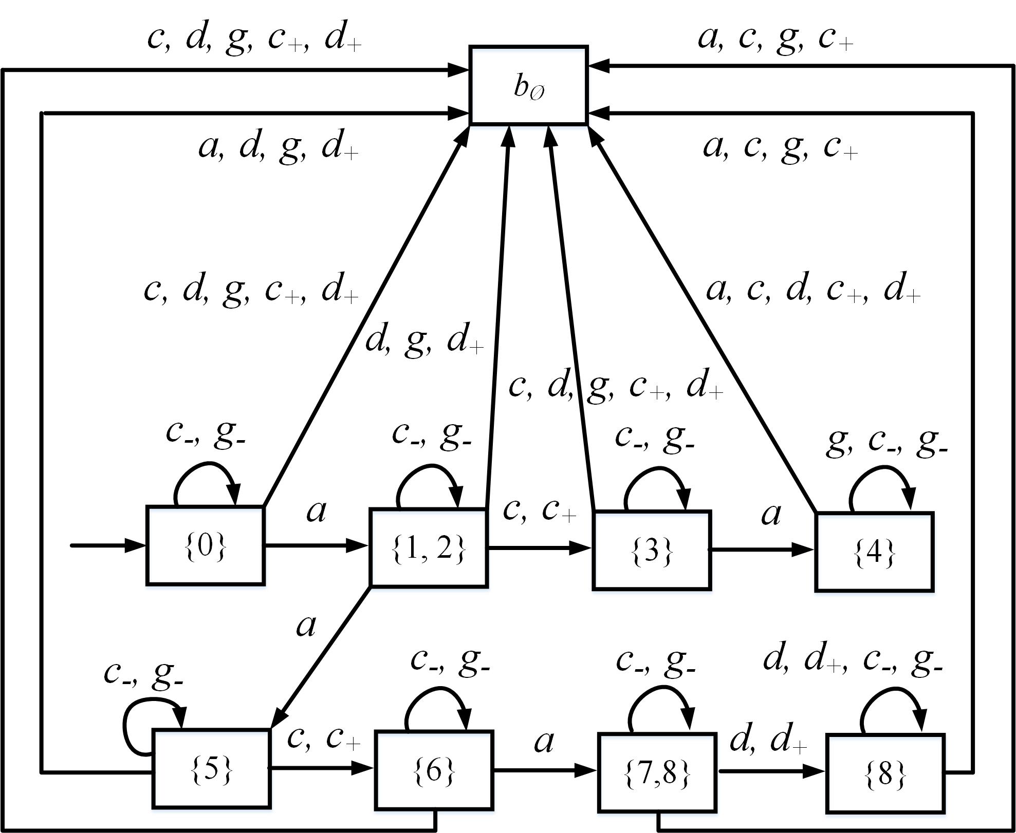
Since events $c,g\in E_{era}$, and there is a transition labeled $c$ from state $\{1,2\}$ to state $\{3\}$ in the observer of the plant $Obs(G)$, we add transitions labeled $c$ and $c_{-}$ from state $\{1,2\}$ to state $\{3\}$ in the attacker observer. Similar arguments can be used to explain transitions labeled $c$ and $c_{-}$ from state $\{5\}$ to state $\{6\}$, self-loops labeled $g$ and $g_{-}$ at state $\{4\}$. Then, since $c$, $d\in E_{ins}$, we add self-loops labeled $c_{+}$ and $d_{+}$ at all the states.  $\diamond$

The following proposition provides a characterization of the attacker observer.

1. (a)

   $L(Obs_{att}(G))=L({\mathcal{F}}_{\infty},G)$;

2. (b)

   $\forall s\in P(L(G))$, $\forall f_{\infty}\in{\mathcal{F}}_{\infty}$ with $w=f_{\infty}(s)\in E_{a}^{*}$:

   $$\delta_{att}^{*}(b_{0},w)=\delta_{obs}^{*}(b_{0},s).$$

Proof: (a) According to Algorithm 1, Step 2 implies that $L(Obs_{att}(G))$ contains all words that can be observed if no attack occurs. Correspondingly, according to the definition of attack function (Definition 3), the set of attack languages $L({\mathcal{F}}_{\infty},G)$ also contains these words since the attacker does not reduce the language of the plant.

Steps 3–9 guarantee that all attacks resulting from the cancellation of events in $E_{era}$ are considered. Correspondingly, according to the definition of attack function, each time the plant generates an event $e\in E_{era}$, then the attacker can erase it.

Finally, Steps 10–14 guarantee that all attacks resulting from the insertion of an arbitrarily large number of events in $E_{ins}$ are taken into account. Again, according to the definition of attack function, the attacker can insert any word $w_{+}\in E_{+}^{\leq n}$ whenever possible.

Thus, we can conclude that $L(Obs_{att}(G))=L({\mathcal{F}}_{\infty},G)$.

(b) We prove this by induction on the length of $s$. If $s=\varepsilon$, the result follows from the fact that, by definition of attack function, it is $f_{\infty}(\varepsilon)\in E_{+}^{\leq n}$, and by Steps 10–14, events in $E_{+}$ lead to self-loops in $Obs_{att}(G)$.

Let us now consider a generic word $s\in P(L(G))$ with length greater than one, written as $s=\overline{s}e$, where $\overline{s}\in P(L(G))$ and $e\in E_{o}$. Assume the result holds for $\overline{s}$. We prove that it also holds for $s=\overline{s}e$ considering the following two possible cases.

If $e\in E_{era}$, by the definition of attack function, $w\in\bigcup\limits_{f_{\infty}\in{\mathcal{F}}_{\infty}}f_{\infty}(\overline{s})\{e_{-},e\}E_{+}^{\leq n}$ is true. According to Steps 3–9, events $e$ and $e_{-}$ are dealt with in the same manner when defining the transition function $\delta_{att}$. Finally, as just pointed out, according to Steps 10–14, events in $E_{+}$ lead to self-loops in $Obs_{att}(G)$.

Finally, if $e\in E_{o}\setminus E_{era}$, by the definition of attack function, $w\in\bigcup\limits_{f_{\infty}\in{\mathcal{F}}_{\infty}}f_{\infty}(\overline{s})eE_{+}^{\leq n}$ is true. Thus the result follows from the fact that, according to Steps 10–14, events in $E_{+}$ lead to self-loops in $Obs_{att}(G)$ and events in $E_{o}$ are dealt with in the same manner in $Obs_{att}(G)$ and $Obs(G)$.  $\Box$

Now we discuss the computational complexity of constructing the attacker observer $Obs_{att}(G)$. Given a plant G with set of states X, the observer of the plant $Obs(G)$ can be constructed in $2^{|X|}$ steps. According to Algorithm 1, $Obs_{att}(G)$ has the same number of states as $Obs(G)$; thus the complexity of building $Obs_{att}(G)$ is $O(2^{|X|})$.

The attack model we are considering may change an observation $s$ into a corrupted observation $s^{\prime}$ which cannot be produced by the nominal plant. In this case the operator understands that the system is under attack. This can be formalized as follows.

In words, stealthiness requires that the set of words that an operator observes when the system is under attack is contained in the set of words the operator may observe when no attack occurs.

The operator observer $Obs_{opr}(G)$ generates two different sets of words. The first set includes all words on $E_{a}^{*}$ that may either result from an uncorrupted observation of the plant or from a corrupted observation which keeps the attacker stealthy. The second set of words includes all the previous words continued with a symbol in $E_{a}$ so that the resulting word is not consistent with an uncorrupted observation. While the words in the first set lead to a set of states that according to the operator are consistent with the perceived observation, those in the second set lead to a dummy state denoted as $b_{\emptyset}$. The operator observer $Obs_{opr}(G)$ can be constructed using Algorithm 2, as shown below.

According to Algorithm 2, the set of states $B_{opr}=B\cup\{b_{\emptyset}\}$ and the set of events $E_{a}$ are initially computed. Then, the transition function of $Obs_{opr}(G)$ is initialized at $\delta_{opr}=\delta_{obs}$. Indeed, events in $E_{o}$ are events actually occurring on the plant; when such events occur, the operator updates its state estimation according to the transition function of $Obs(G)$.

Furthermore, for all $e\in E_{ins}$ and for all $b\in B$, we impose $\delta_{opr}(b,e_{+})=\delta_{opr}(b,e)$. Indeed, the operator does not distinguish between events in $E_{+}$ and the corresponding events in $E_{ins}$. For all $e\in E_{era}$ and for all $b\in B$, we add self-loops $\delta_{opr}(b,e_{-})=b$. Indeed, events in $E_{-}$ correspond to no observation by the operator.

Finally, for all the events $e_{a}\in E_{a}$ that are not enabled at the generic state $b\in B$, let $\delta_{opr}(b,e_{a})=b_{\emptyset}$. As a result, for all $b\in B$ and for all $e_{a}\in E_{a}$, function $\delta_{opr}(b,e_{a})$ is defined. On the contrary, $\delta_{opr}(b_{\emptyset},e_{a})$ is undefined for all $e_{a}\in E_{a}$.

Since $c,d\in E_{ins}$ and there is a transition labeled $c$ from state $\{1,2\}$ to state $\{3\}$ in $Obs(G)$, we add transitions labeled $c$ and $c_{+}$ from state $\{1,2\}$ to state $\{3\}$ in the operator observer. Similar arguments can be used to explain the transitions labeled $c$ and $c_{+}$ from state $\{5\}$ to state $\{6\}$, the transitions labeled $d$ and $d_{+}$ from state $\{7,8\}$ to state $\{8\}$, and the self-loops labeled $d$ and $d_{+}$ at state $\{8\}$. Then, since $c$, $g\in E_{era}$, we add self-loops labeled $c_{-}$ and $g_{-}$ at all the states. Finally, we add all the missing transitions to the new state $b_{\emptyset}$, which has no output arc.  $\diamond$

To better characterize the properties of the operator observer, let us define two sets of words associated to an attack model as described in Subsection III-A.

In plain words, a stealthy word $w$ produces an observed word $s^{\prime}=\widehat{P}(w)$ which does not reveal the presence of the attacker because such an observation may have been produced by the plant. An exposing word is a non-stealthy word on $E_{a}$ whose strict prefixes are all stealthy: hence it reveals the presence of the attacker but only at the last step.

The following proposition provides a characterization of the operator observer.

1. (a)

   $L(Obs_{opr}(G))=W_{s}\cup W_{e}$;

2. (b)

   $\forall w\in L(Obs_{opr}(G))$: if $w\in W_{s}$, then $\delta_{opr}^{*}(b_{0},w)=\delta_{obs}^{*}(b_{0},\widehat{P}(w))$; if $w\in W_{e}$, then $\delta_{opr}^{*}(b_{0},w)=b_{\emptyset}$.

Proof: (a) Follows from Algorithm 2, and from the definitions of stealthy words, exposing words, and operator mask.

In more detail, Step 3 guarantees that all uncorrupted words belong to $L(Obs_{opr}(G))$. Steps 4–10 guarantee that, in $Obs_{opr}(G)$, events in $E_{+}$ lead to the same states of the corresponding events in $E_{ins}$. Steps 11–15 guarantee that, in $Obs_{opr}(G)$, events in $E_{-}$ lead to self-loops. The above steps guarantee that all the stealthy words $w\in W_{s}$ belong to $L(Obs_{opr}(G))$.

Finally, Steps 16–22 impose that, if after executing Steps 1–15, a certain event in $E_{a}$ is not already enabled at a certain state of $Obs_{opr}(G)$, then such an event is enabled at such a state and leads to state $b_{\emptyset}$, where no other event may be executed. These steps ensure that all the exposing words $w\in W_{e}$ belong to $L(Obs_{opr}(G))$.

(b) We prove this by induction on the length of $w$. If $w=\varepsilon$, the result holds being $\hat{P}(w)=\varepsilon$.

Consider now a word $w\in L(Obs_{opr}(G))$ with length greater than one. Assume $w\in W_{s}$, and let $w=w^{\prime}e_{a}$. Assume that the result holds for a generic $w^{\prime}\in W_{s}$. By definition of operator mask, if $e_{a}\in E_{o}\cup E_{+}$, then $\widehat{P}(w)=\widehat{P}(w^{\prime})e\in\widehat{P}(w^{\prime})\{e,\varepsilon\}$; otherwise $\widehat{P}(w)=\widehat{P}(w^{\prime})\in\widehat{P}(w^{\prime})\{e,\varepsilon\}$. Thus $\delta_{opr}^{*}(b_{0},w)=\delta_{opr}(\delta_{opr}^{*}(b_{0},w^{\prime}),e_{a})$. Then, $\delta_{obs}^{*}(b_{0},\widehat{P}(w))\!=\!\delta_{obs}(\delta_{obs}^{*}(b_{0}$, $\widehat{P}(w^{\prime})),e)$ if $e_{a}\in E_{o}\cup E_{+}$, and $\delta_{obs}^{*}(b_{0},\widehat{P}(w))=\delta_{obs}(\delta_{obs}^{*}(b_{0},\widehat{P}(w^{\prime})),\varepsilon)$ if $e_{a}\in E_{-}$.

According to Algorithm 2 the transition function of $Obs_{opr}(G)$ starting for a generic state $b\in B$ is defined in the same way in case of $e$ and $e_{+}$ (Steps 6 and 7), while it corresponds to a self-loop in the case of $e_{-}\in E_{-}$ (Step 13). As a result, we can conclude that $\delta_{opr}^{*}(b_{0},w)=\delta_{obs}^{*}(b_{0},\widehat{P}(w))$.

Finally, the last claim in (b) follows from the fact that, if $w\in W_{e}$, according to Algorithm 2, all the missing transitions end up in the new state $b_{\emptyset}$, thus $\delta_{opr}^{*}(b_{0},w)=b_{\emptyset}$.  $\Box$

Given a plant G with set of states X, the observer of the plant $Obs(G)$ can be constructed in $2^{|X|}$ steps. According to Algorithm 2, the operator observer $Obs_{opr}(G)$ has at most $2^{|X|}+1$ states; thus the complexity of constructing $Obs_{att}(G)$ is $O(2^{|X|})$.

References

- [1] D. Zhang, G. Feng, Y. Shi, and D. Srinivasan, “Physical safety and cyber security analysis of multi-agent systems: A survey of recent advances,” IEEE/CAA J. of Autom. Sinica, vol. 8, no. 2, pp. 319–333, Feb. 2021.
- [2] A. Rashidinejad, B. Wetzels, M. Reniers, L. Lin, Y. Zhu, and R. Su, “Supervisory control of discrete-event systems under attacks: An overview and outlook,” in Proc. 18th European Control Conference, Napoli, Italy, 2019, pp. 1732–1739.
- [3] M. Uma and G. Padmavathi, “A survey on various cyber attacks and their classification,” Int. J. of Network Security, vol. 15, no. 5, pp. 390–396, Sep. 2013.
- [4] F. Salahdine and N. Kaabouch, “Social engineering attacks: A survey,” Future Internet, vol. 11, no. 4, 2019.
- [5] A. Basit, M. Zafar, X. Liu, A. R. Javed, Z. Jalil, and K. Kifayat, “A comprehensive survey of AI-enabled phishing attacks detection techniques,” Telecommunication Syst., vol. 76, pp. 139–154, Jan. 2021.
- [6] X. Huang and J. Dong, “Reliable control policy of cyber-physical systems against a class of frequency-constrained sensor and actuator attacks,” IEEE Trans. Cybern., vol. 48, no. 12, pp. 3432–3439, Dec. 2018.
- [7] D. Rabehi, N. Meslem, and N. Ramdani, “Secure interval observer for linear continuous-time systems with discrete measurements subject to cyber-attacks,” in Proc. 4th Conference on Control and Fault Tolerant Systems, Casablanca, Morocco, 2019, pp. 336–341.
- [8] H. Liu, B. Niu, and J. Qin, “Reachability analysis for linear discrete-time systems under stealthy cyber attacks,” IEEE Trans. Autom. Control, vol. 66, no. 9, pp. 4444–4451, Sep. 2021.
- [9] W. Zhang, S. Mao, J. Huang, L. Kocarev, and Y. Tang, “Data-driven resilient control for linear discrete-time multi-agent networks under unconfined cyber-attacks,” IEEE Trans. Circuits Syst. I, vol. 68, no. 2, pp. 776–785, Feb. 2021.
- [10] D. Thorsley and D. Teneketzis, “Intrusion detection in controlled discrete event systems,” in Proc. IEEE 45th Annu. Conf. on Decision and Control, San Diego, USA, 2006, pp. 6047–6054.
- [11] F. A. Barbhuiya, M. Agarwal, S. Purwar, S. Biswas, and S. Nandi, “Application of stochastic discrete event system framework for detection of induced low rate TCP attack,” ISA Trans., vol. 58, pp. 474–492, Sep. 2015.
- [12] R. Fritz and P. Zhang, “Modeling and detection of cyber attacks on discrete event systems,” in Proc. of 14th Int. Workshop on Discrete Event Systems, Sorrento, Italy, 2018, pp. 285–290.
- [13] M. Agarwal, S. Biswas, and S. Nandi, “Discrete event system framework for fault diagnosis with measurement inconsistency: case study of rogue DHCP attack,” IEEE/CAA J. of Autom. Sinica, vol. 6, no. 3, pp. 789–806, May 2019.
- [14] Y. Ji, X. Yin, and S. Lafortune, “Enforcing opacity by insertion functions under multiple energy constraints,” Automatica, vol. 108, p. 108476, Oct. 2019.
- [15] L. K. Carvalho, Y.-C. Wu, R. Kwong, and S. Lafortune, “Detection and mitigation of classes of attacks in supervisory control systems,” Automatica, vol. 97, pp. 121–133, Nov. 2018.
- [16] P. M. Lima, M. V. S. Alves, L. K. Carvalho, and M. V. Moreira, “Security against network attacks in supervisory control systems,” in Proc. of the 20th IFAC World Congress, vol. 50, Toulouse, France, 2017, pp. 12 333–12 338.
- [17] M. Wakaiki, P. Tabuada, and J. P. Hespanha, “Supervisory control of discrete-event systems under attacks,” Dyn. Games and Appl., vol. 9, no. 4, pp. 965–983, Dec. 2019.
- [18] L. Lin and R. Su, “Synthesis of covert actuator and sensor attackers,” Automatica, vol. 130, p. 109714, Aug. 2021.
- [19] R. Meira-Góes, H. Marchand, and S. Lafortune, “Synthesis of supervisors robust against sensor deception attacks,” IEEE Trans. Autom. Control, DOI: 10.1109/TAC.2021.3051459.
- [20] Z. Jakovljevic, V. Lesi, and M. Pajic, “Attacks on distributed sequential control in manufacturing automation,” IEEE Trans. Ind. Informat., vol. 17, no. 2, pp. 775–786, Feb. 2021.
- [21] J. Yao, X. Yin, and S. Li, “On attack mitigation in supervisory control systems: a tolerant control approach,” in Proc. IEEE 59th Annu. Conf. on Decision and Control, Jeju Island, Republic of Korea, 2020, pp. 4504–4510.
- [22] Y. Wang and M. Pajic, “Supervisory control of discrete event systems in the presence of sensor and actuator attacks,” in Proc. IEEE 58th Annu. Conf. on Decision and Control, Nice, France, 2019, pp. 5350–5355.
- [23] D. You, S. Wang, M. Zhou, and C. Seatzu, “Supervisory control of Petri nets in the presence of replacement attacks,” IEEE Trans. Autom. Control, DOI: 10.1109/TAC.2021.3063699.
- [24] S. Zheng, S. Shu, and F. Lin, “Modeling and control of discrete event systems under joint sensor-actuator cyber attacks,” in Proc. 6th International Conference on Autom., Control and Robotics Engineering, Dalian, China, 2021, pp. 216–220.
- [25] Y. Tong, Z. Ma, Z. Li, C. Seatzu, and A. Giua, “Supervisory enforcement of current-state opacity with incomparable observations,” in Proc. of 13th Int. Workshop on Discrete Event Systems, Xi’an, China, 2016, pp. 313–318.
- [26] R. Meira-Góes, E. Kang, R. H. Kwong, and S. Lafortune, “Synthesis of sensor deception attacks at the supervisory layer of Cyber-Physical Systems,” Automatica, vol. 121, p. 109172, Nov. 2020.
- [27] P. M. Lima, L. K. Carvalho, and M. V. Moreira, “Detectable and undetectable network attack security of cyber-physical systems,” in Proc. of 14th Int. Workshop on Discrete Event Systems, Sorrento, Italy, 2018, pp. 179–185.
- [28] R. Su, “Supervisor synthesis to thwart cyber attack with bounded sensor reading alterations,” Automatica, vol. 94, pp. 35–44, Aug. 2018.
- [29] Q. Zhang, Z. Li, C. Seatzu, and A. Giua, “Stealthy attacks for partially-observed discrete event systems,” in Proc. of the 23th Int. Conf. on Emerging Technologies and Factory Autom., Turin, Italy, 2018, pp. 1161–1164.
- [30] K. Ding, Y. Li, D. E. Quevedo, S. Dey, and L. Shi, “A multi-channel transmission schedule for remote state estimation under Dos attacks,” Automatica, vol. 78, pp. 194–201, Apr. 2017.
- [31] L. Peng, L. Shi, X. Cao, and C. Sun, “Optimal attack energy allocation against remote state estimation,” IEEE Trans. Autom. Control, vol. 63, no. 7, pp. 2199–2205, Jul. 2018.
- [32] P. Cheng, Z. Yang, J. Chen, Y. Qi, and L. Shi, “An event-based stealthy attack on remote state estimation,” IEEE Trans. Autom. Control, vol. 65, no. 10, pp. 4348–4355, Oct. 2020.
- [33] P. J. G. Ramadge and W. M. Wonham, “The control of discrete event systems,” Proceedings of the IEEE, vol. 77, no. 1, pp. 81–98, Jan. 1989.
- [34] C. G. Cassandras and S. Lafortune, Introduction to discrete event systems. Springer, 2008.