Compressive Sensing Based Adaptive Active User Detection and Channel Estimation: Massive Access Meets Massive MIMOThanks: A part of this paper was presented in the 2018 6th IEEE Global Conference on Signal and Information Processing (GlobalSIP 2018) [1].Thanks: M. Ke and Z. Gao are with School of Information and Electronics, Beijing Institute of Technology, Beijing 100081, China (e-mail: kemalong@bit.edu.cn; gaozhen16@bit.edu.cn).Thanks: Y. Wu is with Department of Electronic Engineering, Shanghai Jiao Tong University, Shanghai 200240, China (e-mail: yongpeng.wu@sjtu.edu.cn).Thanks: X. Gao is with the National Mobile Communications Research Laboratory, Southeast University, Nanjing 210096, China (e-mail: xqgao@seu.edu.cn).Thanks: R. Schober is with the Institute for Digital Communications, Friedrich-Alexander-University Erlangen-Nnberg, Erlangen 91054, Germany (e-mail: robert.schober@fau.de).
Abstract
This paper considers massive access in massive multiple-input multiple-output (MIMO) systems and proposes an adaptive active user detection and channel estimation scheme based on compressive sensing. By exploiting the sporadic traffic of massive connected user equipments and the virtual angular domain sparsity of massive MIMO channels, the proposed scheme can support massive access with dramatically reduced access latency. Specifically, we design non-orthogonal pseudo-random pilots for uplink broadband massive access, and formulate the active user detection and channel estimation problems as a generalized multiple measurement vector compressive sensing problem. Furthermore, by leveraging the structured sparsity of the uplink channel matrix, we propose an efficient generalized multiple measurement vector approximate message passing (GMMV-AMP) algorithm to realize simultaneous active user detection and channel estimation based on a spatial domain or an angular domain channel model. To jointly exploit the channel sparsity presented in both the spatial and the angular domains for enhanced performance, a Turbo-GMMV-AMP algorithm is developed for detecting the active users and estimating their channels in an alternating manner. Finally, an adaptive access scheme is proposed, which adapts the access latency to guarantee reliable massive access for practical systems with unknown channel sparsity level. Additionally, the state evolution of the proposed GMMV-AMP algorithm is derived to predict its performance. Simulation results demonstrate the superiority of the proposed active user detection and channel estimation schemes compared to several baseline schemes.
Index Terms:
Massive access, active user detection, channel estimation, structured sparsity, message passing.I Introduction
Video streaming, social networking, and the emerging Internet-of-Things (IoT) accelerate the development of base stations (BSs) that enable connectivity for billions of user equipments (UEs) with massive data volumes [2]. However, reliable massive access for massive connectivity is not supported by the current wireless networks [3].
To guarantee the availability of resources and the quality of service in massive access scenarios, uplink systems have to provide ultra-reliable low-latency detection and channel estimation (CE) for active UEs [2]. Conventional grant-based random access (RA) protocols require control signaling and the scheduling of uplink access requests for granting of resources [4, 5, 6, 7]. The physical random access channel (PRACH) protocol of Long-Term Evolution is one example of grant-based protocols, and can be classified into two categories: contention-free RA and contention-based RA [4]. For contention-free RA, the BS first allocates UEs the dedicated preambles, which are then transmitted by the active UEs, and finally the BS responds to the requesting UEs without further contention resolution [5]. For contention-based RA, multiple active UEs first transmit preambles selected from a predefined sequence set to access the BS. Further contention resolution is required if multiple UEs choose the same preamble [6]. Unfortunately, for massive access, collisions are likely to occur as the number of potential UEs can be much larger than the number of available preambles. The authors in [7] proposed a strongest-user collision resolution protocol to resolve collisions in overloaded networks. However, such grant-based solutions generally suffer from high access latency and require complicated collision resolution schemes in massive access scenarios [8].
As a promising alternative, grant-free RA protocols have recently attracted significant attention, where each active UE directly transmits its pilots and data to the BS without waiting for permission [9, 10]. Allocating orthogonal channel resources (e.g., using orthogonal pilots as in [11]) can facilitate the detection of the active UEs at the BS and the estimation of their channels. However, for massive numbers of potential UEs, this approach fails due to the limited number of available orthogonal channels for a given channel coherence time. Fortunately, a key characteristic of massive access in future wireless networks is the sporadic traffic of the UEs, i.e., out of the many potential UEs, only a small number are activated and want to access the network in any given time interval [7].
Exploiting this sporadic traffic property, several compressive sensing (CS)-based grant-free RA schemes have been proposed, where the active user detection (AUD) is formulated as a sparse signal recovery problem [13, 12]. In [14, 15], two advanced CS-based multi-user detection schemes, which leverage the structured sparsity over multiple time slots for accurate support detection, were proposed to jointly detect the active UEs and to decode their data. To further exploit the a priori information about the transmitted discrete symbols for RA, the authors in [16] developed a joint approximate message passing (AMP) and expectation maximization (EM) algorithm to improve the detection performance of sparsely active UEs. Furthermore, the authors in [17] proposed a threshold aided block sparsity adaptive subspace pursuit algorithm, which enables improved sparse signal recovery. This work was also extended to cloud radio access networks (C-RANs) for efficient UE activity and data detection [18, 19]. However, the solutions in [14, 15, 16, 17, 18, 19] rely on the availability of perfect channel state information (CSI), which is difficult to obtain, especially for massive wireless-connected UEs.
To jointly perform AUD and CE for single-antenna BSs, blind detection of sparse code multiple access was proposed to support grant-free RA in massive access scenarios in [20]. For multi-antenna systems, the authors in [22] proposed a novel joint AUD and CE scheme, where the sparsity of delay-domain channel impulse response (CIR) is leveraged for facilitating CE. Particularly, in [22], by iteratively exchanging the active user information and CIR estimates, an identified user cancelation technique is further employed for enhanced performance. However, the delay-domain CIR sparsity highly depends on the channel environment and may be violated in some practical scenarios. Considering frequency-domain CE, a modified Bayesian compressive sensing (BCS)-based access scheme for uplink C-RANs was proposed in [21], where the structured sparsity over multiple receive antennas are exploited. To reduce the computational complexity, the authors in [23] and [24] developed an AMP-based scheme for AUD and CE for massive access in massive multiple-input multiple-output (MIMO) systems. However, the solutions in [23] and [24] require the full knowledge of the a priori distribution of the channels and the noise variance, which might not be available in practice. Besides, the work in [20, 21, 22, 23, 24] considers a narrow-band massive access scenario assuming single-carrier transmission.
Besides the aforementioned work, there are also related solutions that address the massive access problem with sparse user activity from information-theoretical perspectives [25, 26]. Especially in [26], the authors provided an elegant solution to support massive access with fully non-coherent detection.
In this paper, we consider massive access for the more challenging enhanced mobile broadband (eMBB) scenario, and investigate AUD and CE for uplink massive MIMO orthogonal frequency division multiplexing (OFDM) systems. By exploiting the sporadic traffic of the UEs and the virtual angular domain sparsity of massive MIMO channels, we develop a CS-based adaptive AUD and CE scheme. Specifically, a pilot design based on distributed CS (DCS) theory is proposed for broadband massive access. Moreover, the AUD and CE problems at the BS are formulated as a generalized multiple measurement vector (GMMV) CS problem [27]. By leveraging the structured sparsity of the uplink channel matrix, we propose a GMMV-AMP algorithm for efficient simultaneous AUD and CE based on a spatial domain or an angular domain channel model. To further improve performance, a Turbo-GMMV-AMP algorithm is proposed for detecting the active UEs and estimating their channels in an alternating manner. This forms the basis for an adaptive access scheme which allows the adaptation of the required access latency11 1 For grant-free massive access, the time slots consumed for transmitting the access pilot sequence contribute to the major part of the access latency. In this paper, we focus on the time slot overhead for pilot transmission. to the sparsity level of the uplink channel matrix, i.e., the maximum number of non-zero entries of its columns. Additionally, the state evolution (SE) of the proposed GMMV-AMP algorithm is derived to characterize its performance. Our main contributions can be summarized as follows.
- •
DCS theory-based pilot design tailored for multi-carrier systems: Previous work [14, 15, 16, 17, 18, 19, 20, 21, 22, 23, 24] mainly focuses on frequency-flat narrow-band massive access with single-carrier transmission. In contrast, we consider the more challenging massive access problem for eMBB, where OFDM is employed. Based on DCS theory [27], we design pseudo-random pilot sequences tailored for multi-carrier systems. Thereby, the structured channel sparsity for the different subcarriers is further leveraged to improve AUD and CE performance.
- •
GMMV-AMP algorithm: Exploiting the structured sparsity of the massive access channel matrix observed at multiple receive antennas and multiple subcarriers, the proposed GMMV-AMP algorithm facilitates efficient simultaneous AUD and CE. In particular, exploiting the EM algorithm, the GMMV-AMP algorithm can learn the unknown hyper-parameters of the a priori distribution of the channels and the noise variance.
- •
Turbo-GMMV-AMP algorithm: To jointly leverage the channel sparsity presented in both the spatial and the angular domains, this algorithm performs AUD and CE in an alternating manner for further enhanced performance. Compared with GMMV-AMP-based simultaneous processing methods and the state-of-the-art solutions, the proposed alternating approach will reap a significant reduction of access latency for massive access.
- •
CS-based adaptive AUD and CE: Most prior work [14, 15, 16, 17, 18, 19, 20, 21, 22, 23, 24] leverages the UEs’ sporadic traffic only to provide a fixed access latency. In contrast, the access latency for the proposed adaptive access scheme can be adapted to the actual sparsity level of the uplink massive access channel matrix for reliable AUD and CE.
Notations: Throughout this paper, scalar variables are denoted by normal-face letters, while boldface lower and upper-case letters denote column vectors and matrices, respectively. is the -th element of matrix ; and are the -th row vector and the -th column vector of matrix , respectively. The transpose, complex conjugate, and conjugate transpose operators are denoted by , , and , respectively. is the number of elements in set , denotes the set , and is the support set of a vector or a matrix. denotes the statistical expectation. denotes the empty set and is the zero matrix. Finally, denotes the complex Gaussian distribution of a random variable with mean and variance .
II System Model
In this section, we introduce the system model of the uplink massive access in massive MIMO-OFDM systems. Moreover, the sparsity properties of the massive access channel matrix presented in the spatial and the angular domains are further explained, respectively.
II-A Uplink Massive Access in Massive MIMO Systems
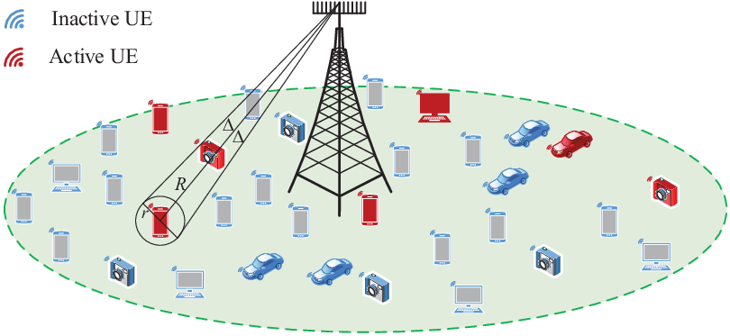
We consider the typical uplink massive access scenario in massive MIMO systems, as illustrated in Fig. 1. There are one BS equipped with an -antenna uniform linear array (ULA) and potential UEs, where is usually large (e.g., in [24]). OFDM with subcarriers is adopted to combat time dispersive channels, and pilots are uniformly allocated across the subcarriers. For the subchannel of the -th pilot subcarrier , the signal received at the BS from the -th UE in the -th time slot (or equivalently the -th OFDM symbol) can be expressed as
| (1) |
where is the subchannel associated with the -th UE, is the uplink access pilot of the -th UE, and denotes the additive white Gaussian noise (AWGN) at the BS for the -th pilot subcarrier and the -th time slot. Here, without loss of generality, we consider single-antenna UEs. For a typical massive access scenario, within a given time interval, only a small number of UEs are activated to access the BS. The UE activity indicator is denoted as , and is equal to 1 when the -th UE is active and 0 otherwise. Meanwhile, we define the set of active UEs as , and the number of active UEs is denoted by . Hence, the signal received at the BS from all active UEs for the -th pilot subcarrier and the -th time slot is given as follows
| (2) |
where and . By considering both the large-scale and the small-scale fading, we can model as , where is the large-scale fading caused by path loss and shadowing, and is the small-scale fading. For the -th pilot subcarrier, the subchannel of the -th UE is modeled as follows [32]
| (3) |
where is an integer, denotes the number of multi-path components (MPCs), and are the complex path gain and the path delay of the -th MPC, respectively, and is the two-sided bandwidth. The array response vector is given by , where . Here, is the angle of arrival (AOA) of the -th UE’s -th MPC, is the wavelength, and is the antenna spacing.
II-B Space-Frequency Structured Sparsity in Massive Access


Due to the sporadic traffic of the UEs, only a small number of UEs are active, i.e., . Thus, by defining , the channel vector observed at the -th receive antenna for the -th pilot subcarrier is sparse as
| (4) |
Moreover, all BS antennas exhibit the same sparsity,
| (5) |
We refer to this property as the spatial domain structured sparsity of massive access. Since the , are identical for all subchannels, the also exhibit a common sparsity pattern in the frequency domain as follows
| (6) |
The joint structured sparsity in (5) and (6) is referred to as the space-frequency structured sparsity of . To illustrate this structured sparsity in Fig.2(a), as an example, we assume that active UEs out of total UEs access the BS, which is equipped with antennas.
II-C Angular-Frequency Structured Sparsity in Massive MIMO
On the other hand, the BS is usually at high elevation with few scatterers around, whereas the UEs are typically located at low elevation in a rich local scattering environment far from the BS [27]. This scenario can be modeled using the classical one-ring channel model [28]. For a UE which is located at a distance of from the BS and surrounded by rich scatterers located within a radius of around the UE, the angular spread seen from the BS is expected to be very small as usually . This leads to sparsity of massive MIMO channels in the virtual angular domain [29, 30, 31]. Specifically, the virtual angular domain massive MIMO channel associated with the -th UE for the -th pilot subcarrier can be represented as
| (7) |
where the transformation matrix at the BS side is a unitary matrix. Here, depends on the geometry of the adopted array, and becomes the discrete Fourier transform matrix for a ULA with [32]. Due to the small and large , the channel vector is sparse, i.e.,
| (8) |
and this sparsity is clustered, as illustrated in Fig. 2(b). Moreover, since the spatial propagation characteristics of all wireless channels within the total bandwidth are similar, all subchannels associated with different subcarriers are affected by the same scatterers [27]. Consequently, the , have a common sparsity pattern in the frequency domain, i.e.,
| (9) |
We refer to the jointly structured sparsity in (8) and (9) as the angular-frequency structured sparsity of massive MIMO channels. Additionally, we further define the virtual angular domain channel matrix as , where . Considering the space-frequency structured sparsity described in (4)-(6), we further have , and
| (10) |
The illustration in Fig. 2(b) takes both the space-frequency structured sparsity of massive access and the angular-frequency structured sparsity of massive MIMO channels into account. These sparsity properties will be exploited in the remainder of this paper to achieve low-latency and highly-reliable AUD and CE performance.
III CS-Based Active User Detection and Channel Estimation Schemes
In this section, we detail the proposed CS-based AUD and CE schemes for massive access. First, a DCS-based pilot design is proposed for broadband massive access. Then, two simultaneous AUD and CE schemes are developed based on a spatial domain and an angular domain channel model, respectively. On this basis, the alternating AUD and CE schemes are further proposed for enhanced performance. Finally, the computational complexity of the proposed schemes will be analyzed.
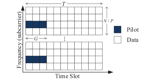
The frame structure of the uplink signals is illustrated in Fig. 3. A frame consists of time slots, where the first time slots include both pilots and data, and the remaining time slots are reserved for data transmission only. Here, we assume is smaller than the channel coherence time, and the activity of the UEs during the time slots remains unchanged. At the BS, the received signals in successive time slots for the -th pilot subcarrier are collected as
| (11) |
where , , , and . To avoid complicated scheduling protocols and the associated latencies, in RA, the active UE set (AUS) and the corresponding channel vectors , , have to be reliably estimated based on the noisy measurements and the known pilot matrices , which is equivalent to estimating based on (11). Due to the space-frequency structured sparsity of , the AUD and CE based on (11) can be formulated as a CS problem with . Moreover, considering the virtual angular domain sparsity shown in (8), we can further transform (11) as
| (12) |
where . Based on this, we develop two categories of AUD and CE schemes:
- •
- •
Alternating AUD and CE: Compared with in (11), the sparser in (12) will yield a better CE performance, but the common sparsity pattern across multiple columns of is destroyed. Therefore, the proposed alternating scheme leverages (11) for AUD and (12) for CE, i.e., (11) and (12) are alternately exploited to reap both the structured sparsity of and the enhanced sparsity of for further improved performance.
In the following, we will first discuss the pilot design and then explain the proposed AUD and CE schemes.
III-A DCS-Based Pilot Design for Broadband Massive Access
For the CS problems in (11) and (12), the RA pilot matrices , , serve as measurement matrix. The properties of the measurement matrix are crucial for guaranteeing reliable recovery of sparse channel matrices . Hence, the pilot signals should be carefully designed to guarantee reliable AUD and CE. The sparse signal recovery algorithms proposed in this paper are based on the family of AMP algorithms, which usually require independent and identically distributed (i.i.d.) Gaussian measurement matrices [33]. Hence, for the -th pilot subcarrier, the pilot associated with the -th UE in the -th time slot is generated from a standard complex Gaussian distribution, i.e., . Furthermore, the should be different for different pilot subcarriers to achieve diversity, which means that (11) and (12) are GMMV-CS models [27]. Compared to the conventional multiple measurement vector (MMV) problem [34], where identical pilots would be allocated to all pilot subcarriers, employing different pilot matrices across different pilot subcarriers can improve AUD and CE performance according to DCS theory [27].
III-B Simultaneous AUD and CE Schemes
For massive access, reliable inference of AUS and the corresponding , , from is challenging. In this subsection, we propose two simultaneous AUD and CE schemes, where a GMMV-AMP algorithm is developed to solve the CS problems in (11) and (12), respectively. Without loss of generality, we consider (11) first and focus on the -th pilot subcarrier. The obtained results can be easily extended to the model (12) and multiple pilot subcarriers.
1) Spatial Domain Simultaneous AUD and CE (Scheme 1): Define . The minimum mean square error (MMSE) estimate of is the posterior mean, which can be expressed as
| (13) |
In (13), the superscript and index in , , and are dropped to simplify the notation, and the marginal posterior distribution is given by
| (14) |
where denotes the collection of the . The joint posterior distribution in (14) can be computed according to the Bayesian rule as
| (15) | ||||
where is a normalization factor and is the a priori distribution of . Under the assumption of AWGN, the likelihood function in (15) is
| (16) |
where is the variance of the complex AWGN. In this paper, to characterize the sparsity of , we consider a flexible spike and slab a priori distribution for , i.e.,
| (17) | ||||
which can effectively capture the actual prior knowledge of the channel matrix [29, 30, 31]. In (17), is the sparsity ratio, i.e., the probability of being non-zero, is the Dirac delta function, and is the distribution of the non-zero entries. This distribution arises from the literature of AMP algorithm [35, 36], and has been successfully employed in various AMP-based channel estimation schemes [29, 30, 31].
The factorization in (15) can be represented by a bipartite graph, which consists of variable nodes, factor nodes, and the corresponding edges [37]. This suggests the use of message passing algorithms [37] to realize the MMSE estimator. As the messages for marginal posterior probabilities are difficult to compute for massive access, we resort to the AMP algorithm [33], which employs low-complexity heuristics for approximating .
Proposition 1
In the large system limit, i.e., , while and are fixed, the AMP algorithm decouples the matrix estimation problem based on (11) into scalar estimation problems. Considering this, the posterior distributions of , , are approximated as
| (18) | ||||
where denotes the -th iteration, and is a normalization factor. In (18), and are updated at the variable nodes of the bipartite graph as
| (19) | ||||
| (20) |
where and are updated at the factor nodes of the bipartite graph as
| (21) | ||||
| (22) |
Proof:
Please refer to the Appendix A. ∎
It is worth noticing that, although the proposed algorithms are developed from the large system limit (), in practice, they perform well even in the medium size problems, such as massive access with hundreds even thousands of UEs, which has been discussed in the literature of AMP algorithms [33, Sec. II], [41]. Moreover, we consider the widely used Gaussian a priori distribution for the channel gains, i.e., [29]. By exploiting this a priori model in (18), the posterior distribution of is obtained as
| (23) | ||||
where
| (24) | ||||
| (25) | ||||
| (26) |
and is referred to as the belief indicator. The posterior mean (62) and variance (63) can now be explicitly calculated as
| (27) | ||||
| (28) |
respectively.
Therefore, for the -th pilot subcarrier, the MMSE estimate of can be acquired by iteratively calculating (19)-(28) instead of solving the high-dimensional integrals in (14). The resulting procedure is referred to as the basic MMV-AMP algorithm. However, the basic MMV-AMP algorithm requires full knowledge of the a priori distribution of the channels and the noise variance , which may be difficult to obtain in practice. Hence, the EM algorithm is exploited to learn the unknown hyper-parameters, i.e., . The EM algorithm involves two steps
| (29) | ||||
| (30) |
where denotes the expectation conditioned on measurements with parameters , i.e., the expectation is with respect to the posterior distribution . There are two challenges in harnessing the EM algorithm: (a) the computation of is of high complexity and (b) the joint optimization of all elements of is difficult. Fortunately, in the large system limit with , the high complexity of calculating can be considerably reduced by using the approximation according to (18). Moreover, the incremental EM algorithm [38] can be used to simplify the joint optimization of all elements of , where is updated one element at a time and the other parameters are held constant. By setting the derivative of (29) with respect to one element of to zero, the update rules of the hyper-parameters are obtained as, :
| (31) | ||||
| (32) | ||||
| (33) | ||||
| (34) |
As the EM algorithm may converge to a local extremum of the likelihood function, the proper initialization of the hyper-parameters is crucial. Here, we use the following initialization [39], :
| (35) | ||||
| (36) | ||||
| (37) |
Here, and are the cumulative distribution function and the probability density function of the standard normal distribution, respectively, and is suggested in [39].
Equations (19)-(28) and (31)-(37) are the main EM steps incorporated into the MMV-AMP algorithm to learn the unknown hyper-parameters. However, the resulting overall algorithm is limited to the AUD and CE of a single pilot subcarrier. Hence, we extend the MMV-AMP algorithm to the GMMV-AMP algorithm (summarized in Algorithm 1), where the subchannel matrices , , for all pilot subcarriers are jointly estimated with different measurement matrices . Specifically, in lines 3-6, the messages are updated independently for all pilot subcarriers; in lines 4 and 5, a damping parameter is used to prevent the algorithm from diverging according to [40]; line 7 uses the incremental EM algorithm to learn the unknown hyper-parameters ; line 8 refines the update rule for the sparsity ratio to leverage the structured sparsity of the channel matrix for improved CS recovery. By contrast, the state-of-the-art AMP-based estimators in [23] and [24] require as a priori information.
In Algorithm 1, the sparsity ratio is the probability that the -th element of is non-zero. In line 7, is updated independently for all , , and according to (32), which indicates that the common sparsity pattern described in (5) and (6) is not exploited. To fully exploit the structured sparsity of the channel matrix, as discussed in Section II-B and illustrated in Fig. 2(a), we assume that the channel elements associated with the same UE have a common sparsity ratio, and further propose to refine as in line 8 of Algorithm 1, where we use
| (38) |
With the estimate of , the AUS and the corresponding channel vectors can be simultaneously acquired. Specifically, for AUD, we develop two UE activity detectors based on the and the belief indicators , , respectively, as follows. We first define a threshold function , where if , otherwise .
Definition 1
Based on , a channel gain-based activity detector (CG-AD) is proposed for AUD as follows
| (39) |
where , is the ratio of the minimum and maximum amplitudes of the channel coefficients, see [23, Sec. IV], and 22 2 If more than of the elements of are decided to be non-zero, the -th UE is declared active..
Proposition 2
In the large system limit, if a reliable estimate of is acquired after the convergence of the GMMV-AMP algorithm,
| (40) |
Proof:
Please refer to the Appendix B. ∎
Definition 2
Since the belief indicator tends to be 1 for and 0 for , we further design a belief indicator-based activity detector (BI-AD) as
| (41) |
For spatial domain simultaneous AUD and CE, we set to make the missed detection and false alarm probabilities identical, and the same as , we set based on empirical experience. Nevertheless, we note that the decisions of the CG-AD and BI-AD are not sensitive to the values of and 33 3 We found empirically via simulations for a wide range of system parameters that yields a high AUD performance.. Finally, if the -th UE is declared active, its channel is estimated as .
2) Angular Domain Simultaneous AUD and CE (Scheme 2): The GMMV-AMP algorithm designed for CS model (11) can be directly applied to model (12) for angular domain simultaneous AUD and CE by replacing and with and , respectively. Actually, (11) and (12) are equivalent signal models. Meanwhile, it is worth noticing that the channel matrix and exhibit two different forms of structured sparsity. Hence, the difference between the spatial domain and the angular domain schemes mainly lies in the different update rules (i.e., (38) and (42)) for refining the sparsity ratio in line 8 of Algorithm 1. Different from (11), both the space-frequency and the angular-frequency structured sparsity of the channel matrix are considered in (12), as has been discussed in Section II-C and illustrated in Fig. 2(b). Define the neighbors of as
| (42) | ||||
Due to the clustered sparsity and the structured sparsity described in (8)-(10), and the elements of tend to be simultaneously either zero or non-zero44 4 Here, we assume that no power leakage caused by the discrete Fourier transformation in (7) [29]. Otherwise, the channel would be approximately sparse.. Hence, when the GMMV-AMP algorithm is applied to (12), in line 8 is replaced by . Based on the estimate of , the can be acquired according to (7). Moveover, the active UEs can be detected via CG-AD in (39) based on or via BI-AD in (41) based on the belief indicators of , . However, as the common sparsity across multiple BS antennas is destroyed, it is challenging to find a suitable for BI-AD. Hence, we set to , where is the minimum number of non-zero elements of , . For AUD, our simulations in Section V reveal that, for Scheme 1 based on model (11), BI-AD is more reliable than CG-AD, but for Scheme 2 based on model (12), CG-AD is more reliable than BI-AD .
III-C Alternating AUD and CE Schemes
The simultaneous AUD and CE based on (11) or (12) can not fully exploit the enhanced sparsity of and the common sparsity pattern across the multiple columns of . Hence, we propose a Turbo-GMMV-AMP algorithm that performs AUD and CE in an alternating manner, where model (11) and model (12) are alternately exploited for enhanced performance. This facilitates the development of a CS-based adaptive AUD and CE scheme for practical massive access scenarios with unknown channel sparsity level.

1) Turbo-GMMV-AMP Algorithm (Scheme 3): This algorithm is summarized in Algorithm 2, and consists of module A and module B, as illustrated in Fig. 4. In the first turbo iteration (), module A determines a rough estimate of the AUS, where the GMMV-AMP algorithm is applied based on model (11) to obtain the belief indicators , . Even for small with poor estimation quality of , i.e., is smaller than a specific value rather than , the tend to be 0 for but 1 for after convergence of the GMMV-AMP algorithm, the related proof is similar to Appendix B. Hence, we use the BI-AD rather than CG-AD to acquire two AUS estimates with different reliability: a rough AUS with a lower threshold and a reliable AUS with a higher threshold , as shown in lines 6-13 in Algorithm 2, so that . Here, we set to 0.4 to obtain a low missed detection probability, and to 0.9 to avoid false alarm and to achieve reliable detection of the active UEs, i.e., the UEs in are active with high probability. These two AUSs, and , are passed on to module B.
In module B, with the rough AUS estimate , the angular domain channel vectors of the UEs in , i.e., , are estimated based on the model in (12) as
| (43) |
where and are sub-matrices of and , respectively, , is the set of all potential UEs, and denotes the difference set of sets and . To reduce the power of , is desirable, i.e., a low missed detection probability. The dimension of the uplink channel matrix for CE is reduced by considering only the UEs in . Furthermore, the low-dimensional channel matrix is still sparse due to the angular-frequency structured sparsity of massive MIMO channels. Hence, we can estimate , by applying the GMMV-AMP algorithm to (43), see line 16 of Algorithm 2. Moreover, the signals received from the UEs in , a subset of , are removed to enhance the sparsity of the uplink massive access channel matrix for AUD. The residual received signals are computed in lines 17 and 18, and are passed on to module A.
In the following turbo iterations (), the AUD problem in module A is to recover based on the following model
| (44) |
where contains the residual received signals in the -th turbo iteration, , and is defined as, , while . To prevent the GMMV-AMP algorithm from diverging, we only remove the signals received from a part of the UEs in , i.e., (e.g. ). Modules A and B will be executed iteratively. Since the become sparser and the channels of the UEs in are iteratively re-estimated as the turbo iterations proceed, the and the corresponding channels are constantly refined. Therefore, compared to the simultaneous processing approaches in Section III-B, the proposed alternating approach facilitates more reliable AUD and CE with significantly smaller , which means a dramatic reduction of access latency.
2) CS-Based Adaptive AUD and CE (Scheme 4): For practical systems, the UE activity and the channel environment are time-varying. As a result, the sparsity level of the uplink massive access channel matrix may change over time. If the channel matrix is relatively sparse, a small time slot overhead is sufficient to acquire accurate AUS and CSI estimates, while if the channel matrix is relatively dense, a large is required to guarantee reliable sparse signal recovery. This motivates us to propose a CS-based adaptive AUD and CE scheme, as shown in Algorithm 3, to adaptively adjust to facilitate low-latency and high-reliability AUD and CE. Algorithm 3 can be summarized as follows.
- •
Step 1: In each time slot, all active UEs transmit non-orthogonal RA pilots to the BS. The pilots are pre-designed based on DCS theory and known to the system.
- •
Step 2: The BS collects the received signals over multiple successive time slots, and the Turbo-GMMV-AMP algorithm is utilized to alternately acquire the AUS and CSI estimates, see lines 3-5 of Algorithm 3. Besides, the estimation reliability is evaluated based on a pre-specified criterion, see line 8 of Algorithm 3.
- •
Step 3: If the criterion is met, the outcome of the evaluation is informed to all UEs, and the active UEs stop transmitting pilots and start to transmit their data to the BS without scheduling permission. Otherwise, Step 1 is repeated until the received signals collected at the BS are sufficient to meet the evaluation criterion.
Here, based on CS theory, is desirable, and is suggested in [27, Sec. V].
III-D Computational Complexity Analysis
For the practical implementation of the algorithms, the related computational complexity determines the hardware cost and the power consumption for processing. Hence, the complexity analysis for the proposed algorithms is an important issue, especially for massive connectivity with large scale systems.
Table I compares the complexity of the proposed GMMV-AMP algorithm and Turbo-GMMV-AMP algorithm, as well as the conventional greedy CS recovery algorithms, i.e., generalized subspace pursuit (GSP) [43], simultaneous orthogonal matching pursuit (SOMP) [42], and distributed sparsity adaptive matching pursuit DSAMP [27, 44], in terms of the number of the required complex multiplications in each iteration for AUD and CE. Obviously the matrix inversion implemented in three greedy CS recovery algorithms for least square operation contributes to most of the computational complexity. Hence, three greedy methods have the same order of computational complexity, i.e., in order of cubic magnitude of the number of active UEs . By contrast, the complexity of the proposed GMMV-AMP and Turbo-GMMV-AMP algorithms increases linearly with , and . Hence, for massive access scenarios with large , the proposed algorithms can be more computationally efficient.
IV State Evolution
SE is a framework for analyzing the performance of AMP algorithms in the large system limit where [41]. In this section, we harness SE to characterize the mean square error (MSE) performance of the proposed GMMV-AMP algorithm. The MSE of the estimation and the variance of the estimated channels are defined as
| (45) | ||||
| (46) |
respectively. Based on the derivations in Appendix A, the GMMV-AMP algorithm can be explained intuitively. For the -th pilot subcarrier, the proposed GMMV-AMP algorithm decouples the matrix estimation problem in (11) into independent scalar estimation problems, as
| (47) |
where index and superscript are omitted for notational simplicity, is the equivalent measurement of in the -th iteration, and denotes the effective noise.
Proposition 3
Define a scalar random variable . Then, we have , , and the posterior distribution of can be expressed as
| (48) |
where
| (49) |
and . Hence, and are updated as
| (50) | ||||
| (51) |
where and . Therefore, defining a scalar random variable following the same distribution as the channel coefficient, i.e., , and in the GMMV-AMP algorithm can be calculated as in (49), and and can be obtained from (50) and (51).
Proof:
Please refer to the Appendix C. ∎
Since the a priori distribution does not take the structured sparsity of channel matrix into consideration, the scalar SE in (49)-(51) can not accurately analyze the MSE performance of the proposed GMMV-AMP algorithm. Hence, we use Monte Carlo simulation to carry out the SE, so that (50) and (51) are simplified and the exploitation of the structured sparsity is also taken into into account. In contrast to the conventional AMP algorithms in [23] and [24], which assume full knowledge of the a priori distribution of the channels and the noise variance, the SE for the proposed GMMV-AMP algorithm also needs to track the update rules of the hyper-parameters in (31)-(33), and [29]
| (52) |
where is the actual noise variance. The SE of the proposed GMMV-AMP algorithm is summarized in Algorithm 4.
V Simulation Results
For the presented simulation results, we assume the BS employs a ULA with antennas, potential UEs are randomly distributed in the cell with radius 1 km, and () UEs are active unless otherwise specified. Furthermore, the carrier frequency is 2 , the bandwidth is , and the received SNR is 30 . The system adopts OFDM for massive access in an eMBB scenario, where subcarriers and a cyclic prefix of length are employed. pilots are uniformly allocated to the subcarriers [27]. We consider the one-ring channel model with limited angular spread [28], so that each UE’s massive MIMO channel exhibits clustered sparsity in the virtual angular domain. The large scale fading is given by the standard Log-distance path loss model as with distance measured in km. The small scale fading channel is generated by (3), where varies from 8 to 40 [29], the related AOAs are generated within an angular spread varying from to so that the effective sparsity level in virtual angle domain varies from 8 to 14, , and is randomly and uniformly selected from . Furthermore, , , , and the simulation results are obtained by averaging over simulation runs unless otherwise specified.
| Scheme | Model | Algorithm | ||||||
| Simultaneous AUD and CE | Scheme 1 | (11) | GMMV-AMP | fixed | ||||
| Scheme 2 | (12) | GMMV-AMP | fixed | |||||
| Alternating AUD and CE | Scheme 3 | (11) and (12) | Turbo-GMMV-AMP | fixed | ||||
| Scheme 4 | (11) and (12) | Turbo-GMMV-AMP | adaptive | |||||
|
(11) |
|
fixed | |||||
An overview of the proposed Schemes 1-4 and the considered baseline schemes, GSP [43], SOMP [42], and DSAMP [27], is presented in Table II. For performance evaluation, we consider the detection error probability for AUD and the MSE for CE, which are respectively defined as
| (53) |
Here, to reduce computational complexity, for Schemes 1-4, only out of pilot subcarriers are used to estimate AUS and the corresponding channels. The remaining pilot subchannels of the active UEs can be easily estimated by applying the GMMV-AMP algorithm to (43) given .

Fig. 5 verifies the superiority of the proposed DCS-based pilot design for broadband massive access based on Scheme 1. The quality of the pilots is evaluated in terms of the success rate, which is defined as the ratio of the number of simulation runs with to the total number of simulation runs. Fig. 5 shows that, as expected, employing different for different improves the success rate. Moreover, the performance is further improved when massive MIMO and larger are employed, since the structured sparsity of is leveraged.

Fig. 6 examines the AUD performance of Scheme 1, where the performances of three state-of-the-art GMMV-CS algorithms are shown as benchmarks. As can be observed, the GMMV-AMP algorithm outperforms the other three algorithms. Hence, the access latency can be considerably reduced for a given target . For example, for and , the GSP-based scheme requires to achieve , whereas Scheme 1 with BI-AD needs only , which indicates a reduction of approximately in the access latency. Moreover, Scheme 1 can achieve a better detection performance by equipping more antennas at the BS and/or utilizing larger , since a larger and/or can enhance the space-frequency structured sparsity shown in Fig. 2(a). However, this improvement becomes negligible when and are sufficiently large.
In Fig. 6, we further compare the performance of CG-AD and BI-AD. For or , CG-AD and BI-AD have similar performance. However, when and , BI-AD outperforms CG-AD, as CG-AD suffers from a detection error floor. The reason for this behavior is that when there are sufficiently many measurements for reliable CS recovery, the belief indicator takes values of 0 and 1, but the estimated channel gain takes the true value of . Hence, based on the threshold function , BI-AD can reliably determine whether is zero or not, while for CG-AD, missed detections and false alarms can not be avoided, which may lead to a detection error floor. Clearly, for Scheme 1, BI-AD is more reliable than CG-AD for AUD.

Fig. 7 depicts the CE MSE performance of Scheme 1 and the three state-of-the-art GMMV-CS algorithms also considered in Fig. 6. The oracle least square (LS) estimator with known AUS is used as performance upper bound [27]. When is sufficiently large, both Scheme 1 and the three baseline schemes approach the oracle LS performance bound, since is accurately estimated in this case, and the CE problem is reduced to an oracle LS problem. However, for , Scheme 1 outperforms the three baseline algorithms, and its performance improves when and/or increase. Besides, the MSE performance of Scheme 1 is accurately predicted by SE. Here, an important observation is that when , both Scheme 1 and the oracle LS estimator can not perform reliable CE. This suggests that is required for reliable CE in (11). Hence, the reduction of is limited to , which is identical to the sparsity level of the column vectors in . This motivates Scheme 2 for simultaneous AUD and CE, where the sparsity level of the channel matrix, defined as , is less than .

Fig. 8 compares the AUD performance of Scheme 1 and Scheme 2. For , Scheme 1 outperforms Scheme 2 for both BI-AD and CG-AD, respectively. In contrast, for , Scheme 2 achieves a much better AUD performance than Scheme 1 when . This is because is sparser than , i.e., , and the required for reliable AUD and CE in Scheme 2 mainly depends on rather than . However, the virtual angular domain sparsity weakens the common sparsity pattern across multiple columns of . Therefore, if the BS has a small number of antennas, e.g., , Scheme 1 outperforms Scheme 2 by leveraging the common sparsity observed at different BS antennas. However, when becomes large, Scheme 2 can considerably reduce the required for reliable AUD and CE compared to Scheme 1. In addition, BI-AD in Scheme 2 suffers from an obvious detection error floor, which indicates that for Scheme 2, CG-AD is more reliable than BI-AD for detection of the active UEs. Fig. 9 compares the CE MSE performance of Scheme 1 and Scheme 2, which again verifies the superiority of Scheme 2 for massive MIMO systems. The theoretical SE accurately predicts the MSE.


Fig. 10 and Fig. 11 compare the MSE and performance of Schemes 1-4, respectively. The details of Scheme 4 are shown in Algorithm 3. Given and , an initial time slot overhead of
| (54) | ||||
is adopted. For different simulation runs, the varying yields a different sparsity level for , i.e., different . The results and the consumed , i.e., the overhead, are recorded after the pre-defined criterion in line 8 of Algorithm 3 is met. For very low time slot overheads, i.e., , both Scheme 1 and Scheme 2 have a poor performance. This is because for these schemes, leads to extremely insufficient measurements. By contrast, Scheme 3 using the proposed Turbo-GMMV-AMP algorithm can achieve a much better AUD and CE performance than Scheme 1 and Scheme 2, which confirms its superiority in reducing access latency. Finally, Scheme 4, i.e., the proposed CS-based adaptive AUD and CE scheme, adaptively adjusts the overhead to achieve satisfactory AUD and CE performance. In Fig. 11, for Scheme 4, the percentage of simulation runs requiring the given time slot overhead is provided. This reveals that of the simulation runs require overheads of , and the corresponding MSE performance is much better than those for Schemes 1-3.
Fig. 12 further compares the AUD and CE performance of Scheme 3 and Scheme 4 for different number of active UEs . The proposed Scheme 4 adaptively adjusts the time slot overhead to guarantee reliable AUD and CE for different . However, Scheme 3 employs a fixed overhead and suffers from poor performance when becomes large. This means that some of the active UEs will not be able to access the network. Hence, for practical systems with time-varying UE activity, the superiority of the proposed CS-based adaptive AUD and CE scheme is evident.
VI Conclusion
This paper investigates new methods for facilitating massive access in massive MIMO systems, which leverage the sporadic traffic of the UEs and the virtual angular domain sparsity of massive MIMO channels to dramatically reduce the access latency. The space-frequency structured sparsity of the channel matrix in the spatial domain improves the AUD performance, while the angular-frequency structured sparsity of the channel matrix in the angular domain improves the CE performance. Therefore, joint AUD and CE schemes exploiting only spatial domain or only angular domain channel model can not take full advantage of the sparsity properties of massive access in massive MIMO systems. This motivates the derivation of the proposed Turbo-GMMV-AMP algorithm, which achieves a significant performance improvement by performing AUD based on a spatial domain channel model and CE based on an angular domain channel model in an alternating manner. Furthermore, for practical systems, where the number of active UEs is not known, the proposed CS-based adaptive AUD and CE scheme can adjust the time slot overhead to realize ultra-reliable low-latency massive access.
Appendix A Proof of the Proposition 1
The factorization in the joint posterior probability (15) can be represented by a bipartite graph, which motivates the application of the sum-product (SP) algorithm to realize the MMSE estimator [37]. As the bipartite graph consists of independent subgraphs, we only discuss the -th subgraph in the following derivations, and the antenna index is dropped for notational simplicity. For the -th subgraph, we define variable nodes , factor nodes of the likelihood function , and edges . The update rules for the messages associated to the edges are [33]
| (55) | ||||
| (56) |
where , , denotes the -th iteration, and denotes equality up to a constant scale factor.
One practical hurdle for the large-scale implementation of the SP algorithm lies in the required evaluation of high-dimensional integrals for calculation of messages . This leads to an unacceptably high complexity. However, a key observation is that, in the large system limit with , the messages can be approximated by Gaussian distributions [33]. Since the random variables are independently complex Gaussian distributed, random variable follows a complex Gaussian distribution , with mean and variance given as
| (57) |
where and are the mean and variance of message , respectively. Hence, the messages can be approximated as
| (58) |
Further, the posterior distribution of is calculated as
| (59) | ||||
where
| (60) |
It is convenient to introduce a family of densities
| (61) |
where is a normalization constant. The corresponding mean and variance are
| (62) | ||||
| (63) |
respectively. Define , with and . The messages can be approximated as
| (64) |
where
| (65) | ||||
| (66) |
At this point, the messages and have been approximated as Gaussian densities. However, the computational complexity is still high when the system is large, since the number of messages scales with the number of potential UEs . In order to reduce the number of messages in the -th iteration, we can further simplify the update rules by making some approximations. Defining , , we can rewrite (57) as
| (67) |
Substituting (67) into (64) and ignoring terms approximated as 0 in the large system limit [33], the update rules at the variable nodes and the factor nodes can be approximated as in (19)-(22). Finally, the posterior distribution of is given by (18).
Appendix B Proof of the Proposition 2
If a reliable estimate of is acquired after the convergence of the GMMV-AMP algorithm, the variance of the posterior distribution of tends to be zero, i.e., , thus,
| (68) |
Therefore, in (19) is calculated as
| (69) |
Here, approximation is because the pilots are generated from an i.i.d standard complex Gaussian distribution, i.e., , thus . In the large system limit, as , . For a given realization of the massive access channel matrix , defining , in (20) is given as
| (70) |
Hence, substituting (69) and (70) into (26), for , we have
| (71) |
while for ,
| (72) | ||||
which yields
| (73) |
Appendix C Proof of the Proposition 3
Here, for simplicity of derivation, we focus on the -th subgraph only and drop the antenna index , as in Appendix A. The derivation is based on (11), and can be easily extended to model (12), thus we have
| (74) |
Substituting (57) and (74) into (60), is computed as
| (75) | ||||
In (75), approximation is because the term is approximately independent of in the large system limit with , which has been proven in [33]. Define
| (76) |
Since , , and is independent of , follows a complex Gaussian distribution according to the central limit theorem as . Moreover, by substituting (45) into (76), we find the mean and the variance of are 0 and , respectively. Hence,
| (77) |
where . Meanwhile, by substituting (46) into in (60), we can obtain
| (78) |
Hence, the Proposition 2 is proven.
References
- [1] M. Ke, Z. Gao, Y. Wu, and X. Meng, “Compressive massive random access for massive machine-type communications (mMTC),” in Proc. IEEE Global Conf. Signal Inform. Process. (GlobalSIP), Anaheim, USA, Nov. 2018, pp. 156-160.
- [2] F. Boccardi, R. W. Heath, A. Lozano, T. L. Marzetta, and P. Popovski, “Five disruptive technology directions for 5G,” IEEE Commun. Mag., vol. 52, no. 2, pp. 74-80, Feb. 2014.
- [3] C. Bockelmann, N. K. Pratas, G. Wunder, S. Saur, et al, “Towards massive connectivity support for scalable mMTC communications in 5G networks,” IEEE Access., vol. 6, pp. 28969-28992, May. 2018.
- [4] T. Kim, I. Bang, and D. K. Sung, “An enhanced PRACH preamble detector for cellular IoT communications,” IEEE Commun. Lett., vol. 21, no. 12, pp. 2678-2681, Dec. 2017.
- [5] M. Hasan, E. Hossain, and D. Niyato, “Random access for machine-to-machine communication in LTE-advanced networks: Issues and approaches,” IEEE Commun. Mag., vol. 51, no. 6, pp. 86-93, Jun. 2013.
- [6] H. Han, Y. Li, and X. Guo, “A graph-based random access protocol for crowded massive MIMO systems,” IEEE Trans. Wireless Commun., vol. 16, no. 11, pp. 7348-7361, Nov. 2017.
- [7] E. Björnson, E. de Carvalho, J. H. Sørensen, E. G. Larsson, and P. Popovski, “A random access protocol for pilot allocation in crowded massive MIMO systems,” IEEE Trans. Wireless Commun., vol. 16, no. 4, pp. 2220-2234, Apr. 2017.
- [8] A. Laya, L. Alonso, and J. Alonso-Zarate, “Is the random access channel of LTE and LTE-A suitable for M2M communications? A survey of alternatives,” IEEE Commun. Surveys Tuts., vol. 16, no. 1, pp. 4-16, 1st Quart., 2014.
- [9] Z. Zhang, X. Wang, Y. Zhang, and Y. Chen, “Grant-free rateless multiple access: A novel massive access scheme for internet of things,” IEEE Commun. Lett., vol. 20, no. 10, pp. 2019-2022, Oct. 2016.
- [10] L. Liu, E. G. Larsson, W. Yu, P. Popovski, C. Stefanovic, and E. de Carvalho, “Sparse signal processing for grant-free massive connectivity: A future paradigm for random access protocols in the internet of things,” IEEE Signal Process. Mag., vol. 35, no. 5, pp. 88-99, Sep. 2018.
- [11] M. Simko, P. S. R. Diniz, Q. Wang, and M. Rupp, “Adaptive pilot-symbol patterns for MIMO-OFDM systems,” IEEE Trans. Wireless Commun., vol. 12, no. 9, pp. 4705-4715, Sep. 2013.
- [12] K. Senel and E. G. Larsson, “Grant-free massive MTC-enabled massive MIMO: A compressive sensing approach,” IEEE Trans. Commun., vol. 66, no. 12, pp. 6164-6175, Dec. 2018.
- [13] B. Shim and B. Song, “Multiuser detection via compressive sensing,” IEEE Commun. Lett., vol. 16, no. 7, pp. 972-974, Jul. 2012.
- [14] B. Wang, L. Dai, T. Mir, and Z. Wang, “Joint user activity and data detection based on structured compressive sensing for NOMA,” IEEE Commun. Lett., vol. 20, no. 7, pp. 1473-1476, Jul. 2016.
- [15] B. Wang, L. Dai, Y. Zhang, T. Mir, and J. Li, “Dynamic compressive sensing-based multi-user detection for uplink grant-free NOMA,” IEEE Commun. Lett., vol. 20, no. 11, pp. 2320-2323, Nov. 2016.
- [16] C. Wei, H. Liu, Z. Zhang, J. Dang, and L. Wu, “Approximate message passing-based joint user activity and data detection for NOMA,” IEEE Commun. Lett., vol. 21, no. 3, pp. 640-643, Mar. 2017.
- [17] Y. Du, C. Cheng, B. Dong, Z. Chen, X. Wang, J. Fang, and S. Li, “Block-sparsity-based multiuser detection for uplink grant-free NOMA,” IEEE Trans. Wireless Commun., vol. 17, no. 12, pp. 7894-7909, Dec. 2018.
- [18] X. Rao and V. K. N. Lau, “Distributed fronthaul compression and joint signal recovery in cloud-RAN,” IEEE Trans. Signal Process., vol. 63, no. 4, pp. 1056-1065, Feb. 2015.
- [19] J. Liu, A. Liu, and V. K. N. Lau, “Compressive interference mitigation and data recovery in cloud radio access networks with limited fronthaul,” IEEE Trans. Signal Process., vol. 65, no. 6, pp. 1437-1446, Mar. 2017.
- [20] A. Bayesteh, E. Yi, H. Nikopour, and H. Baligh, “Blind detection of SCMA for uplink grant-free multiple-access,” in Proc. 11th Int. Symp. Wireless Commun. Syst. (ISWCS), Aug. 2014, pp. 853-857.
- [21] X. Xu, X. Rao, and V. K. N. Lau, “Active user detection and channel estimation in uplink C-RAN systems,” in Proc. Int. Conf. Commun. (ICC), Jun. 2015, pp. 2727-2732.
- [22] S. Park, H. Seo, H. Ji, and B. Shim, “Joint active user detection and channel estimation for massive machine-type communications,” in Proc. IEEE Int. Workshop Signal Process. Adv. Wireless Commun. (SPAWC), Sapporo, Japan, Jul. 2017, pp. 1-5.
- [23] Z. Chen, F. Sohrabi, and W. Yu, “Sparse activity detection for massive connectivity,” IEEE Trans. Signal Process., vol. 66, no. 7, pp. 1890-1904, Apr. 2018.
- [24] L. Liu and W. Yu, “Massive connectivity with massive MIMO-Part I: Device activity detection and channel estimation,” IEEE Trans. Signal Process., vol. 66, no. 11, pp. 2933-2946, Jun. 2018.
- [25] Y. Polyanskiy, “A perspective on massive random-access,” in Proc. IEEE Int. Symp. Inform. Theory. (ISIT), Jun. 2017, pp. 2523-2527.
- [26] A. Fengler, G. Caire, P. Jung, and S. Haghighatshoar, “Massive MIMO unsourced random access,” arXiv preprint arXiv:1901.00828, 2019.
- [27] Z. Gao, L. Dai, Z. Wang, and S. Chen, “Spatially common sparsity based adaptive channel estimation and feedback for FDD massive MIMO,” IEEE Trans. Signal Process., vol. 63, no. 23, pp. 6169-6183, Dec. 2015.
- [28] J. Nam, A. Adhikary, J. Ahn, and G. Caire, “Joint spatial division and multiplexing: Opportunistic beamforming, user grouping and simplified downlink scheduling,” IEEE J. Sel. Topics Signal Process., vol. 8, no. 5, pp. 876-890, Oct. 2014.
- [29] X. Lin, S. Wu, C. Jiang, L. Kuang, J. Yan, and L. Hanzo, “Estimation of broadband multiuser millimeter wave massive MIMO-OFDM channels by exploiting their sparse structure,” IEEE Trans. Wireless Commun., vol. 17, no. 6, pp. 3959-3973, Jun. 2018.
- [30] X. Lin, S. Wu, L. Kuang, Z. Ni, X. Meng, and C. Jiang, “Estimation of sparse massive MIMO-OFDM channels with approximately common support,” IEEE Commun. Lett., vol. 21, no. 5, pp. 1179-1182, May. 2017.
- [31] J. Zhang, X. Yuan, and Y. A. Zhang, “Blind signal detection in massive MIMO: Exploiting the channel sparsity,” IEEE Trans. Commun., vol. 66, no. 2, pp. 700-712, Feb. 2018.
- [32] Y. Zhou, M. Herdin, A. M. Sayeed, and E. Bonek, “Experimental study of MIMO channel statistics and capacity via the virtual channel representation,” Univ. Wisconsin-Madison, Madison, WI, USA, Tech. Rep, 2007.
- [33] D. L. Donoho, A. Maleki, and A. Montanari, “Message passing algorithms for compressed sensing: I. motivation and construction,” in Proc. Inf. Theory Workshop. (ITW), Jan. 2010, pp. 1-5.
- [34] J. Chen and X. Huo, “Theoretical results on sparse representations of multiple-measurement vectors,” IEEE Trans. Signal Process., vol. 54, no. 12, pp. 4634-4643, Dec. 2006.
- [35] J. P. Vila and P. Schniter, “Expectation-maximization gaussian-mixture approximate message passing,” IEEE Trans. Signal Process., vol. 61, no. 19, pp. 4658-4672, Oct. 2013.
- [36] X. Meng, S. Wu, M. R. Andersen, J. Zhu, and Z. Ni, “Efficient recovery of structured sparse signals via approximate message passing with structured spike and slab prior,” IEEE China Commun., vol. 15, no. 6, pp. 1-17, Jun. 2018.
- [37] F. R. Kschischang, B. J. Frey, and H. A. Loeliger, “Factor graph and the sum-product algorithm,” IEEE Trans. Inform. Theory., vol. 47, no. 2, pp. 498-519, Feb. 2001.
- [38] R. M. Neal and G. E. Hinton, “A view of the EM algorithm that justifies incremental, sparse, and other variants,” in Learning in graphical models., Springer, 1998, pp. 355-368.
- [39] S. Wu, Z. Ni, X. Meng, and L. Kuang, “Block expectation propagation for downlink channel estimation in massive MIMO systems,” IEEE Commun. Lett., vol. 20, no. 11, pp. 2225-2228, Nov. 2016.
- [40] S. Rangan, P. Schniter, and A. Fletcher, “On the convergence of approximate message passing with arbitrary matrices,” in Proc. Int. Symp. Inform. Theory. (ISIT), Jun. 2014, pp. 236-240.
- [41] D. L. Donoho, A. Maleki, and A. Montanari, “Message passing algorithms for compressed sensing: II. analysis and validation,” in Proc. Inf. Theory Workshop. (ITW), Jan. 2010, pp. 1-5.
- [42] J. Determe, J. Louveaux, L. Jacques, and F. Horlin, “On the noise robustness of simultaneous orthogonal matching pursuit,” IEEE Trans. Signal Process., vol. 65, no. 4, pp. 864-875, Feb. 2017.
- [43] J. M. Feng and C. H. Lee, “Generalized subspace pursuit for signal recovery from multiple-measurement vectors,” in Proc. Wireless Commun. Network Conf. (WCNC), April. 2013, pp. 2874-2878.
- [44] Z. Gao, L. Dai, S. Han, C-L. I, Z. Wang, and L. Hanzo, “Compressive sensing techniques for next-generation wireless communications,” IEEE Wireless Commun., vol. 25, no. 3, pp. 144-153, Jun. 2018.