Nested Cavity Classifier:
performance and remedy
Note: This
manuscript was initially composed in 2009 as part of a research pursued that time. This paper is
currently under consideration in Pattern Recognition Letters.
Abstract
Nested Cavity Classifier (NCC) is a classification rule that pursues partitioning the feature space, in parallel coordinates, into convex hulls to build decision regions. It is claimed in some literatures that this geometric-based classifier is superior to many others, particularly in higher dimensions. First, we give an example on how NCC can be inefficient, then motivate a remedy by combining the NCC with the Linear Discriminant Analysis (LDA) classifier. We coin the term Nested Cavity Discriminant Analysis (NCDA) for the resulting classifier. Second, a simulation study is conducted to compare both, NCC and NCDA to another two basic classifiers, Linear and Quadratic Discriminant Analysis. NCC alone proves to be inferior to others, while NCDA always outperforms NCC and competes with LDA and QDA.
Keywords:
Classification , Nested Cavity Classifier (NCC) , Parallel Coordinates.1 Introduction
Nested Cavity Classifier (NCC) is a geometric-based classification rule that pursues partitioning the feature space in parallel coordinates (abbreviated -coords) into convex-hulls to build decision regions (Inselberg and Avidan 2000). Many articles and books considered the assessment of classifiers using simulated and real-world datasets (e.g., (Raudys and Pikelis 1980; Efron and Tibshirani 1997; Hastie et al. 2001)); but none of them considered a systematic assessment of NCC. However, Inselberg and Avidan 2000 compared NCC with other classifiers only on few real high-dimensional datasets; that study mentioned the superiority of NCC over other classifiers.
NCC, as described below, builds decision regions geometrically using convex hulls. This partitioning mechanism has a drawback on the performance of the NCC (as explained in Section 3). NCC classifies any testing observation—regardless to its class, whether “class 1” or “class 2”—as class, say, “class 2” as long as it does not lie inside the range of the training data set; i.e., within the minimum and maximum values of each dimension. Since this is not always true, the present article proposes combining NCC with LDA to classify observations outside the range of the training set. We coin “Nested Cavity Discriminant Analysis (NCDA)” as a name for the resulting classifier.
2 Parallel Coordinates (-Coords)
Data visualization can inspire one to solve very complex problems. When data is visualized, inter-variable relations can be easily spotted; these relations are patterns. Detecting these patterns is a pattern recognition problem. We usually map problems into geometrical space; and by using the amazing pattern recognition capabilities of our eyes and brains we try to figure things out.
Mapping a problem into the ordinary geometrical space involves mapping variables into corresponding space axes (orthogonal axes). A problem arises when there is a need to visualize high dimensional data because we are only familiar with 3 dimensional orthogonal space. This confines us to visualize only 3-dimensional problems, which is not sufficient in real-life situations. Said differently, “orthogonal visualization uses up the plane very quickly” Inselberg 2002.
Orthogonality, depending on the notion of an “angle”, inspired “Maurice d’Ocagne” in 1885, who realized that if we could represent the problem into axes without the need for an angle we will not use orthogonal axes. This implies that we will not use up the plane that quickly. Since the opposite of orthogonality is parallelism, representing the problem in a geometric form by mapping the variables into parallel axes rather than orthogonal axes will help us to visualize high dimensional problems.
3 Nested Cavity Classifier (NCC)
We first consider the binary classification problem, where an observation has the -dimensional feature vector (the predictor), and the response is . The response equals one of the two classes, or . Assume the availability of a training dataset . This data set is used to learn the geometrical structure of the problem and to design a classification rule . For any future observation having a feature vector and an unknown class, the task of is to predict the class , i.e., to provide the prediction , which equals or .
The process of learning from data and choosing a model for building should be preceded by data visualization, which provides a very useful insight to select the right model. NCC works on the visualized version of the training data set represented in -coords to build hyper decision surfaces (Inselberg 2002; Inselberg and Avidan 2000; Chen et al. 2008). In the following paragraph we give a very brief account for -coords, then explain how NCC works.
In - Cartesian coordinates, copies of real lines labeled are placed equidistantly and perpendicular to the -axis. These are the axes of the Parallel Coordinate system for Euclidean space. A point with coordinates is represented by the complete polygonal line , whose vertices are at on the -axis, as shown in Figure 1-. In this way, a 1-1 correspondence between points in and planar polygonal lines in - Cartesian coordinates is established Inselberg 2002. For Example, Figure 1- shows another example, a line segment in 9 dimensions by showing 8 points on this segment including the two endpoints. This kind of data representation is impossible in the perpendicular coordinates.


In -coords, a dataset with variables and observations is represented by a set of 2-dimensional points. The total number of those points equals . With the dataset represented this way, we use an efficient convex-hull approximation algorithm to wrap (i.e., create an approximate convex-hull) the points of, say, . At this point we have created a hyper surface that contains all observations of and some observations of as well (Figure 2-). We then apply convex-hull approximation to the set of points of that are enclosed within the hyper surface to produce the hyper surface (Figure 2-). We repeat this process successively till the maximum complexity required is reached (i.e. the maximum number of inner convex-hulls); this is usually used as a regularization parameter to guard against overtraining.
After the algorithm terminates, the description of the hyper surface that represents the decision region of is formalized as
| (1) |
where is the last produced hyper surface. Hence, for a given future observation , the classification rule is formalized as follows.
| (2) |


4 Combining LDA with NCC: a remedy
As described in section 3, NCC uses a geometric criterion to build the decision regions. The rule in (2) implies that
| (3) |
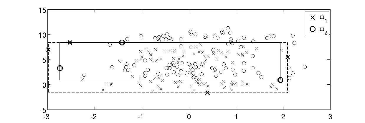
This means that all test observations belonging to and lying outside will be misclassified!
Figure 3 illustrates decision regions built by NCC. The dashed rectangle represents and the solid rectangle represents . The observations used for building these surfaces are plotted in bold. Notice that any observation located outside the boundaries of will be classified as . However, from the data plot, is most probably belonging to if (the lower boundary of ).
This was the motivation behind combining NCC with any other statistical rule. Such a combination will provide the means for learning how to classify future observations located outside the outer surface . We chose the Linear Discriminant Analysis (LDA) for demonstration; however we could have chosen the Quadratic Discriminant Analysis (QDA) or any other discriminant function, hence the name Nested Cavity Discriminant Analysis (NCDA). However, since the aim behind this combination is to be able to classify observations from the tail of the data distribution, we think that LDA or QDA will be quite sufficient.
The proposed classification rule is simple; we train NCC using the data set to learn the geometric structure and build the decision rule . LDA is also trained with to build the decision rule . The final classification rule will be
| (4) |
5 Simulation and Discussion
A simulation study is conducted to compare NCC, NCDA, LDA, and QDA. several simulation parameters should be considered; however, the purpose of the present article is to provide a preliminary simulation study rather than a comprehensive one—refer to Section 6 for future work currently in progress. The data distributions and are assumed to be normals and mixture of normals (with parameters discussed below), dimensionality is chosen to be 2, 4, 8 and 16, and size of the training set, , is chosen to be 10, 20, 40, 80, 160 and 200 (assuming equal training set sizes for the two classes).
We conducted three sets of experiments; in each experiment we train the classifier on a finite training set (of the selected size ), and test on a testing set of size 1000 observations per class to mimic the population. Each training and testing represents one Monte-Carlo (MC) trial. We typically use 1000 MC trials; in each we train on a different training set (of the same size) drawn from the same population and test on the same 1000-observation-per-class testing set.
We measure the performance in terms of error rate . The population parameters of interest, then, are the mean (over the training sets of the same size) performance and the variance . For each experiment we plot the mean and the standard deviation of the performance versus the reciprocal of the training set size.
The first set of experiments assumes and to be multinormal. The mean vector is set to zero vector and the mean vector is set to , where is a vector whose all components are equal to 1 and is a constant that can be used to adjust the classes separability; for our current simulation study we set it to 1. Covariance matrices are set to identity matrix. Figure 4 presents the results of this configuration.
The figure illustrates the typical performance of the LDA and QDA that is well known in the literature; (Chan et al. 1998, e.g., see). The LDA is the winner if compared to the other three, since it is the Bayes classifier for this configuration. However, the NCC behaves the other way around for low dimensionality; its performance deteriorates as the training set size increases! The interpretation of these results is interesting. For simplicity, consider the case of ; the two distributions will look like two circular clouds, one centered at the origin and the other is centered at . With very small training data set, we can imagine that the mean decision surface is a square centered at the origin and enclosed within the first cloud. This will lead to a misclassification for all the testing observations coming from and occur outside the square. Increasing the training set size gives a chance to more training observations to occur at the tail of the distribution. Hence, this will widen the decision surface (the square)—refer to Section 3 for information on how NCC works; this decreases the misclassification rate from the first distribution. Therefore, the performance will increase with the training sample size until the decision surface encloses—roughly speaking—the first cloud, yet, did not intersect with the second cloud. Increasing the training sample size more will allow the decision surface to grow until it intersects with the second cloud, the time at which the second type of error will increase.
The improvement of NCDA over the NCC is evident for all dimensions and for all sample sizes; even, it comes closer to the LDA for higher dimensions.
The second set of experiments assumes to be a mixture of two Gaussians, named and , with identity covariance matrices and mean vectors and respectively. is assumed to be normal with identity covariance matrix and ; we set . This means that is symmetric bimodal and is symmetric and lying between the two bumps of . Figure 5 presents the results of this configuration.
The flat performance of the LDA at 0.5 error rate is not a surprise; this is due to the fact that the problem is symmetric and the hyper plane of symmetry, which will be the decision surface, divides each distribution into two regions each has 0.5 probability. The QDA is the winner for its ability to build quadratic surfaces capable of surrounding observations from . In this configuration the performance of the NCC gets worse as the dimensionality increases. This is in contrast to the results of the first configuration. Moreover, at some training set sizes we get , which means that the NCC rule has to be flipped to produce a mean error rate of . Therefore, the sign of the rule varies with the training set size! and has to be determined by estimating the error rate using one of the resampling techniques, e.g., cross validation. We can also notice that NCDA outperforms NCC universally.
The third set of experiments assumes both and to be a mixture of two Gaussians (with two different mean vectors and same identity covariance matrix). The first mean vector of , , is set to zero vector. The second mean vector of , , is set to . The first mean vector of , , is set to . The second mean vector of , , is set to ; again, we chose . Figure 6 presents the results of this configurations.
From the figure we can observe that NCC, in the majority of experiments, is inferior to the other three classifiers, while the NCDA outperforms all of them in many cases (except at ).
6 Conclusion and future work
In this article we introduced a modification on the NCC classifier by combining it with the LDA; we coined the name NCDA on the new classifier. We established a preliminary simulation study to compare the performance of the NCC and NCDA to two basic classifiers, LDA and QDA. Our simulation study reveals that the NCC is inferior to all other three classifiers almost at all considered dimensions, training sample sizes, and distributions. This is in contrast to what has been reported in some literatures (Inselberg 2002, e.g.,). Our proposed classifier, NCDA, outperforms NCC in all experiments; moreover, it outperforms both LDA and QDA in some experiments.
Our future work, currently under progress in our group, considers several points. First, we are planning for more comprehensive simulation study for more understanding of the behavior of NCC and NCDA. Second, we always advocate for using the Area Under the receiver operating characteristic Curve (AUC) (Hanley and McNeil 1982, see, e.g.,) as a performance measure, since it is independent of the threshold at which we make our decision. However, in the present article, we measure the performance of a classifier in terms of the error rate for two reasons. (1) error rate is the performance measure that was used in Inselberg 2002 to compare the NCC to other classifiers. (2) measuring the performance in terms of the AUC only suits a classifier whose output is given in terms of quantitative scores rather than binary decisions as NCC and NCDA. The work currently under progress in our group is considering converting the NCC, and its smarter version NCDA, to score-based classifiers to allow us to assess them in terms of the AUC (Yousef 2019a; Yousef 2019d; Yousef 2013). In addition, we have the opportunity to apply a whole literature of nonparametric estimation procedures including our methods: estimating uncertainty using influence function (Yousef et al. 2005), estimating uncertainty using UMVU estimation (Yousef et al. 2006; Chen et al. 2012b; Chen et al. 2012a), and estimating uncertainty using cross validation estimators (Yousef 2019c; Yousef 2019b), among others.


References
- Chan et al. (1998) Chan, H.P., Sahiner, B., Wagner, R.F., Petrick, N., 1998. Effects of Sample Size on Classifier Design for Computer-Aided diagnosis. Medical Imaging 1998: Image Processing, Pts 1 and 2 3338, 845–858 1574.
- Chen et al. (2008) Chen, C.h., Härdle, W., Unwin, A., 2008. Handbook of data visualization. Springer, Berlin.
- Chen et al. (2012a) Chen, W., Gallas, B.D., Yousef, W.A., 2012a. Classifier Variability: Accounting for Training and testing. Pattern Recognition 45, 2661–2671. URL: https://doi.org/10.1016/j.patcog.2011.12.024, doi:10.1016/j.patcog.2011.12.024.
- Chen et al. (2012b) Chen, W., Yousef, W.A., Gallas, B.D., Hsu, E.R., Lababidi, S., Tang, R., Pennello, G.A., Symmans, W.F., Pusztai, L., 2012b. Uncertainty Estimation With a Finite Dataset in the Assessment of Classification models. Computational Statistics & Data Analysis 56, 1016–1027. doi:10.1016/j.csda.2011.05.024.
- Efron and Tibshirani (1997) Efron, B., Tibshirani, R., 1997. Improvements on Cross-Validation: the Bootstrap Method. Journal of the American Statistical Association 92, 548–560.
- Hanley and McNeil (1982) Hanley, J.A., McNeil, B.J., 1982. The Meaning and Use of the Area Under a Receiver Operating Characteristic ({ROC}) curve. Radiology 143, 29–36.
- Hastie et al. (2001) Hastie, T., Tibshirani, R., Friedman, J.H., 2001. The elements of statistical learning : data mining, inference, and prediction. Springer, New York.
- Inselberg (2002) Inselberg, A., 2002. Visualization and Data Mining of High-Dimensional data. Chemometrics and Intelligent Laboratory Systems 60, 147.
- Inselberg and Avidan (2000) Inselberg, A., Avidan, T., 2000. Classification and visualization for high-dimensional data. URL: https://doi.org/http://doi.acm.org/10.1145/347090.347170, doi:http://doi.acm.org/10.1145/347090.347170.
- Raudys and Pikelis (1980) Raudys, S., Pikelis, V., 1980. On Dimensionality, Sample Size, Classification Error, and Complexity of Classification Algorithm in Pattern Recognition. Pattern Analysis and Machine Intelligence, IEEE Transactions on PAMI-2, 242–252.
- Yousef (2013) Yousef, W.A., 2013. Assessing Classifiers in Terms of the Partial Area Under the Roc curve. Computational Statistics & Data Analysis 64, 51–70. URL: https://doi.org/10.1016/j.csda.2013.02.032.
- Yousef (2019a) Yousef, W.A., 2019a. AUC: nonparametric estiamtors and their smoothness. arXiv preprint arXiv:1907.12851 .
- Yousef (2019b) Yousef, W.A., 2019b. Estimating the standard error of cross-validation-based estimators of classification rules performance. arXiv preprint arXiv:1908.00325 .
- Yousef (2019c) Yousef, W.A., 2019c. A leisurely look at versions and variants of the cross validation estimator. arXiv preprint arXiv:1907.13413 .
- Yousef (2019d) Yousef, W.A., 2019d. Prudence when assuming normality: an advice for machine learning practitioners. arXiv preprint arXiv:1907.12852 .
- Yousef et al. (2005) Yousef, W.A., Wagner, R.F., Loew, M.H., 2005. Estimating the Uncertainty in the Estimated Mean Area Under the {ROC} Curve of a Classifier. Pattern Recognition Letters 26, 2600–2610.
- Yousef et al. (2006) Yousef, W.A., Wagner, R.F., Loew, M.H., 2006. Assessing Classifiers From Two Independent Data Sets Using {ROC} Analysis: a Nonparametric Approach. Pattern Analysis and Machine Intelligence, IEEE Transactions on 28, 1809–1817.