Quantifying the Total Effect of Edge Interventions in Discrete Multistate Networks
Abstract
Developing efficient computational methods to assess the impact of external interventions on the dynamics of a network model is an important problem in systems biology. This paper focuses on quantifying the global changes that result from the application of an intervention to produce a desired effect, which we define as the total effect of the intervention. The type of mathematical models that we will consider are discrete dynamical systems which include the widely used Boolean networks and their generalizations. The potential interventions can be represented by a set of nodes and edges that can be manipulated to produce a desired effect on the system. We use a class of regulatory rules called nested canalizing functions that frequently appear in published models and were inspired by the concept of canalization in evolutionary biology. In this paper, we provide a polynomial normal form based on the canalizing properties of regulatory functions. Using this polynomial normal form, we give a set of formulas for counting the maximum number of transitions that will change in the state space upon an edge deletion in the wiring diagram. These formulas rely on the canalizing structure of the target function since the number of changed transitions depends on the canalizing layer that includes the input to be deleted. We also present computations on random networks to compare the exact number of changes with the upper bounds provided by our formulas. Finally, we provide statistics on the sharpness of these upper bounds in random networks.
aDepartment of Mathematics, University of Kentucky,
Lexington, KY 40506-0027, USA
bDepartment of Mathematics, California Polytechnic
State University, San Luis Obispo, CA 93407-0403, USA
1 Introduction
Boolean networks (BN) have been proposed as an appropriate framework for modeling the state of cells due to their simplicity and the variety of tools available for model analysis Veliz-Cuba et al. 2010; Zañudo & Albert 2015. However, some complex gene interactions cannot be represented in the Boolean setting and several generalizations of the Boolean approach have been developed Thomas & D’Ari 1990. Multistate models, a generalization of the BN framework, where the genes can attain more than two states have been proposed as appropriate models for capturing complex gene expression patterns, such as consideration of three states (low, medium, and high). We note that while in theory it is possible to develop models where the variables can take on any number of possible states (possibly only restricted by the requirement that it needs to be a power of a prime number so that the domain can have the structure of a finite field), in practical applications this number is typically small – rarely larger than 5.
A Gene Regulatory Network (GRN) is a representation of the intricate relationships among genes, proteins, and other compounds that are responsible for the expression levels of mRNA and proteins. Boolean networks have been successfully used to model and study the properties of GRN Albert & Othmer 2003; Li et al. 2004. In particular, Boolean canalizing rules were introduced by S. Kauffman and collaborators Kauffman et al. 2003; Kauffman et al. 2004 and reflect the concept of canalization in evolutionary biology that Waddington pioneered in 1942 Waddington 1957 – that organisms evolve developmental robustness, producing an invariant phenotype even under genetic or environmental perturbations.
In this article, we study the network-wide effect of an experimental intervention that either prevents a regulation from happening or silences a node. Such intervention is modeled through edge deletion and can be achieved via therapeutic drugs that target a specific gene interaction Choi et al. 2012; Campbell & Albert 2019. In Murrugarra & Dimitrova 2015 we introduced methods for quantifying side effects in Boolean networks. However, many of the more recently published discrete dynamical models include variables that take on more than two states due to the need for capturing mechanisms that are not binary in nature Zañudo, Scaltriti & Albert 2017; Remy et al. 2015; Chifman et al. 2017; Espinosa-Soto et al. 2004; Thieffry & Thomas 1995. Consequently, Boolean nested and partially nested canalizing functions were generalized to multistate Murrugarra & Laubenbacher 2011; Murrugarra & Laubenbacher 2012; Kadelka et al. 2017 which enables the possibility of capturing more complex interactions among the genes in the network. Such functions can be viewed as a discrete dynamical system with a stratified structure which consists of hierarchical layers of variables according to their relative influence over the system dynamics.
The ability to quantify the global changes in the dynamics of the network after an external perturbation has important applications. In the presence of external network modifications where the topology of the network changes but the attractor structure remains unchanged, it is still desirable to quantify the changes in other aspects of the dynamics such as the transient time. For instance, in evolutionary biology to simulate evolution one often evolves an ensemble of networks (by performing mutations, crossover, selection, etc.) for many generations Wagner 1996. At the end of the simulations, one measures the changes in the evolved networks to compare with the features of the original ensemble. In Wagner 1996, after simulated evolution, the evolved networks had similar features to the original ones such as the number of attractors and basin sizes. One feature that had changed is the transient time Wagner 1996. The theoretical tools presented in this paper will be useful to measure global changes even if the attractor structure is preserved after an intervention.
There are several published control methods for Boolean networks such as Stable Motifs Zañudo & Albert 2015, Feedback Vertex Sets Zañudo, Yang & Albert 2017, Minimal Hitting Sets Vera-Licona et al. 2013; Klamt et al. 2006, and several others Qiu et al. 2014; Li et al. 2015; Poret & Boissel 2014; Gates & Rocha 2016; Zañudo, Scaltriti & Albert 2017; Sordo Vieira et al. 2019. While these control methods focus on finding control interventions that satisfy a control objective (e.g., to drive the system into a specific attractor), there are very few studies of the total extent of the consequences of applying a certain control action (beyond satisfying the control objective). This paper contributes methods for measuring the impact of the control actions on the dynamics of multistate networks. The type of theoretical tools presented here can help to discriminate control actions with minimal effect on the state space. That is, even if we have different control candidates that can achieve a certain objective, they might have different impact on the dynamics of the network and we might be interested in distinguishing the control action that produces the least changes in the dynamics of the network.
The rest of the paper is structured as follows. In Section 2, we introduce discrete dynamical systems and their representation as polynomial dynamical systems. In Section 3 we define the control actions for multistate networks. In Section 4 we provide a polynomial normal form for discrete functions and then we use this representation to derive a set of formulas for counting the maximum number of transitions in the state space upon edge deletions. In Section 5 we present computational results for random networks. Finally, in Section 6, we provide the conclusions of the paper.
2 Background
A discrete dynamical system can be defined as a dynamical system that is discrete in time as well as in variable states. More formally, consider a collection of variables, each of which can take on values in finite sets . Let be their Cartesian product. A discrete dynamical system in the variables is a function
where each coordinate function is a discrete function on a subset of which represents how the future value of the -th variable depends on the present values of the variables. If , then each is a Boolean rule and is a Boolean network.
In this article, for the purpose of exploiting the algebraic properties of discrete functions, it is assumed that the variables take on values from a finite field . Then using the fact that any discrete function can be represented as a polynomial in , that is , the discrete network can be represented as where each . If any of the variables take on values from a set that cannot be directly identified with a finite field, then it is straightforward to embed the system into a system , where , while preserving the attractor structure of ; see Veliz-Cuba et al. 2010.
Given a discrete network , a directed graph on nodes is associated to as follows: there is a directed edge in from to if appears in , i.e. is in the support of , written . In the context of a molecular network model, this graph represents the wiring diagram of the network.
The dynamics of a discrete network is given by the difference equation ; that is, the dynamics is generated by iteration of . More precisely, the dynamics of is represented by the state space graph , defined as the graph with vertices in which has an edge from to if and only if . In this context, the problem of finding the states where the system will get stabilized is of particular importance. The collection of these special points of the state space are called attractors of a discrete network and elements of the attractors may include steady states (fixed points), where , or cycles, where for some integer . Attractors in network modeling might represent cell types Kauffman 1969 or cellular states such as apoptosis, proliferation, or cell senescence Huang 1999; Shmulevich & Dougherty 2010.
3 Methods
Network interventions can be modeled through edge and node manipulations and can be achieved via therapeutic drugs that target a specific gene interaction Choi et al. 2012; Campbell & Albert 2019. In Murrugarra & Dimitrova 2015; Murrugarra et al. 2016 we provided definitions for these actions in Boolean networks. These definitions are usually used for encoding the control parameters with the purpose of identifying control targets as shown in Murrugarra et al. 2016. In this paper we will consider the deletion and constant expression of edges in the multistate setting.
Throughout the paper, will be a subset of and will be the indicator functions of . That is, they return 1 when is in the set and 0 when is not. The index indicates the node from which the edge begins and the second index is used when necessary to mark the function under consideration.
3.1 Edge Control in Multistate Networks
In the Boolean setting, the deletion of an edge was implemented by setting an input to zero so that the interaction of that input (represented by an edge) was being silenced. For the multistate case, the silencing of the interaction will be applied whenever the control variable is within a range of values of the possible discrete values.
Definition 3.1 (Edge Deletion).
Consider the edge in a wiring diagram. For , the control of the edge consists of manipulating the input variable for in the following way:
For each value of we have the following control settings:
- •
For ,
That is, the control is active and the action represents the removal of the edge .
- •
For ,
That is, the control is not active.
We will also consider the constant expression of edges, which we define as follows.
Definition 3.2 (Constant expression).
Consider the edge in a wiring diagram and . For , the control of the edge consists of manipulating the input variable for in the following way:
For each value of we have the following settings:
- •
For ,
That is, the control is active and the action represents the constant expression (to ) of the edge .
- •
For ,
That is, the control is not active.
Remark 3.3.
Node control of can be defined as setting the function to a constant .
4 Results
In this section we present a definition of -canalizing functions for the multistate case and then we characterize this functions in terms of layers of canalizations. Subsequently, we use this canalizing layers representation to derive an upper bound for the number of changes in the state space of a discrete system upon an edge deletion in the wiring diagram.
4.1 Multistate -Canalizing Functions
In the following definition, we assume that is a permutation on .
Definition 4.1.
The function is a -canalizing function in the variable order with canalizing input sets and canalizing output values if it can be represented in the form
| (1) |
where is a multistate function on variables. When is not a canalizing function, the integer is the canalizing depth of . If is not a constant function, then is called the core function of and is denoted by .
Remark 4.2.
Example 4.3.
Let and . Consider the function
For this function is canalizing (with ) because . However, is not a -canalizing function because . Thus, even though is canalizing for , the function has no layers of canalization. Thus, .
4.2 Layers of canalization in multistate networks
In Theorem 4.4 we provide a polynomial normal description of discrete functions. Basically, this theorem gives a partition of the inputs of the function into canalizing and non-canalizing variables and, within the canalizing ones, we categorize the input variables into layers of canalization. This theorem is a generalization of a theorem in He & Macauley 2016 from Boolean to the multistate case.
Let be a subset of and be the indicator function of the complement of . That is,
Theorem 4.4.
Every multistate function can be uniquely written as
| (2) |
where , is the canalizing depth, is a polynomial that has no canalizing variables, , and . Each variable appears in exactly one of the .
Proof.
If is non-canalizing, then . If is canalizing, then we proceed by induction. For , if is canalizing in but not -canalizing in , then we set . If is -canalizing in , then it can be written as for some set . Then has the form of Equation 2 by setting and . For , if is not -canalizing on any of its variables, then we set . If is -canalizing on , then can be written as for some . Then has the form of Equation 2 by setting . Now assume that Equation 2 is true for any canalizing function that is essential in at most variables (that is, for all functions that depend in at most variables). Let be a function that is essential in variables. If is not -canalizing on any of its variables, then we set . If is -canalizing in , then , where is the product of indicator functions of the complements of sets and has variables. If has no canalizing variables, then has the form of Equation 2 with . If is canalizing, then by the inductive hypothesis can be written as
Thus, has the form of Equation 2. ∎
Remark 4.5.
For a multistate nested canalizing function, the formula in Equation 2 reduces to
| (3) |
as was shown in Kadelka et al. 2017.
In the following example we describe a -canalizing function with noncanalizing variables.
Example 4.6.
4.3 Upper bounds
Using the polynomial normal form of multistate functions in Theorem 4.4, we derive a set of formulas for counting the maximum number of transitions that will change in the state space upon an edge deletion in the wiring diagram. The formulas presented here are generalizations from the Boolean case to the multistate setting of the formulas we presented in Murrugarra & Dimitrova 2015.
For the next theorem, we are going to assume that the functions of the discrete network are written in the format of Theorem 4.4. That is, for the coordinate function has the following form,
| (4) |
where , is the canalizing depth, is a polynomial with no canalizing variables, , and . Each variable appears in exactly one of .
Remark 4.7.
Note that the function has layers and there are variables in each layer for .
In the following theorem, we assume that the canalizing input sets are all of the same size for all the variables. In Theorem 4.10 we study the general case where the canalizing input sets of the variables can be different.
Theorem 4.8.
Let be a multistate network where is a -canalizing function written as in Eq. 4 with the numbers of variables in layers , respectively. Let be in the layer, where and is the number of layers. Suppose that all canalizing variables have the same canalizing input set and that . Then, the maximum number of transitions in the state space that will change upon deletion of is given by
| (5) |
Proof.
Let . The number of input vectors where the other canalizing variables (not ) of do not take on their canalizing input is . For these input vectors, if was already set to 0 or to any other of its canalizing values in , then the output of will not change as a result of deleting . Finally, since we have non-canalizing variables, the total number of input vectors for which the output of can possibly change is . ∎
Remark 4.9.
Theorem 4.10.
Let be a multistate network where is a -canalizing function written as in Eq. 4 with the numbers of variables in layers , respectively. Let be in the layer, and is the number of layers. The maximum number of transitions in the state space that will change upon deletion of is given by
| (6) |
where
Proof.
The strategy is to first count the number of inputs that do not contain values from the canalizing sets of the variables in the first layers (that do not contain ). Thus, the term in the first line of Equation 7 counts the number of non-canalizing inputs in the previous layers to the layer containing ; the term inside the second set of parentheses of Equation 7 counts the number of non-canalizing inputs of the variables (except of ) in the layer containing ; the last term in Equation 7 counts the number of non-canalizing inputs of . For the last term, notice that deleting results in setting in . If 0 is in the canalizing set of , , then the rest of the values in will yield the same output as 0. Since of the input values in the transition table of contain a canalizing value for , it is the remaining of the table that can potentially change as a result of the edge deletion. On the other hand, if , then it is the inputs not in that have the potential to change the output as a result of deleting which constitutes of the transition table, with of the table that can potentially change as a result of the edge deletion. Thus, to obtain Equation 6 we multiply the following expressions:
| (7) |
∎
Remark 4.11.
Proposition 4.12.
Let be a multistate network where is written as in Equation 4. Let . The maximum number of transitions in the state space that will change upon deletion of is
| (8) |
Remark 4.13.
- 1.
This upper bound is sharp.
- 2.
When , the expression reduces to , where is the canalizing depth.
- 3.
If has no canalizing variables, then the formula in Equation 8 reduces to .
Proposition 4.14.
Let be a multistate network where is written as in Equation 4. If is canalizing but not -canalizing with canalizing variable and input set , then there are two cases to consider:
- 1.
The deletion of will result in up to
(9) transitions, where
- 2.
Let that is not canalizing. Then the maximum number of transitions in the state space that will change upon deletion of is
(10)
Remark 4.15.
- 1.
This upper bound is sharp.
- 2.
If has more than one canalizing variables (but it is still not 1-canalizing), then the formula in Equation 10 becomes
(11) where each is a canalizing variable and is the number of canalizing variables of .

5 Applications
To provide further insights into the results presented above and to illustrate the use of the formulas here we present numerical results for random networks where we compare the exact number of changes to the upper bounds provided by the formulas.
For the next examples, we generated random networks with scale-free structure using the Barabasi-Albert algorithm Barabasi & Albert 1999. We note that the Barabasi-Albert algorithm produces undirected edges but for our examples we need directed edges. Thus, for each undirected edge between and , we converted the edge into either or at random.
Example 5.1 (Boolean Case).
In order to calculate the exact number of changes we use random networks with 10 nodes. For each network, we selected the node with the maximum in-degree and generated a random partition of its inputs to assign the canalizing layers. The functions of the other nodes were generated at random.
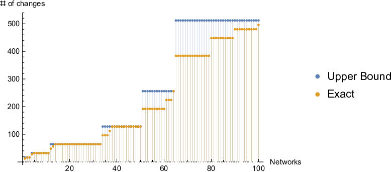
In Figure 1 we show statistics for the number of changes in the first layer. The average maximum in-degree for the networks in Figure 1 is (). The average number of variables in the first layer is (). The average number of changes in the first layer is () and the average upper bound is ().
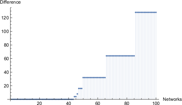
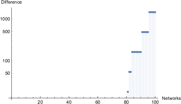
In Figure 2 we present statistics of the number of changes as well the difference between the exact number of changes and the upper bound provided by the formulas. For these networks, in about 40% of the cases the upper bounds match the exact number of changes.
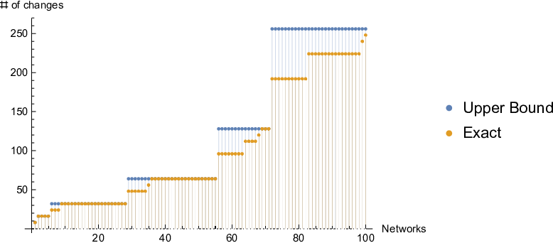
In Figure 3 we show statistics for the number of changes in the second layer. The average maximum in-degree for the networks in Figure 3 is (). The average number of variables in the first layer is (). The average number of variables in the second layer is (). The average number of changes in the second layer is () and the average upper bound is ().
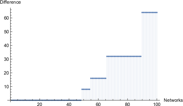
In Figure 4 we present statistics of the number of changes as well the difference between the exact number of changes and the upper bound provided by the formulas. For these networks, in about 50% of the cases the upper bounds match the exact number of changes.

Example 5.2 (Multistate Case).
Here we also use random networks with scale-free structure with and nodes. For each network, we selected the node with the maximum in-degree and generated a random partition of its inputs to assign the canalizing layers. The functions of the other nodes were generated at random.
In Figure 5 we show statistics for the number of changes in the first layer. The average maximum in-degree for the networks in Figure 5 is (). The average number of variables in the first layer is (). The average number of changes in the first layer is () and the average upper bound is ().
In Figure 6 we present statistics of the difference between the upper bounds provided by the formulas and the exact number of changes. For these networks, in about 75% of the cases the upper bounds match the exact number of changes.
In Figure 7 we show statistics for the number of changes in the second layer. The average maximum in-degree for the networks in Figure 7 is (). The average number of variables in the first layer is (). The average number of variables in the second layer is (). The average number of changes in the second layer is () and the average upper bound is ().

In Figure 8 we present statistics of the difference between the the upper bound provided by the formulas and the exact number of changes. For these networks, in about 80% of the cases the upper bounds match the exact number of changes.
6 Conclusions
In this paper we present practical methods for quantifying the global changes that result from an application of an external intervention in the network, which we called the total effect of the intervention. We emphasized that, while there are several methods for identifying control targets in discrete networks, there have been very few studies focusing on the total extent of the consequences of applying a certain control action (beyond satisfying the control objective). This paper contributes methods for measuring the number of changed transitions in the state space upon the application of an edge control in multistate networks. The approach is based on a polynomial normal form description of discrete functions that provides a way of categorizing the inputs of the function and therefore of quantifying their impact on the dynamics of the network. The main computational cost of our approach is in obtaining the canalizing layers format of the functions which we used to derive our formulas. Once the functions are written in the layers format, it is straightforward to apply the formulas to calculate the upper bound. We note that obtaining the layers format could be a formidable task with exponential complexity on the number of inputs in the worst case but for the type of networks we are studying (i.e. biological networks) we believe that our approach is still practical. We applied our methods to randomly generated multistate models and verified that in many cases the upper bounds provided by our formulas were accurate. We also observed that the upper bounds tend to be more accurate when the edge interventions happen in a less dominant layer.
References
- (1)
- Albert & Othmer (2003) Albert, R. & Othmer, H. G. (2003), ‘The topology of the regulatory interactions predicts the expression pattern of the segment polarity genes in drosophila melanogaster’, J Theor Biol 223(1), 1–18.
- Barabasi & Albert (1999) Barabasi & Albert (1999), ‘Emergence of scaling in random networks’, Science 286(5439), 509–12.
- Campbell & Albert (2019) Campbell, C. & Albert, R. (2019), ‘Edgetic perturbations to eliminate fixed-point attractors in boolean regulatory networks’, Chaos 29(2), 023130.
- Chifman et al. (2017) Chifman, J., Arat, S., Deng, Z., Lemler, E., Pino, J. C., Harris, L. A., Kochen, M. A., Lopez, C. F., Akman, S. A., Torti, F. M., Torti, S. V. & Laubenbacher, R. (2017), ‘Activated oncogenic pathway modifies iron network in breast epithelial cells: A dynamic modeling perspective’, PLoS Comput Biol 13(2), e1005352.
- Choi et al. (2012) Choi, M., Shi, J., Jung, S. H., Chen, X. & Cho, K.-H. (2012), ‘Attractor landscape analysis reveals feedback loops in the p53 network that control the cellular response to dna damage’, Sci. Signal. 5(251), ra83.
- Espinosa-Soto et al. (2004) Espinosa-Soto, C., Padilla-Longoria, P. & Alvarez-Buylla, E. R. (2004), ‘A gene regulatory network model for cell-fate determination during arabidopsis thaliana flower development that is robust and recovers experimental gene expression profiles’, Plant Cell 16(11), 2923–39.
- Gates & Rocha (2016) Gates, A. J. & Rocha, L. M. (2016), ‘Control of complex networks requires both structure and dynamics’, Scientific reports 6, 24456.
- He & Macauley (2016) He, Q. & Macauley, M. (2016), ‘Stratification and enumeration of boolean functions by canalizing depth’, Physica D: Nonlinear Phenomena 314, 1–8.
- Huang (1999) Huang, S. (1999), ‘Gene expression profiling, genetic networks, and cellular states: an integrating concept for tumorigenesis and drug discovery’, J Mol Med (Berl) 77(6), 469–80.
- Kadelka et al. (2017) Kadelka, C., Li, Y., Kuipers, J., Adeyeye, J. O. & Laubenbacher, R. (2017), ‘Multistate nested canalizing functions and their networks’, Theoretical Computer Science 675, 1–14.
- Kauffman (1969) Kauffman, S. A. (1969), ‘Metabolic stability and epigenesis in randomly constructed genetic nets’, J Theor Biol 22(3), 437–67.
- Kauffman et al. (2003) Kauffman, S., Peterson, C., Samuelsson, B. & Troein, C. (2003), ‘Random boolean network models and the yeast transcriptional network’, Proceedings of the National Academy of Sciences 100(25), 14796–14799.
- Kauffman et al. (2004) Kauffman, S., Peterson, C., Samuelsson, B. & Troein, C. (2004), ‘Genetic networks with canalyzing boolean rules are always stable’, Proc Natl Acad Sci U S A 101(49), 17102–7.
- Klamt et al. (2006) Klamt, S., Saez-Rodriguez, J., Lindquist, J. A., Simeoni, L. & Gilles, E. D. (2006), ‘A methodology for the structural and functional analysis of signaling and regulatory networks’, BMC Bioinformatics 7, 56.
- Li et al. (2004) Li, F., Long, T., Lu, Y., Ouyang, Q. & Tang, C. (2004), ‘The yeast cell-cycle network is robustly designed’, Proc Natl Acad Sci U S A 101(14), 4781–6.
- Li et al. (2015) Li, R., Yang, M. & Chu, T. (2015), ‘Controllability and observability of boolean networks arising from biology’, Chaos 25(2), 023104.
- Murrugarra & Dimitrova (2015) Murrugarra, D. & Dimitrova, E. S. (2015), ‘Molecular network control through boolean canalization’, EURASIP J Bioinform Syst Biol 2015(1), 9.
- Murrugarra & Laubenbacher (2011) Murrugarra, D. & Laubenbacher, R. (2011), ‘Regulatory patterns in molecular interaction networks’, Journal of Theoretical Biology 288(0), 66–72.
- Murrugarra & Laubenbacher (2012) Murrugarra, D. & Laubenbacher, R. (2012), ‘The number of multistate nested canalyzing functions’, Physica D: Nonlinear Phenomena 241(10), 929–938.
- Murrugarra et al. (2016) Murrugarra, D., Veliz-Cuba, A., Aguilar, B. & Laubenbacher, R. (2016), ‘Identification of control targets in boolean molecular network models via computational algebra’, BMC Syst Biol 10(1), 94.
- Poret & Boissel (2014) Poret, A. & Boissel, J.-P. (2014), ‘An in silico target identification using boolean network attractors: Avoiding pathological phenotypes’, Comptes rendus biologies 337(12), 661—678.
- Qiu et al. (2014) Qiu, Y., Tamura, T., Ching, W.-K. & Akutsu, T. (2014), ‘On control of singleton attractors in multiple boolean networks: integer programming-based method’, BMC Syst Biol 8 Suppl 1, S7.
- Remy et al. (2015) Remy, E., Rebouissou, S., Chaouiya, C., Zinovyev, A., Radvanyi, F. & Calzone, L. (2015), ‘A modeling approach to explain mutually exclusive and co-occurring genetic alterations in bladder tumorigenesis’, Cancer Research 75(19), 4042–4052.
- Shmulevich & Dougherty (2010) Shmulevich, I. & Dougherty, E. R. (2010), Probabilistic Boolean Networks - The Modeling and Control of Gene Regulatory Networks, SIAM.
- Sordo Vieira et al. (2019) Sordo Vieira, L., Laubenbacher, R. C. & Murrugarra, D. (2019), ‘Control of intracellular molecular networks using algebraic methods’, Bull Math Biol 82(1), 2.
- Thieffry & Thomas (1995) Thieffry, D. & Thomas, R. (1995), ‘Dynamical behaviour of biological regulatory networks–ii. immunity control in bacteriophage lambda’, Bull Math Biol 57(2), 277–97.
- Thomas & D’Ari (1990) Thomas, R. & D’Ari, R. (1990), Biological feedback, CRC Press, Boca Raton.
- Veliz-Cuba et al. (2010) Veliz-Cuba, A., Jarrah, A. S. & Laubenbacher, R. (2010), ‘Polynomial algebra of discrete models in systems biology’, Bioinformatics 26(13), 1637–43.
- Vera-Licona et al. (2013) Vera-Licona, P., Bonnet, E., Barillot, E. & Zinovyev, A. (2013), ‘Ocsana: optimal combinations of interventions from network analysis’, Bioinformatics 29(12), 1571–3.
- Waddington (1957) Waddington, C. H. (1957), The strategy of the genes: a discussion of some aspects of theoretical biology, Allen & Unwin, London.
- Wagner (1996) Wagner, A. (1996), ‘Does evolutionary plasticity evolve?’, Evolution 50(3), 1008–1023.
- Zañudo & Albert (2015) Zañudo, J. G. T. & Albert, R. (2015), ‘Cell fate reprogramming by control of intracellular network dynamics’, PLoS Comput Biol 11(4), e1004193.
- Zañudo, Scaltriti & Albert (2017) Zañudo, J. G. T., Scaltriti, M. & Albert, R. (2017), ‘A network modeling approach to elucidate drug resistance mechanisms and predict combinatorial drug treatments in breast cancer’, Cancer convergence 1(1), 5.
- Zañudo, Yang & Albert (2017) Zañudo, J. G. T., Yang, G. & Albert, R. (2017), ‘Structure-based control of complex networks with nonlinear dynamics’, Proc Natl Acad Sci U S A 114(28), 7234–7239.