Control-Theoretic Models of Environmental CrimeThanks: Submitted to the editors June 24th, 2019.
Abstract
We present two models of perpetrators’ decision-making in extracting resources from a protected area. It is assumed that the authorities conduct surveillance to counter the extraction activities, and that perpetrators choose their post-extraction paths to balance the time/hardship of travel against the expected losses from a possible detection. In our first model, the authorities are assumed to use ground patrols and the protected resources are confiscated as soon as the extractor is observed with them. The perpetrators’ path-planning is modeled using the optimal control of randomly-terminated process. In our second model, the authorities use aerial patrols, with the apprehension of perpetrators and confiscation of resources delayed until their exit from the protected area. In this case the path-planning is based on multi-objective dynamic programming. Our efficient numerical methods are illustrated on several examples with complicated geometry and terrain of protected areas, non-uniform distribution of protected resources, and spatially non-uniform detection rates due to aerial or ground patrols.
keywords
Optimal Control, Hamilton-Jacobi, Multiobjective Path-Planning, Randomly-Terminated Processes, Environmental Crime.Funding.
This work is supported in part by the National Science Foundation grant DMS-1738010. The second author’s work is also supported by the Simons Foundation Fellowship.AMS
49N90, 90C29, 35F21, 65N06, 91B76Section 1 Introduction
Mathematical modeling of environmental crimes in national parks has been a growing area of research. Both the authorities and non-governmental conservation organizations strive to prevent illegal extraction activities, including wildlife poaching and illegal logging. In 2010, Albers [1] introduced a framework where the government chooses a patrol density (determining the probability of detection at each location) in such a way as to maximize the pristine area of the park. The perpetrators then choose where to extract resources in such a way as to maximize their expected payoff. The problem of choosing patrol densities to maximize the pristine area has also been explored in [23]. In recent years, patrol strategies based on graph-theoretic models (such as PAWS [19] and INTERCEPT [25]) have even been deployed in actual national parks.
The original Albers model [1] was posed with many restrictive/unrealistic assumptions, including the radial symmetry of the protected area, patrol strategies, and resource distribution. In a recent paper by D.J. Arnold et al [4], these restrictions were largely removed, with numerical simulations on arbitrary two-dimensional domains and the terrain directly affecting the speed of perpetrators. The key mathematical tool employed in [4] is the level-set method, developed to track the propagation of interfaces by solving time-dependent Hamilton-Jacobi PDEs [29]. We begin by briefly reviewing both of these models in Section 2.
In this paper, we offer a significantly different perspective on how to generalize the Albers model to arbitrary domains. As explained in Section 3, our main focus is on a careful treatment of the path-planning problem faced by the extractors. Capturing their rational behavior yields a more accurate prediction of affected areas and allows for a better planning of optimal patrol strategies. We show that the perpetrators optimization problem changes significantly based on the consequences of being spotted while transporting the protected resources.
In our first “Model G”, where authorities use “ground patrols” to spot the extractors, any detection leads to an immediate confiscation, with perpetrators subsequently switching to the fastest path to leave the protected area. The probability of being detected along any originally chosen path is not a sufficient description here, since it does not reflect the expected duration of that post-confiscation trip. We handle this challenge by finding the optimal controls for a suitable randomly-terminated process. In our second “Model A”, where authorities run “aerial patrols,” it is assumed that the perpetrators remain oblivious of when a detection happens and are only apprehended later, once they reach the boundary of the protected area. As a result, they always use their pre-selected trajectories, which are chosen to balance the probability of detection against the time or (cumulative difficulty) of the post-extraction trip. In standard path-planning applications, the goal is usually to minimize the integral of some “running cost” along a chosen trajectory. The key difficulty of this second model is that no such running cost can be explicitly defined to recover trajectories maximizing the extractor’s expected profit. Nevertheless, in section 4 we show that this problem can be solved using the tools of multi-objective optimal control theory.
We discuss efficient numerical methods for the associated stationary Hamilton-Jacobi-Bellman PDEs in Section 5. Our algorithms are illustrated on a number of examples in Section 6, including on realistic terrain maps from Yosemite National Park in California and Kangaroo Island in South Australia. We show that Models A and G often yield very different perpetrator trajectories and also differ in their predictions of the subdomain unaffected by extraction activities. We conclude by discussing possible extensions and directions for future work in section 7.
Section 2 Prior Work
The model proposed by Albers in [1] is based on a one-period Stackelberg game between the protected area managers (PAMs) and the extractors targeting a protected domain PAMs decide on their patrol strategy, defining the pointwise rate of extractor-detection and respecting the known budget constraints for patrolling efforts:
| (1) |
with a constant modeling a possible increase in marginal costs of maintaining a higher detection rate.
Once is chosen, it becomes known to extractors, who select which parts of to target, trying to maximize their expected profit (defined below). Correspondingly, PAMs’ goal is to select that will minimize the impact of the extractors’ best/rational response. This can be interpreted as either maximizing the “pristine” area unaffected by the extractors or maximizing the amount of non-extracted resources. In Albers’ original model both of these interpretations are equivalent since she assumes a homogeneous distribution of protected resources.
Even more restrictively, the domain is assumed to be a unit disk, with extractors evenly distributed along its boundary. This radial symmetry dramatically simplifies the problem and allows for analytical solutions for the optimal behavior of all participants. E.g., it is easy to see that only radially symmetric would need to be considered – Albers further restricts this to piecewise-constant radial functions, with positive rate of detection in an annulus between radial distances and from and everywhere else. The same radial symmetry ensures that extractors travel along straight lines from toward the center of and their entire strategy can be encoded by the chosen depth of penetration Albers assumes that extractors travel to their chosen location unimpeded (since they have not broken any law yet), then turn around and start extracting resources as they retrace their steps to . If they are detected by PAMs on their way back, the extracted resources are confiscated and they have to return to empty-handed, incurring the time/opportunity cost without any reward. Thus, each extractor chooses to maximize their expected profit
| (2) |
where and are respectively the cumulative probability of being detected, the value of extracted resources, and the cost of traversing the path – all corresponding to going distance into before starting to extract resources. While this is not explicitly specified in [1], can also include the cost of getting to the point from which the extraction starts. A more subtle point is that includes the value of all resources extracted along the way back. In the general setting, this continuous-along-the-path extraction would induce a competition among the extractors searching for the best paths through , but the radial symmetry mitigates this effect. However, this makes it harder to justify the one-period nature of the model: as the extractors’ actions deplete the resources in parts of the protected area, that would obviously change the future optimizations problems (faced by both PAMs and the extractors) even in a radially symmetric setting. Such dynamic consequences of “incomplete enforcement” are acknowledged in [1] and also well-known in practice; e.g., [32, 31].
A recent paper by D.J. Arnold et al in [4] extended the above general approach to more realistic protected areas. Their model allows for general domain geometries, resource distributions, terrain effects, and PAMs’ strategies. One important distinction is that, unlike Albers, they model the extraction as occurring at isolated points. An advantage of this approach is that this reduces competition among the extractors (since the paths-to- traversed by others don’t affect the value of what you are currently trying to extract). For an extractor targeting a location they define the expected profit as
| (3) |
where is the value of resources available for extraction in a small neighborhood of , while is the effective cost of a post-extraction trajectory, accounting both for the time/difficulty of travel from to and for the expected losses from a possible capture. A perpetrator chooses this trajectory to minimize (and thus maximize ). In [4] this optimization is performed implicitly by using a level set method originally developed for tracking the propagation of interfaces [29]. The authors show that, in an Albers-style radially symmetric setting with unit walking speed of perpetrators, their approach produces the same as predicted by formula (2). A comparison with (3) thus suggests an explicit interpretation
For any chosen constant Arnold et al compute simultaneously for all extraction positions such that The idea is to find equal-effective-cost curves by using the level sets of an auxiliary time-dependent function satisfying a Hamilton-Jacobi PDE
| (4) |
with initial conditions distance from to Assuming that is some interface starting from and monotonically advancing into with the normal speed , its evolution is encoded by the zeroth level-set of solving the above PDE; i.e., For the purposes of this model, the authors choose their normal speed of the interface to be
| (5) |
where is the extractor’s local speed of motion defined by the terrain at , and a parameter encodes the degree of extractor’s risk-aversion. This formula is motivated phenomenologically: represents the extractor’s “slowness of motion” and represents his expected losses (per unit time, while traveling through ). An increase in either of these terms should make the effective cost higher. Once is computed, the authors define implicitly through
with an optimal path to from any such recovered via gradient descent in . The process is then repeated for multiple values of until (and thus also ) are defined for all gridpoints of some grid imposed on
In another departure from Albers’ original model, the authors assume that extractors will target all locations where is within factor from its maximal value; i.e., the extraction happens on the set
(One drawback of this assumption is that extraction will always happen on some part of , regardless of how high the detection rate might be.) The authors then define the pristine area by excluding not only the above but also the union of narrow corridors around optimal trajectories from . The latter are approximated by starting from a finite number of points selected uniformly at random in . Since there is no extraction along the path, the motivation for this exclusion might perhaps be based on extraction-unrelated damage to the protected area. While [4] does not present a systematic method for optimizing PAMs’ choice of , the authors use the above interpretation to compare the effectiveness of several (ad hoc) patrol strategies staying within the specified patrol budget. Their simulations (using and ) are based on the terrain data from Yosemite National Park in California and Kangaroo Island in South Australia, which they have also kindly shared with us to conduct the numerical experiments presented in section 6.
We end this section by discussing the difference between path planning to avoid detection vs capture/interception. Even if the former always leads to the latter, there is still a very subtle modeling question of whether the capture happens immediately upon detection and, if there is a significant delay, whether the extractors learn that they have been detected before the capture. These issues are not important in [1] since the extractors’ paths are always radial in Albers’ setting. But Arnold et al describe path-planning that strikes a balance between the time of travel and risk of detection all the way to the boundary – with no provision for switching to quicker/easier paths if authorities manage to intercept the extractors en route and confiscate their haul. Thus, we believe that the model in [4] is more suitable for the setting where the extractors remain oblivious of their detection (perhaps in the case of aerial surveillance) and are only intercepted upon reaching .
Section 3 Extractor’s path-planning
This section defines the optimization problem faced by a perpetrator
deciding whether to extract resources from a fixed location .
As in [4], our approach is based on “pointwise” extraction decisions, but since these resources are typically continuously distributed in the protected area this requires further clarification. We will consider a fine grid of possible extraction sites, with each representing a center of its extraction cell and representing the value of all resources that can be extracted from
that cell.
The same grid will be also used to solve the PDEs numerically in section 5.
We will further assume that
- 1.
The extractor can enter through any part of and has no reason to avoid surveillance from PAMs until he reaches the extraction site
- 2.
While traveling through , the extractor may freely choose any measurable “control function” specifying his chosen direction of motion for all times . This defines the corresponding trajectory since his (isotropic) speed of motion reflects the local terrain and is a part of the input data.
- 3.
The time/difficulty cost of traveling through is reflected by integrating some known running cost along his chosen trajectory. One natural choice is reflecting the monetary value the extractor associates with each hour of his time spent on a trip. (To normalize the units, all of our numerical examples use for all pre-extraction and post-extraction travel through ) But a non-constant can be also used to reflect the extractor’s distaste for some parts of the protected area (e.g., due to vegetation).
- 4.
Once he reaches , the extraction in is instantaneous and the extractor immediately starts along his (possibly different) path to the boundary.
- 5.
On the way back to , he is trying to minimize both the time/cost of travel and the probability of being spotted by PAMs through aerial surveillance.
- 6.
The extractor has full prior knowledge of PAMs’ location-dependent detection rate
- 7.
Rational extractors will target all sites for which the expected profit of their optimal roundtrip is above some threshold level . This leaves a pristine area
(Our numerical experiments use ) Note that this is different from the approach in [4] not only in providing an absolute threshold, but also because we don’t exclude from any corridors around post-extraction trajectories. We believe that this is more consistent with the notion of localized extractions.
Computing the expected profit requires solving two different optimization problems: (a) finding the best (PAMs-ignoring) pre-extraction trajectory from to and then (b) finding the best post-extraction trajectory from to , balancing the cost of travel and risk of detection. We will start by addressing (a) in section 3.1 since it is easy to solve by standard tools of single-criterion deterministic optimal control theory. Below we provide only a very brief introduction, referring to standard references (e.g., [10] and [5]) for technical details.
We will then use two models to address (b) under very different assumptions about the nature of PAMs’ enforcement activities and the information available to perpetrators:
Model G (ground patrols):
If the extractor is detected while traveling with protected resources, he is immediately apprehended and the resources are confiscated. From there on, the perpetrator does not attempt extracting anything on this trip and simply seeks to minimize the integral of on his way to
Model A (aerial patrols):
The extractor has no way of learning if or when the detection occurs. But if it happens, he is later apprehended with probability one upon reaching and his entire haul is confiscated.
We will show that these two interpretation require fairly different mathematical tools: Model G is best recast as an optimal control of a randomly-terminated process (subsection 3.2), while Model A requires the techniques from multi-objective dynamic programming (subsection 3.3). The numerical methods for both versions are covered in section 5.
Subsection 3.1 Getting to the extraction point
We will use to denote the cost of the optimal pre-extraction trajectory from to . But to make the discussion closer to the canonical optimal control setting, we will reverse the direction of the trajectory in (a), looking instead for a -optimal way to reach from . (Based on our isotropy assumptions, this direction reversal will change neither the time of travel nor the integral of along any considered trajectory.) The added benefit is that the same discussion will be a useful starting point for solving (b).
The extractor’s time-dependent position in the domain will be specified by
| (6) |
Once is chosen, this defines the exit time and the cumulative cost of starting at and using
If the extractor only cares about selecting a path to minimize this it is easy to accomplish by traditional tools of single-criterion dynamic programming introduced by Richard Bellman in the 1950s.
The value function is defined as the minimum cost one has to pay starting from ; i.e., A Taylor series expansion along the optimal trajectory can be used to derive a Hamilton-Jacobi-Bellman (HJB) PDE that must satisfy if it is sufficiently smooth. For our isotropic cost and dynamics, this PDE is merely an Eikonal equation
| (7) |
solved with Dirichlet boundary conditions on . Unfortunately, in general (7) does not have a classical/smooth solution, and there are infinitely many weak (Lipschitz-continuous) solutions. Additional test conditions were introduced by Crandall and Lions [15] to select among them the unique viscosity solution coinciding with the value function of the above control problem. Several highly efficient methods for solving Eikonal PDEs numerically were developed in the past 25 years; see a brief overview at the end of section 5.
We note that taking results in So, both the distance-from-boundary and the min-time-from-boundary can be also found by solving the Eikonal equations and with zero boundary conditions. If , then the minimum cost of reaching from is simply
The characteristic curves of HJB equations are the optimal trajectories, which in the Eikonal case coincide with the gradient lines of the viscosity solution. I.e., once the value function is computed, an optimal trajectory can be found via gradient descent in . Since this function is differentiable almost everywhere, the optimal trajectories are unique for almost all
Remark 1.
We note that the function used in [4] can also be found directly (without using a level-set formulation) by solving an Eikonal equation While the level set method is a much more general interface tracking approach, the fast Eikonal solvers are likely to be more efficient for the current application.
Subsection 3.2 Returning with the loot (Model G: ground patrols)
Here we assume that a detection leads to an immediate apprehension and confiscation of extracted resources. Thus, it is natural to split the post-extraction trajectory into two parts: a pre-detection trajectory (leading all the way to if the detection was avoided) and a post-detection trajectory (chosen by a perpetrator to simply minimize the integral of up to after the confiscation). Suppose the perpetrator starts from an extraction point and manages to reach some undetected. From there on, he uses a control moving from along a trajectory with a possible detection at some time before reaching the boundary. His remaining cost is
Of course, the time of capture is random and its distribution depends on the chosen pre-detection trajectory. So, the perpetrator’s value function is defined to minimize the expected remaining cost (from to ):
We note that it also depends on the value of extracted resources, , but we leave this implicit to simplify the notation.
To obtain the Bellman optimality condition, we assume that the detection will not happen for the next seconds, but might occur after that period with probability This yields
Assuming that is sufficiently smooth, a Taylor expansion of the above yields a Hamilton-Jacobi PDE
| (8) | |||||
Since this PDE generally does not have a classical/smooth solution, that derivation is only formal, but viscosity solution theory [15, 5] allows us to pick the weak solution coinciding with the value function. The above derivation is similar to what is used in optimal control of randomly-terminated process. Such processes arise in production/maintenance planning [9], economic growth and global climate change modeling [22], multi-generational games [21], and optimizing the routing of emergency response vehicles [3]. In the current context, “termination” is either “detection/capture” (since we already know the cost of optimal actions after that point) or “reaching undetected”. The latter possibility yields Dirichlet boundary conditions in (8) and avoids the issues related to “free boundary” and quasi-variational inequalities considered in [3].
Once is found, the optimal pre-detection trajectories can be found by gradient descent. The extractor’s expected profit can be also computed as
where accounts for the cost of a pre-extraction trajectory.
We note that it is easy to find an upper bound on by committing to use some up until even if the detection occurs earlier. If that is selected to minimize the integral of this yields but a sharper bound is obtained by choosing a control optimal for Model A considered below. This is why and
Subsection 3.3 Returning with the loot (Model A: aerial patrols)
On the way back to , the extractor needs to balance the cumulative cost of the path with expected losses resulting from a possible detection by PAMs. This is even more important under the current model, where the extractor does not learn whether he was detected until reaching . Here we formally derive the probability that an extractor is not detected while traversing a path Suppose the probability of detection at a location over a small time interval is . Then the probability of making it through such consecutive intervals of length without ever being detected is:
Taking the logarithm of both sides,
Taking the limit as , the probability of not being detected along this path until at least the time is
| (9) |
Our emphasis on careful modeling of the cumulative probability of detection is perhaps the main distinction from earlier models. Both [1] and [4] implicitly assume As a first-order approximation of a concave function (), this overestimates for every trajectory. It also yields a simplified optimization problem, but with significant limitations described in Remark 2. Instead, we find the extractor’s expected profit by using the accurate to optimize his post-extraction trajectory:
| (10) | ||||
where is the set of admissible controls, i.e., the set of measurable functions from to and is the optimal cost of a pre-extraction path defined in subsection 3.1.
Remark 2.
If for all and all controls close to optimizing (10), a linear approximation of the detection probability is reasonable and leads to a significantly simpler optimization problem similar to those considered in [1] and [4]. In that case,
| (11) |
Since the linearized approach exaggerates , we know that this estimate is actually a lower bound on The minimizing control in (11) can be found by solving the Eikonal PDE
| (12) |
with zero boundary conditions. If one prefers the level set formulation, this is equivalent to using the interface speed of
which is similar to but not quite the same as the formula (5) used in [4] – even in the case of risk neutral extractors (i.e., ) concerned with their time along the trajectory (i.e., ).
Unfortunately, can be arbitrarily large, which makes this “-linearization” unsuitable for most realistic situations. (Indeed, in our numerical examples of section 6, is often observed along many optimal paths.) This is the key reason why the more complicated multi-objective path-planning methods considered below are actually needed.
Remark 3.
The non-linear dependence on is the reason why cannot be computed by standard tools of single-objective optimal control on But this actually can be accomplished if we are willing to increase the dimension of our planning space. We note that satisfies an ODE along the chosen trajectory, with One could define a new value function as the minimum expected cost of the remaining path to if the extractor has already moved from to and the probability that he has not been detected so far is A formal control-theoretic argument shows that should satisfy the following Hamilton-Jacobi PDE on
| (13) |
with boundary conditions on Once is computed, the expected profit can be found as for every such that The need to solve this PDE on a higher dimensional domain for many values would make this approach computationally expensive, with additional numerical difficulties due to that fact that the coefficient can be arbitrarily small or even zero. This is why we opt instead to use multi-objective dynamic programming on the original planning space
Section 4 Multi-Objective Approach (Model A)
For convenience, we will define
and in a slight abuse of notation, drop the first argument from both and (since is fixed throughout this section), and also drop the argument from .
Ideally, one would prefer to find a control minimizing both and simultaneously. Somewhat surprisingly this is actually possible when is constant and PAMs use “-banded” patrol densities; i.e., when is really a function of the min-time-from- defined in section 3. It is not hard to show that in this case the trajectories recovered from the Eikonal (7) will also minimize the probability of detection. When is also constant, such trajectories will be simply straight lines (from the extraction point to the closest point on ), which will also minimize the probability of detection for all “distance-to--banded” patrol strategies (including the homogeneous ) considered both in [1] and [4]. This is also the setting where there is no difference between the predictions based on Model A and Model G – even if the loot is confiscated, there is no incentive to switch to another trajectory.
For the above scenarios the extractor’s path-planning is fairly trivial. But in the general case, these two minimization criteria are in conflict, and one has to switch to a notion of Pareto optimality.
Subsection 4.1 Pareto Front
We will say that a control dominates another control if and with at least one of those inequalities strict. All ’s not dominated by any other control are called Pareto optimal. They correspond to trajectories that cannot be improved with respect to both criteria simultaneously. It will be useful to consider the Pareto Front
In addition to control functions, the extractor could in principle also consider mixed/probabilistic strategies, which specify a probability distribution over a set of available controls. A strategy selecting any control with probability one is usually called pure or deterministic. Since is decreasing in both arguments, it follows that for any control dominating . From this we see that any optimizer of (10) over the set of pure strategies must belong to PF. We also note that the extractor has no incentive to consider mixed strategies, since the expected payoff for using strategy with probability and with probability is
So in practice, we will compute by maximizing over the
There are a number of techniques for finding Pareto-optimal controls including scalarization on [28] and other methods relying on augmented PDEs on an expanded state space [26, 17]. To scalarize, one chooses some and optimizes a convex combination . The resulting -optimal trajectory is also Pareto-optimal (see Figure 1), and the procedure is applied repeatedly for different values. Unfortunately, such scalarization only finds points on the convex part of the Pareto Front [16]. This is a serious disadvantage since non-convexities of PF are both common and important in many control applications including robotic navigation [26, 14]. In other cases, such as our recent work on surveillance-evasion games [20, 11], special features of the problem might make scalarization sufficient. Below we explain why this is also the case for the post-extraction path-planning.
| (A) | (B) | (C) |
Observation.
Any global maximizer of (10) will correspond to a point on the convex part of PF.
Proof.
Suppose a control corresponds to a point on a non-convex section of PF. Then there exist controls and a constant such that
with at least one of the inequalities strict. Since is decreasing and convex in both arguments,
Thus, such cannot be a maximizer in (10).
Subsection 4.2 Scalarized Eikonal
For any , we define the scalarized running cost as
| (14) |
A standard optimal control argument [5] shows that the value function
| (15) |
is the unique viscosity solution [15] of the scalarized Eikonal equation:
| (16) | ||||
For every specific , we can recover the corresponding -optimal paths by gradient descent in We note that taking corresponds to detection-indifferent optimization, yielding the PDE (7), which we already needed to solve to find along with the optimal pre-extraction path from to each site . The case yields the PDE for recovering the time-indifferent least-detectable paths.
Remark 4.
We note that a proper choice of can also represent the PDE model based on the “” approximation discussed in Remark 2. In particular, for the equation (15) can be rewritten as
As a result, is the viscosity solution of (12). When this yields “nearly optimal” post-extraction paths. Based on (11), we also know that
| (17) |
Subsection 4.3 Auxiliary PDEs
However, we are ultimately interested in the expected payoff (10), not the value function . Under suitable regularity assumptions on the speed and running cost , it can be shown that an optimal control exists for every , and the infimum in formula (15) can be replaced with a minimum [5]. We define the set of -optimal controls starting from as:
| (18) |
We note that the optimal control will be unique at every point where is differentiable. Given our conditions on and , is Lipschitz-continuous, and so will be a singleton for almost every .
We will now define the -optimal-restricted value functions and as:
| (19) | ||||
| (20) |
Given the solution of (16), we can recover and by solving the following system of auxiliary linear PDEs introduced in [28]:
| (21) | ||||
with on .
Since we have shown in Section 4.1 that the global optimizer of lies on the convex part of the Pareto front, it can be recovered through scalarization. More precisely, the optimal expected payoff satisfies
where the optimal will be usually -dependent.
Section 5 Numerical Methods
Since the domain is meant to represent some protected area such as a national park, it will in general be irregularly shaped. One way of handling this would be to discretize directly through the use of -conforming triangulated meshes. Efficient methods for numerically solving equation (16) on such meshes are already known [7, 35, 30]. For this paper, we will instead use a Cartesian grid to discretize a rectangular region in containing . Without loss of generality, suppose that is contained within a rectangle . Our grid spacing will be in the -direction, and in the -direction. The coordinates of our gridpoints will be for and for . For Model A, we will also discretize as for . For Model G, we will also discretize as with and .
Subsection 5.1 Scalarized Eikonal Equation (Model A)
We will approximate our value function with
and our -optimal-restricted value functions with
For each value, we will need to solve the scalarized Eikonal equation (16) and the coupled system of auxiliary linear PDEs (21) simultaneously. To approximate the gradients of the value functions, we will make heavy use of the following first-order difference operators:
where could represent any of the value function approximations , , or .
Since the scalarized Eikonal equation (16) and the auxiliary PDEs (21) are solved along the same characteristics, we will make sure that our approximations of the gradients are always using the same stencils. The upwind difference operator in the -direction will be:
with defined accordingly for the -direction. Note that the stencil being used will always be determined by regardless of whether is being applied to , , or .
Using these first-order difference operators, we can write down the first-order upwind discretization of our system of PDEs as:
| (22) | ||||
with the boundary conditions
Since this is a monotone and consistent finite difference approximation of (16), will converge under grid refinement to the viscosity solution [6]. But on any fixed grid, finding values is not straightforward since the above discretized system is coupled and nonlinear. On a grid with gridpoints, straightforward Gauss-Jacobi iterations result in a high computational cost of and Gauss-Seidel iterations with any fixed ordering of gridpoints are similarly inefficient.
A significant speed up is gained by exploiting the causal properties of upwind difference operators. Based on the definition of and each depends only on the smaller neighboring values. This monotone causality allows for the use of non-iterative Dijkstra-like “Fast Marching” methods [38, 33, 34], which compute in operations. They mimic the logic of a classical shortest path algorithm on graphs [18] and effectively de-couple this discretized system by determining the correct ordering of gridpoints/equations on the fly.
Another popular approach for efficient Eikonal solvers is to use Gauss-Seidel iterations, but alternating through a list of direction-aligned grid orderings (from SW, SE, NE, and NW). Such “Fast Sweeping” techniques [8, 39, 37] aim to guess the direction of characteristics for a part of the domain, recovering many correct values in each iteration. These methods converge in operations, but the factor is not known a priori and depends on the number of times the characteristics change direction from quadrant to quadrant. Both classes of methods have their preferred sets of problems. E.g., Fast Sweeping is clearly better when characteristics are largely straight lines, while Fast Marching is typically preferable on domains with complex geometry or with rapidly changing PDE coefficients. More recent hybrid (two-scale) methods aim to combine the best features of Marching and Sweeping. We refer to [12, 13] for a detailed description, benchmarking, and comparison with other sequential and parallel Eikonal solvers.
While our own implementation is based on Fast Marching, other methods mentioned above can be similarly adapted to the current application. (Since the directions of derivative approximations for and are determined by values, these two grid functions are also easily computed simultaneously with .) Which method would be more efficient will depend on the geometry of and the properties of and .
Remark 5.
The above grid functions are needed to predict the decisions of a rational extractor. For any single site whether it will be extracted under Model A can be answered as soon as we find any such that
The exact could be computed by any continuous optimization in . But to approximate on the entire spatial grid it is more efficient to compute and for all and then use a -grid search:
| (23) |
Subsection 5.2 Randomly-terminated Eikonal equation (Model G)
We will define as a grid function approximating the value function of section 3.2. The upwind difference operators can be similarly used to approximate the gradient and then used to obtain a consistent, monotone discretization of PDE (8) :
| (24) |
with the boundary conditions for
This is essentially the same discretization previously used in [3], where it was shown that its causal properties allow for a non-iterative Dijkstra-like algorithm with complexity. We refer readers to [3, Appendix B] for a quadrant-by-quadrant interpretations of (24) and a detailed discussion of efficient implementation. This approach is arguably even better suited in the current context: the “free boundary” present in [3] made it necessary to use a special initialization, but our Dirichlet boundary conditions make it possible to use the original Fast Marching.
Remark 6.
For any single site the expected profit under Model G could be computed by using the exact instead of in equation (24). But to approximate on the entire spatial grid it is more efficient to compute for all If is such that we can define
Either one of these can be used as a good approximation since and We know that will be extracted if and will not to be extracted if In our numerical tests we use the level set of to approximate A more conservative discrete approximation of that boundary could be also obtained from the set
Section 6 Examples
In all of our numerical examples, we use a homogeneous running cost As a result, the pre-extraction cost coincides with , the minimum time required starting from to reach the extraction point . Similarly, represents the time to starting from and using the post-extraction control . In Examples 1-5 the perpetrators can move with speed (and thus, ), while in Examples 6 and 7, their speed is terrain dependent.
To save space, we primarily focus on the expected profit corresponding to Model A (the aerial patrols). Our Figure captions report the maximum attainable expected profit the proportion of protected area and the proportion of protected value Implementing the same patrol density in both Model A and Model G (the ground patrols) might be hard in practice, but for the sake of quantitative comparison, we assume that this can be done. Since in Model G the costs resulting from a detection are typically lower, this results in and We demonstrate this in Examples 5-7, where we compare with (using ) and provide the related statistics.
In most cases we consider to be a part of the problem statement, but in Examples 3 and 4 we also perform a straightforward optimization of to maximize while respecting the specified patrol density budget , using (1) with .
Our numerical approach is quite efficient. Even though the implementation is not highly optimized, it was easy to perform all simulations on a mid-range laptop computer (MacBook Pro with a 2GHz Intel Core i5 processor and 8GB of RAM). For a fixed and any specific the execution times varied from 120 milliseconds on smaller grids (Examples 3-4) to 50 seconds on larger grids (Examples 6-7). The overall time depended on the desired -resolution. The source code for our implementation will be made available at https://github.com/eikonal-equation/Environmental-Crime.
Subsection 6.1 Example 1: a circle
We start with a radially symmetric example close to the original setting of Albers [1]. The domain is a disk of diameter 1, and we use a constant benefit function But we assume a more general pointwise detection rate based on the distance from the boundary:
| (25) |
where is a constant chosen to enforce the budget constraint with A contour plot of can be found in Figure 2(b). The expected profit is shown in Figure 2(c), with the dashed line indicating the boundary of the pristine region . The dotted line indicates the zero level set of , the approximation to discussed in Remark 4.
We use a uniform rectangular grid with dimensions , . Since is uniformly one, with and depending only on the distance from the boundary, this example falls into the category of “-banded” scenarios discussed in Section 4. The optimal trajectories are simply straight lines to the closest point on the boundary. Since the same trajectory minimizes both and , the Pareto Front consists of a single point, which can be recovered using any with a single PDE solve.


Subsection 6.2 Example 2: banded patrol density on a square
We use a sum of two Gaussians to specify the benefit function
on a unit square see Figure 3(a). We assume the same “banded” detection rate defined in (25), but with selected based on A contour plot of is shown in Figure 3(b). The expected profit can be found in Figure 3(c), with the dashed line showing .
This example was computed on a uniform rectangular grid with dimensions , . As in Example 1, this is another case of a “-banded” patrol density, so optimal trajectories are straight lines to the closest point on , and any single is sufficient to compute . (Note that this property holds regardless of a particular benefit function It also implies that both Models A and G will yield exactly the same predictions.)


Subsection 6.3 Example 3: placing a patrol station
As noted in [1], in realistic situations PAMs face additional constraints and the detection rate typically decreases with the distance to patrol stations (in our case – the locations where the surveillance drones are based). We will suppose that the detection rate is now a single Gaussian “centered” at a patrol station :
with selected based on . Using the same domain, speed, and benefit functions defined in Example 2, we will now search for the patrol station location that maximizes the pristine area proportion In principle, this could be done with any black-box derivative-free optimization method on but for the sake of simplicity we have implemented a grid search on a coarse () grid. For each candidate location, the pristine region is computed on a uniform rectangular grid with , , and .
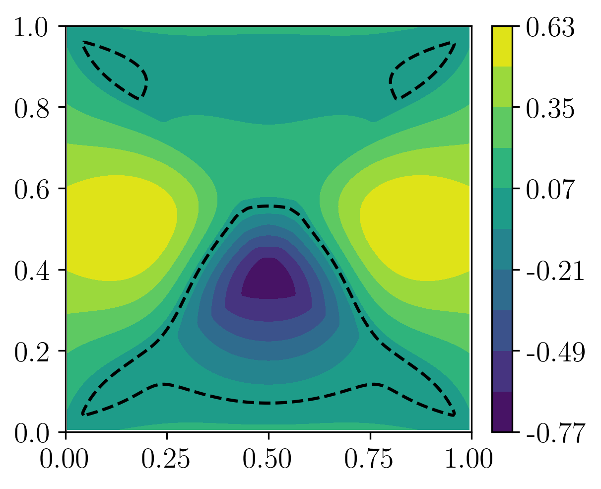
Due to the symmetry, there are actually two -maximizing locations: and Figure 4(a) shows centered at the former. The corresponding expected profit can be found in Figure 4(b), with the dashed line showing .

Subsection 6.4 Example 4: allocating surveillance resources
Given the non-unique maxima in Example 3, we now suppose that PAMs decide to build a separate drone station at each of these two locations. The next question is how to share the surveillance resources between them. Assuming that the overall number of drones is fixed and that the detection rate generated by each station is proportional to the number of drones stationed there, any allocation corresponds to choosing with and defining
with chosen to ensure . For each we compute the on a uniform rectangular grid with , , and . A grid search over 101 values of is used to find the -maximizing allocation. As in the previous example, the answer is not unique: both and are optimal.
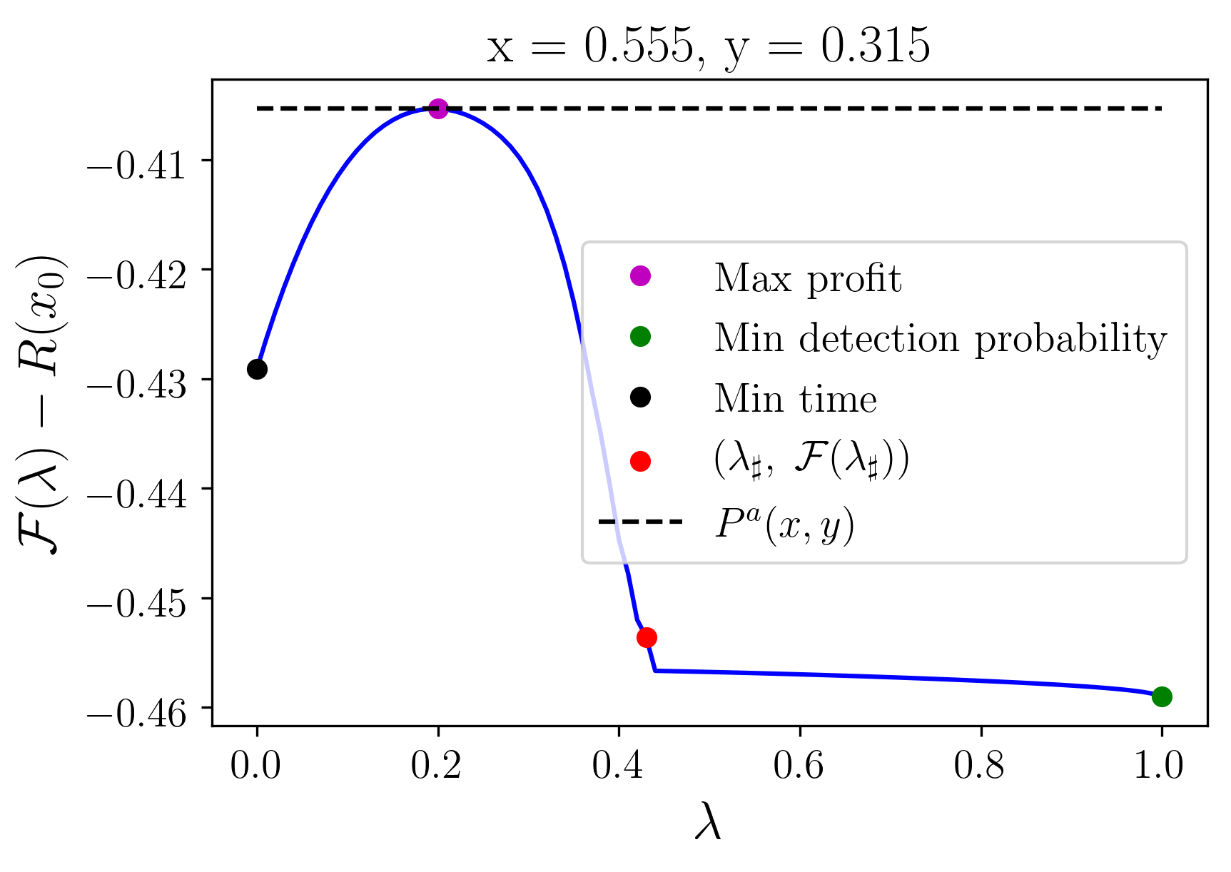
For the first of these, Figure 5(a) shows a contour plot of along with four different Pareto-optimal paths starting from an extraction point . The path maximizing the expected profit is shown in magenta, the path minimizing the probability of detection is shown in green, and the path minimizing the time of travel is shown in black. The red path corresponds to the “nearly optimal” of the linearized- problem, as discussed in Remark 4. The corresponding expected profit can be found in Figure 5(b), with the dashed line showing .


In Figure 6, we consider the -optimization problem (23) for the same extraction point in detail. Figure 6(a) shows the -optimal payoffs in blue, with the maximum profit ) as a black dashed line. The choice of path based on is clearly far from optimal, which is not surprising since is not small. The linearized- approach significantly overestimates the probability of detection along all trajectories. In fact, if we were to base the estimated “profit” on the formula (17) would yield an even more pessimistic
Figure 6(b) shows the Pareto Front for the same The color of points in in 6(a) and 6(b) matches the color of the corresponding paths in 5(a).

Subsection 6.5 Example 5: exploiting patrol gaps
The main purpose of this example is to highlight the differences in post-extraction trajectories between Models A and G. The domain is again the unit square , with a uniform speed of . The benefit function is
and can be seen in Figure 7(a). The patrol density is a sum of eight Gaussians with different means and standard deviations and can be seen in Figure 7(b).
In Figure 7(c) we see the expected profit from Model A computed on a uniform rectangular grid with , and . The optimal post-extraction trajectory corresponding to is shown in magenta, and is shown in orange.
In Figure 7(d) we see the expected profit from Model G computed on the same grid, and is shown in orange. While is only slightly larger than , a significant difference can be seen in the post-extraction trajectories. The solid magenta line represents the optimal post-extraction (pre-detection) trajectory starting from The dotted magenta lines show possible post-detection trajectories from three different positions. Since , every post-detection trajectory is just a straight line to the closest point on .


Subsection 6.6 Example 6: Yosemite National Park
Here we use the domain and terrain data from Yosemite National Park. To facilitate the comparison, we use the same and defined in [4].
The benefit function shown in Figure 8(a) is where The banded patrol density shown in Figure 8(b) is defined by
where is selected based on .
The extractors’ isotropic speed of motion is shown in Figure 8(c) and depends on the slope of the elevation map . Namely, is the grade in the direction of and
| (26) |
This example was computed on a uniform rectangular grid with , , and . The expected profit can be seen in Figure 8(d). The red dashed line corresponds to the boundary of the “high value region”
| (27) |
with This definition is chosen for the sake of direct comparison with Figure 9 in [4] since that paper does not consider the cost of pre-extraction trajectories and their definition of pristine region is also different.


Under our interpretation of the extraction criteria, the extractors will target more than of the park, and the patrol budget is clearly insufficient. We repeat this experiment with a higher see Figure 9.
This example presents a non-trivial Pareto Front since the detection rate is -banded (rather than -banded) and the time-optimal paths are generally not detection-minimizing. As a result, the predicted profit in Model A is different from Model G, but the differences are not very large here; e.g., even with the higher patrol budget used in Figure 9.
It is also worth noting that the definition (26) results in very small (and occasionally even zero up to machine precision) on all steep parts of . As a result, the cost of targeting those points becomes extremely high even if everything around them is extracted. This explains the “noisy” look of in Figure 8(d) and in Figure 9. Such un-extractable points are not identified in Figure 9b of [4] since they are masked by the -interpolation procedure used in that paper.


Subsection 6.7 Example 7: Kangaroo Island
We use the domain and terrain data corresponding to Kangaroo Island with the same and considered in [4].
The functions and are defined exactly as in Example 6; see Figures 10(a) and 10(c). The detection rate is a positive constant from to and zero elsewhere, scaled to match the budget see Figure 10(b).
This example was computed on a uniform rectangular grid with , , and . The expected profit can be seen in Figure 10(d). The red dashed line corresponds to the boundary of the “high value region” defined in (27) and can be compared with Figure 12b in [4]. Again, almost the entire is targeted by the extractors. Since the terrain is mostly flat, this remains true even with a much higher budget ; see Figure 11(a).
In Figure 11(b) we examine Model G with the same parameters. Since a detection is much less costly in Model G, the extractors are even more willing to enter the patrolled area, and the pristine area (shown in orange) is about two times smaller than in Figure 11(a).


Section 7 Conclusions
We have presented two control-theoretic models of illegal resource extraction counteracting the detection efforts of Protected Area Managers (PAMs). The perpetrators are assumed to choose potential extraction sites based on their expected profit. They take into account the distribution of resources, the geometry and terrain of the protected area , and the localized detection rate due to PAMs’ patrol activities. The cost of extracting at is based on a roundtrip The two portions of the trip usually follow different paths. The path is selected to minimize the time and hardship of travel, while on the way back () these are balanced against the expected losses resulting from a possible detection by PAMs.
A detection is always followed by confiscation of resources carried by the extractor. But the details of how and when a confiscation happens significantly influence the perpetrators’ decision making process. Our “Model G” assumes that the extractors are spotted by ground patrols with an immediate capture/confiscation after their detection. It is further assumed that after the confiscation the extractors switch to the quickest path to leave the protected area. We find their best pre-detection trajectories by recasting this as an optimal control of a suitable randomly-terminated process. Our “Model A” assumes that the extractors are spotted by aerial patrols but remain oblivious when this happens, continuing along their originally chosen trajectory until they are captured at The key challenge of this application is the impossibility of writing a single running cost to be integrated along the post-extraction path unless we resort to a linearizing approximation for the probability of detection (see Remark 2) or agree to increase the dimension of our planning space (see Remark 3). We show that the former often leads to very inaccurate predictions while the latter leads to expensive numerical methods. Instead, we opt to use the techniques of multiobjective dynamic programming on the original domain , resulting in an accurate and efficient numerical implementation. Our method is illustrated on a range of examples, with two of them based on real terrain maps from Yosemite National Park in California and Kangaroo Island in South Australia. In each case, we compute the perpetrators’ expected profit from all possible extraction sites as well as the “pristine” region not affected by extraction. We also show that Model G generally results in higher expected profits, smaller and different post-extraction trajectories.
Many of our modeling assumptions were made primarily for the simplicity of exposition and could be easily relaxed in the future. For example, it would not be hard to incorporate extractor’s preferences for starting and terminal positions on One could also easily model the time needed to extract at each site and the resulting increase in the risk of detection. It would be similarly trivial to include additional fines in case of detection/capture. Following [4], we have assumed that the extractors’ speed of motion is isotropic. I.e., if is the elevation map, the speed was based on the grade in the direction of rather than on the grade in the chosen direction of motion . In reality, a pedestrian’s speed should depend on both, particularly for moderate Any such model would replace Eikonal PDEs with anisotropic HJB equations. Efficient numerical methods for the latter have also been developed both in Fast Marching [36, 2, 27] and Fast Sweeping [37, 24] frameworks.
While our current implementation is sequential, we note that it would be easy to build a parallel algorithm with excellent scalability for computing : for each specific or , the value function could be computed by a separate CPU core. The resulting speed-up will be very useful in optimizing the choice of detection rate to maximize the area of while staying within PAMs’ enforcement/surveillance budget. In the current paper we perform some of this by straightforward grid searches, but a more general -optimization will require higher computational efficiency. The problem of optimally allocating surveillance resources across several patrol stations (e.g., Example 4) will become particularly expensive as the number of stations grows. We believe that an efficient solution will be based on generalizing our recent work on surveillance-evasion games [20, 11].
We conclude by listing two significant challenges not tackled in the current paper. Firstly, a “single period” assumption for this Stackelberg game is rather limiting. As extractors continue degrading the protected area , the distribution of resources changes and PAMs should accordingly re-allocate the surveillance resources, adjusting to increase the pristine region Secondly, in practice the detection rate is not chosen directly but results from implementing specific surveillance strategies (e.g., choices of particular patrol trajectories and patrol frequencies). It would be far more realistic and more difficult to optimize those strategies directly.
Acknowledgements. We are very grateful to all authors of [4] for answering our questions about their model and for sharing the terrain data used in their numerical experiments. The current paper was written during AV’s sabbatical visit to ORFE/Princeton, and he would like to thank ORFE for its hospitality.
References
- [1] H. J. Albers, Spatial modeling of extraction and enforcement in developing country protected areas, Resource and Energy Economics, 32 (2010), pp. 165–179.
- [2] K. Alton and I. M. Mitchell, An ordered upwind method with precomputed stencil and monotone node acceptance for solving static convex Hamilton-Jacobi equations, Journal of Scientific Computing, 51 (2012), pp. 313–348.
- [3] J. Andrews and A. Vladimirsky, Deterministic control of randomly-terminated processes, Interfaces and Free Boundaries, 16 (2014), pp. 1–40.
- [4] D. J. Arnold, D. Fernandez, R. Jia, C. Parkinson, D. Tonne, Y. Yaniv, A. L. Bertozzi, and S. J. Osher, Modeling environmental crime in protected areas using the level set method, arXiv preprint arXiv:1808.03228, (2018).
- [5] M. Bardi and I. Capuzzo-Dolcetta, Optimal control and viscosity solutions of Hamilton-Jacobi-Bellman equations, Springer Science & Business Media, 2008.
- [6] G. Barles and P. E. Souganidis, Convergence of approximation schemes for fully nonlinear second order equations, Asymptotic analysis, 4 (1991), pp. 271–283.
- [7] T. J. Barth and J. A. Sethian, Numerical schemes for the Hamilton–Jacobi and level set equations on triangulated domains, Journal of Computational Physics, 145 (1998), pp. 1–40.
- [8] M. Boué and P. Dupuis, Markov chain approximations for deterministic control problems with affine dynamics and quadratic cost in the control, SIAM J. Numer. Anal, 36 (1998), pp. 667–695.
- [9] E. K. Boukas, A. Haurie, and P. Michel, An optimal control problem with a random stopping time, Journal of Optimization Theory and Applications, 64 (1990), pp. 471–480.
- [10] A. Bressan and B. Piccoli, Introduction to the mathematical theory of control, vol. 1, American institute of mathematical sciences Springfield, 2007.
- [11] E. Cartee, L. Lai, Q. Song, and A. Vladimirsky, Time-dependent surveillance-evasion games, preprint arXiv:1903.01332, (2019).
- [12] A. Chacon and A. Vladimirsky, Fast two-scale methods for eikonal equations, SIAM Journal on Scientific Computing, 34 (2012), pp. A547–A578.
- [13] , A parallel two-scale method for eikonal equations, SIAM Journal on Scientific Computing, 37 (2015), pp. A156–A180.
- [14] Z. Clawson, X. Ding, B. Englot, T. A. Frewen, W. M. Sisson, and A. Vladimirsky, A bi-criteria path planning algorithm for robotics applications, preprint arXiv:1511.01166, (2015).
- [15] M. G. Crandall and P.-L. Lions, Viscosity solutions of Hamilton-Jacobi equations, Transactions of the American mathematical society, 277 (1983), pp. 1–42.
- [16] I. Das and J. E. Dennis, A closer look at drawbacks of minimizing weighted sums of objectives for Pareto set generation in multicriteria optimization problems, Structural optimization, 14 (1997), pp. 63–69.
- [17] A. Desilles and H. Zidani, Pareto front characterization for multi-objective optimal control problems using Hamilton-Jacobi approach, preprint, (2018).
- [18] E. W. Dijkstra, A note on two problems in connexion with graphs, Numerische mathematik, 1 (1959), pp. 269–271.
- [19] F. Fang, T. H. Nguyen, R. Pickles, W. Y. Lam, G. R. Clements, B. An, A. Singh, B. C. Schwedock, M. Tambe, and A. Lemieux, PAWS - a deployed game-theoretic application to combat poaching., AI Magazine, 38 (2017), pp. 23–36.
- [20] M. Gilles and A. Vladimirsky, Surveillance-evasion games under uncertainty, preprint arXiv:1812.10620, (2018).
- [21] A. Haurie, A multigenerational game model to analyze sustainable development, Annals of Operations Research, 137 (2005), pp. 369–386.
- [22] A. Haurie and F. Moresino, A stochastic control model of economic growth with environmental disaster prevention, Automatica, 42 (2006), pp. 1417–1428.
- [23] M. P. Johnson, F. Fang, and M. Tambe, Patrol strategies to maximize pristine forest area, in Twenty-Sixth AAAI Conference on Artificial Intelligence, 2012.
- [24] C. Kao, S. Osher, and Y. Tsai, Fast sweeping methods for static hamilton–jacobi equations, SIAM Journal on Numerical Analysis, 42 (2005), pp. 2612–2632.
- [25] D. Kar, B. Ford, S. Gholami, F. Fang, A. Plumptre, M. Tambe, M. Driciru, F. Wanyama, A. Rwetsiba, M. Nsubaga, et al., Cloudy with a chance of poaching: Adversary behavior modeling and forecasting with real-world poaching data, in Proceedings of the 16th Conference on Autonomous Agents and MultiAgent Systems, International Foundation for Autonomous Agents and Multiagent Systems, 2017, pp. 159–167.
- [26] A. Kumar and A. Vladimirsky, An efficient method for multiobjective optimal control and optimal control subject to integral constraints, Journal of Computational Mathematics, (2010), pp. 517–551.
- [27] J.-M. Mirebeau, Efficient fast marching with Finsler metrics, Numerische mathematik, 126 (2014), pp. 515–557.
- [28] I. M. Mitchell and S. Sastry, Continuous path planning with multiple constraints, in 42nd IEEE International Conference on Decision and Control (IEEE Cat. No. 03CH37475), vol. 5, IEEE, 2003, pp. 5502–5507.
- [29] S. Osher and J. A. Sethian, Fronts propagating with curvature-dependent speed: Algorithms based on Hamilton-Jacobi formulations, Journal of Computational Physics, 79 (1988), pp. 12 – 49.
- [30] J. Qian, Y.-T. Zhang, and H.-K. Zhao, Fast sweeping methods for eikonal equations on triangular meshes, SIAM Journal on Numerical Analysis, 45 (2007), pp. 83–107.
- [31] E. J. Robinson, H. J. Albers, and J. C. Williams, Spatial and temporal modeling of community non-timber forest extraction, Journal of Environmental Economics and Management, 56 (2008), pp. 234 – 245.
- [32] E. J. Z. Robinson, India’s disappearing common lands: Fuzzy boundaries, encroachment, and evolving property rights, Land Economics, 84 (2008), pp. 409–422.
- [33] J. A. Sethian, A fast marching level set method for monotonically advancing fronts, Proceedings of the National Academy of Sciences, 93 (1996), pp. 1591–1595.
- [34] , Fast marching methods, SIAM review, 41 (1999), pp. 199–235.
- [35] J. A. Sethian and A. Vladimirsky, Fast methods for the Eikonal and related Hamilton–Jacobi equations on unstructured meshes, Proceedings of the National Academy of Sciences, 97 (2000), pp. 5699–5703.
- [36] , Ordered upwind methods for static Hamilton–Jacobi equations: Theory and algorithms, SIAM Journal on Numerical Analysis, 41 (2003), pp. 325–363.
- [37] Y.-H. R. Tsai, L.-T. Cheng, S. Osher, and H.-K. Zhao, Fast sweeping algorithms for a class of Hamilton–Jacobi equations, SIAM Journal on Numerical Analysis, 41 (2003), pp. 673–694.
- [38] J. N. Tsitsiklis, Efficient algorithms for globally optimal trajectories, IEEE Transactions on Automatic Control, 40 (1995), pp. 1528–1538.
- [39] H. Zhao, A fast sweeping method for eikonal equations, Mathematics of computation, 74 (2005), pp. 603–627.