Pentaquarks

The excitation spectrum of a charm-anticharm state is well described by a semi-relativistic phenomenological potential (Cornell potential) cornell, developed in the 70’s after the discovery of the $J/\psi$ and other charmonia states. It comprises a sum of three terms:

$$V(r)=-\frac{4}{3}\frac{\alpha_{s}(r)}{r}+\sigma r+\delta(1/r^{2}),$$

(1)

where the first is a short-distance colour potential, the second is a long-distance confinement term and the third includes spin-spin and spin-orbit corrections. This potential is found to be particularly accurate to describe the spectrum of excited $c\bar{c}$ and $b\bar{b}$ states, as well as predict new states before their observation. However, in the last two decades a large number of states has been discovered, which are compatible with being composed by - at least- a $c\bar{c}$ pair as constituent quarks as they all decay into a final state with a charmonium; however, they do not fit in the expected spectrum given their mass and other properties, such as decay and production rates or quantum numbers, which would be expected from a pure $c\bar{c}$ state. All these states are labelled as exotic states. Fig. 1 shows the charmonium spectrum, including all exotic states, as it was in 2017.

The first exotic state ever observed is the $X(3872)$ (recently renamed $\chi_{c1}(3872)$), from data analysed by the Belle experiment, in 2003 belleX. Its mass, $3871.69$ MeV/$c^{2}$, is not close to any predicted $c\bar{c}$ state. Its width is extremely narrow, and indeed it is limited by experimental resolution to be less than 1.2 MeV/$c^{2}$; this is unexpected for a $c\bar{c}$ state above the open charm mass threshold. Moreover, the measured radiative decay rates seem not match predictions Xrad, and it has been observed to decay into two final states with different isospin ($J/\psi\rho^{0}$ and $J/\psi\omega$) with similar rates. Given its proximity to the $D^{0}\bar{D}^{*0}$ mass threshold, it is believed that the $X(3872)$ is a good candidate for a bound state of four quarks (tetraquark), although the binding mechanism is still unknown (see next section). Many of the observed exotic states are tetraquark candidates, and in particular the $Z_{c}$ states (for instance, $Z_{c}(4430)$) which are charged and must have a minimal constituent quarks content of $c\bar{c}d\bar{u}$. Similarly, the charged states discovered by the LHCb experiment in the $J/\psi p$ final state must have a minimal quark content of $uudc\bar{c}$; therefore, they are pentaquark candidates.

More information on exotic states, along with details about the models described in the next section, can be found in Ref. XYZ.

Several models have been proposed to describe the multiquark candidates. The two main interpretations are described in this section as an example.

In the compact multiquark picture, the quarks are tightly bound into a colour-neutral state. Large widths are expected, as well as many isomultiplet states with similar mass. While this model can explain the large prompt production of some candidates, it fails to describe the narrow width observed in many exotic states; furthermore, no isospin partner has ever been found.

In the molecular picture, the exotic state is described by a mesonic - or baryonic - molecule. The bound state is expected to have mass a little below the mass threshold necessary to decay strongly into its components; therefore, at least one couple of quarks must change their confining partners before the molecule can decay, and this leads to long-lived states (i.e. narrow widths). Few states are predicted, due to the low binding energy required to form them, which allows the existence of only low orbital momentum states, perhaps only S-wave. It is believed that the binding energy is too small to account for the large prompt production in colliders. Other models are in principle allowed, as well as mixture of different models.

The LHCb experiment has analysed $\Lambda_{b}^{0}\to J/\psi K^{-}p$ decays from $pp$ collisions using the full Run 1 dataset, which comprises 3 fb^-1 of data collected at 7 and 8 TeV during 2011 and 2012 penta1. This channel is expected to be dominated by resonant $\Lambda^{*}\to K^{-}p$ decays; however, a large structure is visible also in the $m_{J/\psi p}$ spectrum. In order to investigate the nature of said structure, it is necessary to chech whether this can be a result of reflections in the Dalitz plot caused by the expected $\Lambda^{*}$ activity. In order to do so, 14 well established $\Lambda^{*}$ are taken into account in building a six-dimensional amplitude model, which includes 5 decays angles in the helicity formalism helicity and $m_{Kp}$. The amplitude fit is performed following two strategies: first, a sum of a double-sided Hypatia function hypatia and a background component, modeled on sidebands, is fit to the $\Lambda_{b}^{0}$ peak. From this fit, signal weights are extracted with the $sPlot$ method splot. The full amplitude model is then fit to background-subtracted data, obtained by applying the aforementioned weights. The fit to the $\Lambda_{b}^{0}$ peak is shown in Fig. 2. For the second strategy, the amplitude model is fit to unweighted data, with an additional background component, within $\pm 2\sigma$ of the $\Lambda_{b}^{0}$ mass peak. The two strategies give compatible results.

By studying the $m_{J/\psi p}$ projection of the six-dimensional fit, shown in Fig. 3, it is observed that the fit does not describe the data well unless two more contributions are added: a broad state, $\Gamma=205\pm 18$ MeV, with mass 4380 MeV/$c^{2}$, and a narrow state, $\Gamma=39\pm 5$ MeV, with mass 4450 MeV/$c^{2}$. These two states are labelled, respectively, $P_{c}(4380)^{+}$ and $P_{c}(4450)^{+}$. Their favourite $J^{PC}$ assignment is $3/2^{-}$ and $5/2^{+}$, though combinations ($3/2^{+}$, $5/2^{-}$) and ($5/2^{+}$, $3/2^{-}$) are also possible. The singificance of each contribution is, respectively, 9$\sigma$ and 12$\sigma$.

The analysis described in Section II.1 is repeated using a different, model-independent approach independent. This consists in describing the bidimensional plane ($m_{Kp}$,$\cos\theta_{\Lambda^{*}}$) by expanding the helicity angle $\theta_{\Lambda^{*}}$ in Legendre polynomials,

$$\frac{dN}{d(\cos\theta_{\Lambda^{*}})}=\sum_{l=0}^{l_{max}}a_{l}P_{l}(\cos\theta_{\Lambda^{*}}),$$

(2)

where $P_{l}$ is the Legendre polynomial of order $l$ and the coefficients of the expansion (Legendre moments) are defined as

$$a_{l}=\frac{2l+1}{2}\int_{-1}^{+1}\frac{dN}{d(\cos\theta_{\Lambda^{*}})}P_{l}(\cos\theta_{\Lambda^{*}})\text{ }d\cos\theta_{\Lambda^{*}}.$$

(3)

The moments $a_{l}$ are extracted from efficiency-corrected, background-subtracted data by quadratically interpolate the $m_{Kp}$ histogram. Under the hypothesis that all $\Lambda_{b}\to J/\psi pK^{-}$ decays proceeds via intermediate $\Lambda^{+}$, $\Sigma^{*}$ or non resonant $K^{-}p$, each component cannot contribute to moments of rank higher than $2J_{max}$, where $J_{max}$ is the highest spin of any $K^{-}p$ contribution at a given $m_{Kp}$ value; therefore, $l_{max}$ in Eq. 2 depends on the spin of the intermediate resonances that might be available at a certain value of the $K^{-}p$ mass. This is summarised in Fig. 4.

If exotic contributions are present, then the hypothesis under which the calculation of the Legendre moments has been performed will not be valid; therefore, the $m_{J/\psi p}$ distribution will not be well described by the expansion. This is indeed what is observed, as can be seen in Fig. 5: the discrepance is calculated using a second Legendre expansion with an unphysically large $l_{max}=31$ which describes the statistical significant features of data; its significance is calculated to be $9\sigma$, thus confirming the presence of contributions to $\Lambda_{b}\to J/\psi pK^{-}$ decays, either due to exotic resonances or rescattering effects. The latter are investigated and excluded in separate results, described in the next Section.

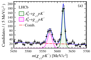
If $P_{c}^{+}(4450)$ is a real resonance, then it could in principle decay to $\chi_{c1}p$, thus neglecting final-state interactions between $\chi_{c1}$ and $p$. The LHCb Collaboration has analysed the full Run 1 dataset searching for resonant structures in $\Lambda_{b}^{0}\to\chi_{c1}pK^{-}$ decays chic. The number of observed signal decays, N$(\Lambda_{b}^{0}\to\chi_{c1}pK^{-})=453\pm 25$, is not large enough to allow an analysis of the $m_{\chi_{c1}p}$ spectrum; this will be updated with the addition of Run 2 data. The fit used to extract the signal yield is shown in Fig 6. Nonetheless, this first investigation on this channel lead to the first observation of the decays $\Lambda_{b}^{0}\to\chi_{c1,2}pK^{-}$ and first measurement of their relative branching fraction:

	$\displaystyle\frac{\mathcal{B}(\Lambda_{b}^{0}\to\chi_{c1}pK^{-})}{\mathcal{B}(\Lambda_{b}^{0}\to J/\psi pK^{-})}=0.242\pm 0.014\pm 0.013\pm 0.009,$
	$\displaystyle\frac{\mathcal{B}(\Lambda_{b}^{0}\to\chi_{c2}pK^{-})}{\mathcal{B}(\Lambda_{b}^{0}\to J/\psi pK^{-})}=0.248\pm 0.020\pm 0.014\pm 0.009.$

An observation of the $P_{c}(4450)^{+}\to J/\psi p$ decay from $\Lambda_{b}^{0}\to J/\psi p\pi^{-}$ decays would not only confirm the existence of an unexpected contribution, but also its exotic nature. In fact, while the Cabibbo-favoured channel is dominated by $\Lambda^{*}\to pK^{-}$ decays, the Cabibbo-suppressed channel is dominated by intermediate excited nucleons decays, $N^{*}\to p\pi^{-}$. The masses of the known excited nucleons all lie outside the range that would allow a kinematic enhancement due to rescattering; therefore, this mechanism would be much harder to accommodate in this picture.

The analysis is performedy with the full LHCb Run 1 dataset cabibbo. The analysis strategy is similar to the one described in Section II.1: 14 well established $N^{*}$ resonances are used to build a six-dimensional amplitude model, using five decay angles in the helicity formalism and the $\pi^{-}p$ invariant mass; thanks to the $\Delta I=1/2$ rule deltaI, the $\Lambda^{*}\to p\pi^{-}$ contributions are suppressed. This model is then fit to background-subtracted data, obtained by extracting signal weights with the $sPlot$ technique via a fit to the $\Lambda_{b}^{0}$ peak. Analogously to the Cabibbo-favoured case, the amplitude fit is found to be significantly improved when the two previously observer pentaquark candidates, $P_{c}(4380)^{+}$ and $P_{c}(4450)^{+}$, along with a $Z_{c}(4200)^{-}\to J/\psi\pi^{-}$ contribution, are added to the fits. The fit is shown in Fig. 7, including the cut $m_{p\pi^{-}}>1.8$ GeV/$c^{2}$ in order to enhance the exotic components. The combined significance obtained by adding the three exotic contributions is calculated to be 3.1$\sigma$. The production rates are found to be compatible with expectations based on the analysis of the Cabibbo-favoured channel.

The Belle Collaboration has analysed 915 fb^-1 of data collected at the $\Upsilon(4S)$ and $\Upsilon(5S)$ peaks to search for strange-flavoured pentaquarks in the strange-flavour analogue channel of the $P_{c}^{+}$ discovery, i.e. $\Lambda_{c}^{+}\to\phi p\pi^{0}$ belle. The hypothetic $P_{s}^{+}$ could be observed as a peak in the $m_{\phi p}$ spectrum, provided that the same production mechanism as the charm pentaquarks holds and if its mass is $m_{P_{s}^{+}}<m_{\Lambda_{c}^{+}}-m_{\pi^{0}}$. To extract the signal yield, a bidimensional fit to the variables $m_{K^{+}K^{-}p\pi^{0}}$ and $m_{K^{+}K^{-}}$ is performed. The number of signal events is found to be $148.4\pm 61.8$. A sum of a relativistic Breit-Wigner and a phase space distribution determined from simulation is then fitted to the background-subtracted $m_{\phi p}$ spectrum, in a 20 MeV/$c^{2}$ mass window around the $\phi$ peak, in order to search for a putative $P_{s}^{+}$ peak. No clear evidence is found, and an upper limit at 90% CL is set on the product of the branching fractions, normalised using $\Lambda_{c}^{+}\to pK^{-}\pi^{+}$ decays,

$$\mathcal{B}(\Lambda_{c}^{+}\to P_{s}^{+}\pi^{0})\times\mathcal{B}(P_{s}^{+}\to\phi p)<8.3\times 10^{-5}.$$

The fit to the $m_{\phi p}$ spectrum is shown in Fig. 8. As a reference, for the $P_{c}(4450)^{+}$ discovery the analogous quantity reads:

$$\mathcal{B}(\Lambda_{b}^{0}\to P_{c}^{+}K^{-})\times\mathcal{B}(P_{c}^{+}\to J/\psi p)=(1.3\pm 0.4)\times 10^{-5}.$$

According to the Skyrme model skyrme, the heavier the consituent quarks are, the more tightly bound the pentaquark state is; furthermore, no search for $b$-flavoured pentaquark exists in literature. The LHCb Collaboration has analysed the full Run 1 dataset to search for four possible, weakly-decaying $b$-flavoured pentaquarks bpenta. The weak decay channels, quark contents and mass search windows are summarised in Tab. 1. The mass windows are chosen to be below the strong decays thresholds, and the subscript on each state indicates the final state the pentaquark would predominantly decay into if it had sufficient mass to decay strongly in those states.

While there are many possible decay modes of these states, the analysis is focussed only on $b\to c\bar{c}s$ processes in order to have a $J/\psi$ in the final state, for which the LHCb experiment has large reconstruction efficiencies and reduced backgrounds.

No signal is observed for any of the final states considered, and upper limits at 90% CL are set on the products of the production cross sections and the branching ratios, normalised using $\Lambda_{b}^{0}\to J/\psi pK^{-}$ decays. The upper limits as a function of the invariant masses in the search windows are shown in Fig. 9.

References

- (1) E. Eichten et al., Phys. Rev. D21, 203 (1980).
- (2) S. Choi et al. (Belle Collaboration), Phys. Rev. Lett. 91, 262001 (2003).
- (3) Y. Dong et al., J. Phys. G: Nucl. Part. Phys. 38 015001 (2011).
- (4) S. L. Olsen et al., Rev. Mod. Phys. 90, 015003 (2018).
- (5) H. Chen et al., Physics Reports 639, 1-121 (2016).
- (6) R. Aaij et al. (LHCb Collaboration), Phys. Rev. Lett. 115, 072001 (2015).
- (7) S. U. Chung, Report No. CERN-71-08; J. D. Richman, Report No. CALT-68-1148; M. Jacob and G. C. Wick, Ann. Phys. (N.Y.) 7, 404 (1959).
- (8) D. Martinez Santos and F. Dupertuis, Nucl. Instrum. Methods Phys. Res., Sect. A764, 150 (2014).
- (9) M. Pivk and F. R. Le Diberder, Nucl. Instrum. Meth. A555 356-369 (2005).
- (10) R. Aaij et al. (LHCb Collaboration), Phys. Rev. Lett. 117, 082002 (2016).
- (11) F. Guo et al., Phys. Rev. D92, 071502 (2015).
- (12) E. Wang et al., Phys. Rev. D93, 094001 (2016).
- (13) R. Aaij et al. (LHCb Collaboration), Phys. Rev. Lett. 119, 062001 (2017).
- (14) R. Aaij et al. (LHCb Collaboration), Phys. Rev. Lett. 117, 082003 (2016).
- (15) J.F. Donoghue et al., Phys. Rev. D21, 186 (1980).
- (16) B. Pal et al. (Belle Collaboration), Phys. Rev. D96, 051102 (2017).
- (17) T. H. R. Skyrme, 260 Proc. R. Soc. Lond. A (1961).
- (18) R. Aaij et al. (LHCb Collaboration), Phys. Rev. D97, 032010 (2018).
- (19) R. Aaij et al. (LHCb Collaboration), Phys. Rev. Lett. 122, 222001 (2019).