跳到论文正文
W Papers独立论文阅读器 arXiv:1906.09070 论文正文 计算阅读时间 · 0%
引用这篇论文根据当前论文元数据生成,正式投稿前建议核对。


License: arXiv.org perpetual non-exclusive license
arXiv:1906.09070v2 [math.DS] 10 Jun 2021

Building oscillatory chemical reaction networks by adding reversible reactions

Murad Banaji11 1 Middlesex University, London, Department of Design Engineering and Mathematics. m.banaji@mdx.ac.uk.
Abstract

We show that if a chemical reaction network (CRN) admits nondegenerate (resp., linearly stable) oscillation, and we add new reversible reactions involving new species to this CRN, then the new CRN so created also admits nondegenerate (resp., linearly stable) oscillation provided certain mild and easily checked conditions are met. This claim that the larger CRN “inherits” oscillation from the smaller one, provided it is built from the smaller CRN in an appropriate way, follows an analogous result involving multistationarity. It also adds to a number of prior results on the inheritance of oscillation; these collectively often allow us to determine the capacity of a given network for oscillation based on an analysis of its subnetworks.

keywords
Oscillation; chemical reaction networks MSC. 80A30; 37C20; 37C27; 34D15

1 Introduction and statement of the main result

A mathematically interesting and practically important question is when we can infer some dynamical behaviour in a network model based on knowledge that this behaviour occurs in some model of a subnetwork. Results in this area focussed on chemical reaction networks (CRNs), for example in [1, 2, 3, 4, 5, 6], have illustrated that this is a rather subtle question. Some intuitively plausible claims turn out to be hard to prove, or to be false. This paper contributes to this literature. The dynamical behaviour of interest here is oscillation, and the main result to be proved (Theorem 1 below) was conjectured to hold in the concluding sections of [6]; however the proof turned out to be somewhat harder than expected.

The work here can be motivated by the following natural questions about sequestration or inhibition. To make the arguments concrete, consider any standard biochemical model exhibiting stable oscillations, such as the classical two-pool calcium model of Goldbeter et al [7] or models of glycolytic oscillations [8]. Now suppose we introduce a reversible “sequestration” process where one of the existing chemical species can bind reversibly to some species, either already in the model or new, to create a new inactive complex. Equivalently (from a mathematical point of view), we introduce an allosteric inhibitor which binds reversibly to some existing species converting it to an inactive form. Could such a process, with certainty, destroy stable oscillation? The answer is no – maintaining the kinetics of the original reactions, the model will still stably oscillate if we choose mass action kinetics and appropriate rate constants for the inhibition/sequestration process. This claim is intuitively plausible. The idea is that provided (i) the binding and unbinding rates are fast so the new reaction is trying hard to equilibriate, and (ii) the ratio of rates is chosen so the bound, inactive, form has low equilibrium concentration, then the dynamics of the enlarged model projected onto the original species space is “close” to that of the original model, and stable oscillation should survive by perturbation arguments.

Theorem 1 of this paper is much more general than this motivating discussion suggests, but is guided by the desire to find under what circumstances similar arguments work. The Theorem states that we can build a new oscillatory netork by adding into an existing oscillatory network new reversible reactions, but with a caveat: some new species must figure nondegenerately in the new reactions. This condition is made precise later, but can easily be illustrated in the special case of a single added reaction, when it becomes: “there must be a net change in at least one new species in the added reaction”. Example 1.1 provides a simple illustration of the result in this special case. Meanings of the terms, and assumptions about reaction kinetics, will follow later.

Example 1.1.

Suppose that we have a CRN ℛ\mathcal{R} on chemical species X1,…,XnX_{1},\ldots,X_{n} admitting linearly stable oscillation. We now build a larger CRN ℛ′\mathcal{R}^{\prime} by adding to ℛ\mathcal{R} a reaction ℛ0\mathcal{R}_{0} involving some new species. Then, for example:

  • (i)

    If ℛ0\mathcal{R}_{0} is X1+Xn+1⇌2​Xn+1X_{1}+X_{n+1}\rightleftharpoons 2X_{n+1} then ℛ′\mathcal{R}^{\prime} also admits linearly stable oscillation: there is a net change in the new species Xn+1X_{n+1} in the added reaction.

  • (ii)

    If ℛ0\mathcal{R}_{0} is X1+Xn+1⇌Xn+1+Xn+2X_{1}+X_{n+1}\rightleftharpoons X_{n+1}+X_{n+2} then ℛ′\mathcal{R}^{\prime} admits linearly stable oscillation: there is a net change in the new species Xn+2X_{n+2} in the added reaction.

  • (iii)

    If ℛ0\mathcal{R}_{0} is X1+Xn+1⇌Xn+1X_{1}+X_{n+1}\rightleftharpoons X_{n+1} then we cannot conclude from Theorem 1 that ℛ′\mathcal{R}^{\prime} admits oscillation: there is a new species involved, but the added reaction does not cause any net change in this new species.

It is little surprise that perturbation theory (both regular and singular) forms the backbone of the proof of Theorem 1. The challenge which takes up the majority of our effort here is to recast the basic problem in a form amenable to geometric singular perturbation theory approaches. This requires effort since, firstly, adding reactions into a system alters the dynamics of both the new and the original model species and, secondly, various mathematical necessary conditions for the application of geometric singular perturbation theory are easily violated.

Returning to the broader context of the work, this paper contributes to the literature on oscillation in CRNs. This literature has a considerable history and includes theoretical, numerical, and algorithmic work, focussed on both ruling out oscillation, and finding oscillation or bifurcations which give rise to oscillation. It would be hard to compile a complete list of papers about, or with important implications for, oscillations in CRNs. Instead, the following is a small sample, illustrating both numerical and applied work, and some key strands of classical and modern theory: [9, 10, 11, 12, 13, 14, 15, 16, 17, 18, 19, 20, 21, 22, 23, 24]. Inheritance results of the kind here provide an important theoretical tool for guaranteeing the occurrence of oscillation in CRNs without resorting to numerical investigation.

Presenting a detailed introduction to the mathematical theory of CRNs can often take up a considerable chunk of a paper, and a minimal approach is adopted here: we intersperse key definitions into the text without much discussion. The reader is referred to some of the papers referenced above and to [25] for a more thorough background using notation and conventions close to those adopted here.

We now turn to statement of the main result. Consider a chemical reaction network ℛ\mathcal{R} involving nn species X1,…,XnX_{1},\ldots,X_{n} collectively termed XX. Let species XiX_{i} have concentration xix_{i} (i=1,…,ni=1,\ldots,n). We are interested in positive concentrations, namely x:=(x1,…,xn)t∈ℝ≫0n:={x∈ℝn:xi>0​for all​i}x:=(x_{1},\ldots,x_{n})^{\mathrm{t}}\in\mathbb{R}^{n}_{\gg 0}:=\{x\in\mathbb{R}^{n}\colon x_{i}>0\,\,\mbox{for all}\,\,i\}. Suppose that we have r0r_{0} chemical reactions involving XX, and that the iith reaction has reaction vector Γi\Gamma_{i} and reaction rate vi​(x)v_{i}(x). We assume only that vi:ℝ≫0n→ℝv_{i}\colon\mathbb{R}^{n}_{\gg 0}\to\mathbb{R} is C2C^{2}; other than this condition, the kinetics of the reactions is arbitrary. v⁡(x):=(v1​(x),…,vr0​(x))tv(x):=(v_{1}(x),\ldots,v_{r_{0}}(x))^{\mathrm{t}} is termed the reaction rate vector for the system, and Γ:=[Γ1​|⋯|​Γr0]\Gamma:=[\Gamma_{1}|\cdots|\Gamma_{r_{0}}] is termed the stoichiometric matrix of the system. Then the following system of ODEs on ℝ≫0n\mathbb{R}^{n}_{\gg 0} describes the evolution of the concentration vector xx.

x˙=Γ​v​(x),\dot{x}=\Gamma v(x)\,, (1)

Note that the RHS of (1) belongs to im​Γ\mathrm{im}\,\Gamma, a linear subspace of ℝn\mathbb{R}^{n} termed the stoichiometric subspace of the system, and consequently cosets of im​Γ\mathrm{im}\,\Gamma are invariant under the local flow defined by (1) on ℝ≫0n\mathbb{R}^{n}_{\gg 0}. The intersection of these cosets of im​Γ\mathrm{im}\,\Gamma with ℝ≫0n\mathbb{R}^{n}_{\gg 0} are termed the positive stoichiometry classes of the system.

Now let m≥1m\geq 1 and k≥0k\geq 0 be integers and suppose that we add to the system mm new reversible reactions involving m+km+k new species Y1,…,Ym+kY_{1},\ldots,Y_{m+k}, collectively termed YY. The new CRN obtained from ℛ\mathcal{R} by adding in the new reversible reactions will be termed ℛ′\mathcal{R}^{\prime}. In order to state a nondegeneracy condition on the added reactions we need to describe these reactions, and for this we introduce some notation.

Given a list of species, say X1,…,XnX_{1},\ldots,X_{n}, and a nonnegative integer vector of the same length, say c=(c1,…,cn)tc=(c_{1},\ldots,c_{n})^{\mathrm{t}}, we write c⋅Xc\cdot X for the formal sum (i.e., complex in CRN terminology) c1​X1+c2​X2+⋯+cn​Xnc_{1}X_{1}+c_{2}X_{2}+\cdots+c_{n}X_{n}. We simply write “00” for the zero complex 0​X1+⋯+0​Xn0X_{1}+\cdots+0X_{n}. Using this notation, let the new reactions be:

ai⋅X+bi⋅Y⇌ai′⋅X+bi′⋅Y,(i=1,…,m).a_{i}\cdot X+b_{i}\cdot Y\rightleftharpoons a_{i}^{\prime}\cdot X+b_{i}^{\prime}\cdot Y,\quad(i=1,\ldots,m)\,. (2)

Here ai,ai′,bia_{i},a_{i}^{\prime},b_{i} and bi′b_{i}^{\prime} are nonnegative integer vectors of length nn, nn, m+km+k and m+km+k respectively. Define a=(a1|a2​|⋯|​am)∈ℝn×ma=(a_{1}|a_{2}|\cdots|a_{m})\in\mathbb{R}^{n\times m}, with a′∈ℝn×ma^{\prime}\in\mathbb{R}^{n\times m}, b∈ℝ(m+k)×mb\in\mathbb{R}^{(m+k)\times m} and b′∈ℝ(m+k)×mb^{\prime}\in\mathbb{R}^{(m+k)\times m} defined similarly. Define α=a′−a∈ℝn×m\alpha=a^{\prime}-a\in\mathbb{R}^{n\times m} and β=b′−b∈ℝ(m+k)×m\beta=b^{\prime}-b\in\mathbb{R}^{(m+k)\times m}. α\alpha records the net stoichiometric changes of the old species XX in the added reactions. β\beta records the net stoichiometric changes of the new species YY in the added reactions and occurs in a nondegeneracy condition in Theorem 1 below. Let yiy_{i} denote the concentration of YiY_{i} (i=1,…,m+ki=1,\ldots,m+k), and define y:=(y1,…,ym+k)ty:=(y_{1},\ldots,y_{m+k})^{\mathrm{t}}. If the new reactions have reaction rate vector q:ℝ≫0n×ℝ≫0m+k→ℝmq\colon\mathbb{R}^{n}_{\gg 0}\times\mathbb{R}^{m+k}_{\gg 0}\to\mathbb{R}^{m}, then ℛ′\mathcal{R}^{\prime} evolves according to:

(x˙y˙)=(Γα0β)​(v⁡(x)q⁡(x,y))\left(\begin{array}[]{c}\dot{x}\\ \dot{y}\end{array}\right)=\left(\begin{array}[]{cc}\Gamma&\alpha\\ 0&\beta\end{array}\right)\left(\begin{array}[]{c}v(x)\\ q(x,y)\end{array}\right)\, (3)

on ℝ≫0n×ℝ≫0m+k\mathbb{R}^{n}_{\gg 0}\times\mathbb{R}^{m+k}_{\gg 0}. We are now ready to state our main result, although some of the definitions to make it precise will follow.

Theorem 1.

Suppose the CRN ℛ\mathcal{R} with evolution described by (1) has a nondegenerate (resp., linearly stable) positive periodic orbit. Let ℛ′\mathcal{R}^{\prime} be the CRN with evolution described by (3), obtained by adding in the reactions of (2) to ℛ\mathcal{R}. Suppose (i) β\beta has rank equal to mm, its number of columns, and (ii) the added reactions are given mass action kinetics. Then rate constants can be chosen for the added reactions in such a way that ℛ′\mathcal{R}^{\prime} has a nondegenerate (resp., linearly stable) positive periodic orbit.

By a positive periodic orbit, we mean a periodic orbit that lies in the (strictly) positive orthant. By a nondegenerate periodic orbit, we mean one that is hyperbolic relative to its stoichiometry class. Linearly stable is also taken to mean linearly stable relative to its stoichiometry class. Precise statement of these latter conditions is deferred to Section 3.

Theorem 1 is exactly analogous (including the condition that β\beta has rank mm) to Theorem 5 in [5], replacing “multiple positive nondegenerate (resp., linearly stable) equilibria” with “a nondegenerate (resp., linearly stable) positive periodic orbit”. The proof draws heavily both on techniques developed in [5], and on singular perturbation theory approaches which formed the basis for the proof of Theorem 4 in [6]. It is hoped that the proof of Theorem 1 provides a template for, or at least insight towards, the proof of further inheritance results on CRNs.

2 An example

The proof of Theorem 1 is constructive: it not only tells us about inheritance of oscillation, but also gives information about parameter regions at which oscillation occurs. Before the proof, we present an example illustrating the result, including how to choose parameter values at which we can observe inherited oscillation. We will re-examine in detail this example in Section 5 after presenting the proof of Theorem 1 and use it to help elucidate various ideas and quantities in the proof. Here we use it only to outline the conclusions.

In [6], the following was presented as an example of a CRN which admits stable oscillation with mass action kinetics:

X+Z​⟶k1​2​Y​⟶k2​X+Y,0​⇌k4k3​X,0​⇌k6k5​Y,0​⇌k8k7​Z.X+Z\overset{\scriptstyle{k_{1}}}{\longrightarrow}2Y\overset{\scriptstyle{k_{2}}}{\longrightarrow}X+Y,\quad 0\overset{\scriptstyle{k_{3}}}{\underset{\scriptstyle{k_{4}}}{\rightleftharpoons}}X,\quad 0\overset{\scriptstyle{k_{5}}}{\underset{\scriptstyle{k_{6}}}{\rightleftharpoons}}Y,\quad 0\overset{\scriptstyle{k_{7}}}{\underset{\scriptstyle{k_{8}}}{\rightleftharpoons}}Z\,. (ℛ1\mathcal{R}_{1})

This is an example of a so-called fully open CRN on three species X,YX,Y and ZZ, as it includes the inflow-outflow reactions 0⇌X0\rightleftharpoons X, 0⇌Y0\rightleftharpoons Y and 0⇌Z0\rightleftharpoons Z. The reactions are labelled with their rate constants. In numerical simulations we easily find parameter regions where the CRN admits a stable periodic orbit. For example, setting k1=4,k2=3,k3=0.2,k4=2,k5=0.3,k6=2.5,k7=2.5k_{1}=4,\,k_{2}=3,\,k_{3}=0.2,\,k_{4}=2,\,k_{5}=0.3,\,k_{6}=2.5,\,k_{7}=2.5 and k8=0.2k_{8}=0.2, and choosing initial conditions X0=Y0=Z0=1X_{0}=Y_{0}=Z_{0}=1 we find the system settles, after initial transients, onto the periodic orbit shown in Figure 1. We assume that the system does indeed have a positive, linearly stable periodic orbit at these parameter values.

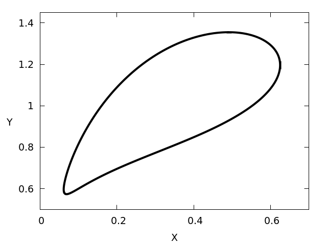
Refer to caption
Refer to caption
Figure 1: Simulation of the CRN ℛ1\mathcal{R}_{1} with mass action kinetics and rate constants as given in the text. Left. Evolution of the concentrations of XX, YY and ZZ. Right. The projection of the periodic orbit onto X−YX\mathchar 45\relax Y coordinates.

Now suppose that we add in two further reversible reactions Y⇌U+VY\rightleftharpoons U+V and U+X⇌2​V+WU+X\rightleftharpoons 2V+W involving three new species U,VU,V and WW to obtain the system

X+Z​⟶k1​2​Y​⟶k2​X+Y,   0​⇌k4k3​X,   0​⇌k6k5​Y,   0​⇌k8k7​Z,Y​⇌k10k9​U+V,U+X​⇌k12k11​2​V+W.X+Z\overset{\scriptstyle{k_{1}}}{\longrightarrow}2Y\overset{\scriptstyle{k_{2}}}{\longrightarrow}X+Y,\,\,\,0\overset{\scriptstyle{k_{3}}}{\underset{\scriptstyle{k_{4}}}{\rightleftharpoons}}X,\,\,\,0\overset{\scriptstyle{k_{5}}}{\underset{\scriptstyle{k_{6}}}{\rightleftharpoons}}Y,\,\,\,0\overset{\scriptstyle{k_{7}}}{\underset{\scriptstyle{k_{8}}}{\rightleftharpoons}}Z,\,\,\,Y\overset{\scriptstyle{k_{9}}}{\underset{\scriptstyle{k_{10}}}{\rightleftharpoons}}U+V,\,\,\,U+X\overset{\scriptstyle{k_{11}}}{\underset{\scriptstyle{k_{12}}}{\rightleftharpoons}}2V+W\,. (ℛ2\mathcal{R}_{2})

The matrix β\beta representing the net stoichiometric changes of the new species in the added reactions is, in this case

(1−11201)\left(\begin{array}[]{rr}1&-1\\ 1&2\\ 0&1\end{array}\right)

which clearly has rank 22. Consequently, the nondegeneracy condition in Theorem 1 is satisfied, and the theorem tells us that ℛ2\mathcal{R}_{2} admits stable oscillation with mass action kinetics.

The proof of Theorem 1 also tells us how to set rate constants for the added reactions to obtain oscillation in ℛ2\mathcal{R}_{2}. We define two parameters ϵ\epsilon and η\eta, set k9=ϵ−1k_{9}=\epsilon^{-1}, k10=ϵ−1​η−2k_{10}=\epsilon^{-1}\eta^{-2}, k11=ϵ−1​η−1k_{11}=\epsilon^{-1}\eta^{-1} and k12=ϵ−1​η−2k_{12}=\epsilon^{-1}\eta^{-2}, and leave all other rate constants as before; then the proof of Theorem 1 tells us that by choosing and fixing η>0\eta>0 sufficiently small, and subsequently choosing and fixing ϵ>0\epsilon>0 sufficiently small, we can ensure that ℛ2\mathcal{R}_{2} has a positive periodic orbit which is linearly stable relative to its stoichiometry class. Moreover, with these choices, variation in the values of UU, VV and WW on the periodic orbit will be small; the values of UU and VV on the periodic orbit will be small; the values of WW on the periodic orbit can be controlled by the choice of initial data; and the values of XX, YY and ZZ on the periodic orbit will be close to their original values in the absence of the added reactions. Some plots of the periodic orbit (omitting transient behaviour) in the case ϵ=η=0.2\epsilon=\eta=0.2, and with initial values of the new variables U0=V0=0U_{0}=V_{0}=0, W0=1W_{0}=1 are shown in Figure 2. Note that ℛ2\mathcal{R}_{2} now has a conserved quantity 3​W+U−V3W+U-V.

Refer to caption
Refer to caption
Figure 2: Simulation of the CRN ℛ2\mathcal{R}_{2} with mass action kinetics and rate constants as given in the text. Left. Evolution of the concentrations of UU, VV and WW. Right. The projection of the periodic orbit onto U−VU\mathchar 45\relax V coordinates.

3 Technical preliminaries

Before presenting the proof of Theorem 1 we need some notational and mathematical preliminaries from analysis and the theory of differential equations.

3.1 Basic notation, conventions, and definitions

We draw heavily on [5] and [6] here.

Definition 3.1 (Positive subsets of ℝn\mathbb{R}^{n}).

We refer to a subset of ℝn\mathbb{R}^{n} as positive if it is a subset of

ℝ≫0n:={x∈ℝn:xi>0​(i=1,…,n)}.\mathbb{R}^{n}_{\gg 0}:=\{x\in\mathbb{R}^{n}\colon x_{i}>0\,\,(i=1,\ldots,n)\}\,.

Given x∈ℝnx\in\mathbb{R}^{n}, we write x≫0x\gg 0 to mean x∈ℝ≫0nx\in\mathbb{R}^{n}_{\gg 0}. We also define

ℝ≥0n:={x∈ℝn:xi≥0​(i=1,…,n)}.\mathbb{R}^{n}_{\geq 0}:=\{x\in\mathbb{R}^{n}\colon x_{i}\geq 0\,\,(i=1,\ldots,n)\}\,.

Notation 3.2 (Vector of ones, identity matrix).

𝟏\mathbf{1} denotes a vector of ones whose length is inferred from the context. If η\eta is any real constant, then 𝛈\bm{\eta} denotes a vector whose entries are all η\eta and whose length is inferred from the context. InI_{n} refers to the n×nn\times n identity matrix.

Definition 3.3 (Empty vectors and matrices).

In order to simplify some arguments, we formally allow vectors and matrices to be empty. An empty matrix is one with zero rows, zero columns, or both: when we define a matrix to be n×mn\times m, one or both of nn or mm is allowed to be zero. An empty vector, for example, is a 0×10\times 1 matrix. Empty vectors and matrices obey the following natural rules. (i) If AA is an n×mn\times m matrix and BB is an m×km\times k matrix, then A​BAB is defined and is an n×kn\times k matrix, even if some of n,mn,m or kk are zero. If m=0m=0, but nn and kk are nonzero, then A​BAB is defined to be the n×kn\times k zero matrix. (ii) Any equation, inequality, or claim involving empty vectors or matrices is vacuously satisfied (provided that it makes sense, dimensionally). (iii) Given an empty vector yy and a k×0k\times 0 matrix AA, yAy^{A} is defined to be 𝟏\mathbf{1}, a vector of ones of length kk.

Notation 3.4 (Sum of a point and a set).

Given a point x0∈ℝnx_{0}\in\mathbb{R}^{n} and a set A⊆ℝnA\subseteq\mathbb{R}^{n}, x0+Ax_{0}+A means, naturally, the following subset of ℝn\mathbb{R}^{n}: {x0+y:y∈A}\{x_{0}+y\colon y\in A\}.

Notation 3.5 (Open ball in ℝn\mathbb{R}^{n}).

For any x∈ℝnx\in\mathbb{R}^{n} and r>0r>0, let Br​(x)B_{r}(x), be the open ball in ℝn\mathbb{R}^{n} of radius rr with centre xx, namely Br​(x):={y∈ℝn:|y−x|<r}B_{r}(x):=\{y\in\mathbb{R}^{n}\colon|y-x|<r\}. If the argument xx is omitted, it is taken to be zero. The dimension nn is to be inferred from the context.

Notation 3.6 (Hausdorff distance).

Given two nonempty sets AA and BB in ℝn\mathbb{R}^{n} with the Euclidean metric, dH​(A,B)d_{\mathrm{H}}(A,B) denotes the Hausdorff distance between AA and BB.

Notation 3.7 (Monomials, vector of monomials).

Given x=(x1,…,xn)tx=(x_{1},\ldots,x_{n})^{\mathrm{t}} and a=(a1,…,an)a=(a_{1},\ldots,a_{n}), xax^{a} is an abbreviation for the (generalised) monomial ∏ixiai\prod_{i}x_{i}^{a_{i}}. If AA is an m×nm\times n matrix with rows A1,…,AmA_{1},\ldots,A_{m}, then xAx^{A} means the vector of (generalised) monomials (xA1,xA2,…,xAm)t(x^{A_{1}},x^{A_{2}},\ldots,x^{A_{m}})^{\mathrm{t}}.

Notation 3.8 (Entrywise product and entrywise functions).

Given two matrices AA and BB with the same dimensions, A∘BA\circ B will refer to the entrywise (or Hadamard) product of AA and BB, namely (A∘B)i​j=Ai​j​Bi​j(A\circ B)_{ij}=A_{ij}B_{ij}. When we apply functions such as ln⁡(⋅)\ln(\cdot) and exp⁡(⋅)\exp(\cdot) with a vector or matrix argument, we mean entrywise application. Similarly, if x=(x1,…,xn)tx=(x_{1},\ldots,x_{n})^{\mathrm{t}} and y=(y1,…,yn)ty=(y_{1},\ldots,y_{n})^{\mathrm{t}}, then x/yx/y means (x1/y1,x2/y2,…,xn/yn)t(x_{1}/y_{1},x_{2}/y_{2},\ldots,x_{n}/y_{n})^{\mathrm{t}}.

Definition 3.9 (Mass action kinetics, rate constants).

A chemical reaction a⋅X→b⋅Xa\cdot X\rightarrow b\cdot X is said to have mass action kinetics if the rate of reaction is k​xatkx^{a^{\mathrm{t}}} for some positive constant kk termed the rate constant of the chemical reaction.

Notation 3.10 (Preimages of sets).

Given a function f:A→Bf\colon A\to B, and any ℬ⊆B\mathcal{B}\subseteq B, f−1​(ℬ)f^{-1}(\mathcal{B}) refers, naturally, to {a∈A:f⁡(a)∈ℬ}\{a\in A\colon f(a)\in\mathcal{B}\}.

Remark 3.11 (Differentiability of functions).

When we refer to a function ff as being CrC^{r} on some set U⊆ℝnU\subseteq\mathbb{R}^{n}, not necessarily open, we mean that there exists a function f^\hat{f} defined and CrC^{r} on an open set V⊆ℝnV\subseteq\mathbb{R}^{n} containing UU and such that f^\hat{f} coincides with ff on UU.

Notation 3.12 (Derivatives of functions).

Given a differentiable function f:U⊆ℝn→ℝmf\colon U\subseteq\mathbb{R}^{n}\to\mathbb{R}^{m}, D​fDf refers both to the derivative of ff and also its matrix representation where the bases on ℝn\mathbb{R}^{n} and ℝm\mathbb{R}^{m} are the standard bases or are to be inferred from the context. Given a set of positive integers n1,…,nm,kn_{1},\ldots,n_{m},k, variables xi∈ℝnix_{i}\in\mathbb{R}^{n_{i}} (i=1,…,mi=1,\ldots,m) and a differentiable function f:ℝn1×⋯×ℝnm→ℝkf\colon\mathbb{R}^{n_{1}}\times\cdots\times\mathbb{R}^{n_{m}}\to\mathbb{R}^{k}, Dxi​fD_{x_{i}}f refers to the derivative of ff w.r.t. the variable xix_{i} and also its matrix representation. We may also write Di​fD_{i}f for the derivative of a function ff w.r.t. its iith argument, or the matrix representation of this derivative.

The following three examples, reproduced or adapted from [6], demonstrate how entrywise and monomial notation greatly abbreviate otherwise lengthy calculations.

Example 3.13 (Rules of exponentiation).

Let x,y∈ℝ≫0mx,y\in\mathbb{R}^{m}_{\gg 0}, A,B∈ℝn×mA,B\in\mathbb{R}^{n\times m} and C∈ℝk×nC\in\mathbb{R}^{k\times n}. Let OO refer to the n×mn\times m matrix of zeros. Then (i) xO=𝟏x^{O}=\mathbf{1}, (ii) xA+B=xA∘xBx^{A+B}=x^{A}\circ x^{B}, (iii) xA∘yA=(x∘y)Ax^{A}\circ y^{A}=(x\circ y)^{A} and (iv) (xA)C=xC​A(x^{A})^{C}=x^{CA}.

Example 3.14 (Logarithm of monomials).

Suppose x∈ℝ≫0mx\in\mathbb{R}^{m}_{\gg 0}, yi∈ℝ≫0niy_{i}\in\mathbb{R}^{n_{i}}_{\gg 0} (i=1,…,ki=1,\ldots,k) and Ai∈ℝm×niA_{i}\in\mathbb{R}^{m\times n_{i}} (i=1,…,ki=1,\ldots,k). If w=x∘y1A1∘⋯∘ykAkw=x\circ y_{1}^{A_{1}}\circ\cdots\circ y_{k}^{A_{k}}, then ln⁡w=ln⁡x+A1​ln⁡y1+⋯+Ak​ln⁡yk\ln w=\ln x+A_{1}\ln y_{1}+\cdots+A_{k}\ln y_{k}.

Example 3.15 (Differentiation of monomials).

Suppose k∈ℝ≫0mk\in\mathbb{R}^{m}_{\gg 0}, x∈ℝ≫0nx\in\mathbb{R}^{n}_{\gg 0}, A∈ℝm×nA\in\mathbb{R}^{m\times n}. Let w:ℝ≫0n→ℝ≫0mw\colon\mathbb{R}^{n}_{\gg 0}\to\mathbb{R}^{m}_{\gg 0} be defined by w⁡(x):=k∘xAw(x):=k\circ x^{A}. Then D​w=diag⁡(w)​A​diag​(𝟏/x)Dw=\mathrm{diag}(w)\,A\,\mathrm{diag}(\mathbf{1}/x).

3.2 Periodic orbits

We need a number of standard results on periodic orbits and Floquet theory largely as described in Section 2 of [6]. We summarise these here, but the reader is referred to [6] and the original sources ([26] for example) for more detail.

Consider some system of ODEs x˙=F⁡(x)\dot{x}=F(x) on an open set U⊆ℝnU\subseteq\mathbb{R}^{n}, satisfying conditions for existence and uniqueness of solutions and hence defining a local flow Φt:U→U\Phi_{t}\colon U\to U. For each x∈Ux\in U, tt belongs to an open interval including 00 which in general depends on xx, and Φt​(x)\Phi_{t}(x) is the point that initial condition xx “reaches” at time tt. Given some T>0T>0 the orbit of a nontrivial TT-periodic solution of the ODE system is termed a periodic orbit of the system. Associated with any such periodic orbit are its Floquet multipliers (or characteristic multipliers), namely eigenvalues of D​ΦT​(x0)D\Phi_{T}(x_{0}) where x0x_{0} is any point on the periodic orbit, and D​ΦT​(x0)D\Phi_{T}(x_{0}) refers to the derivative of ΦT\Phi_{T} w.r.t. xx evaluated at x0x_{0}. Here D​Φt​(x0)D\Phi_{t}(x_{0}) can be regarded as the fundamental matrix solution of the TT-periodic variational equation y˙=D​F​(Φt​(x0))​y\dot{y}=DF(\Phi_{t}(x_{0}))y satisfying y0=Iny_{0}=I_{n}. The choice of x0x_{0} does not affect the Floquet multipliers.

Any periodic orbit always has one Floquet multiplier of 11 corresponding to the direction tangential to the periodic orbit; the remaining Floquet multipliers are termed the nontrivial Floquet multipliers of the periodic orbit. If none of the nontrivial Floquet multipliers lie on the unit circle in the complex plane, then the periodic orbit is hyperbolic, and, in our terminology here, nondegenerate. If, further, all of the nontrivial Floquet multipliers lie inside the unit circle in the complex plane, then the periodic orbit is linearly stable and attracts a neighbourhood of itself.

Given any nondegenerate (resp., linearly stable) periodic orbit, by regular perturbation theory arguments involving, for example, the construction of a Poincaré map, a nearby nondegenerate (resp., linearly stable) periodic orbit (with nearby period) exists for all ODEs on UU C1C^{1}-close to x˙=F⁡(x)\dot{x}=F(x). More precisely, we have the following result, which appears as Lemma 2.1 in [6]. A proof can be found in Section IV of [27].

Lemma 3.16.

Let U⊆ℝrU\subseteq\mathbb{R}^{r} be open, ϵ′>0\epsilon^{\prime}>0 and F:U×(−ϵ′,ϵ′)→ℝrF\colon U\times(-\epsilon^{\prime},\epsilon^{\prime})\to\mathbb{R}^{r} be C1C^{1}. Consider the ϵ\epsilon-dependent family of ODEs on UU

x˙=F⁡(x,ϵ).\dot{x}=F(x,\epsilon)\,. (4)

Suppose that x˙=F⁡(x,0)\dot{x}=F(x,0) has a nontrivial hyperbolic (resp., linearly stable) TT-periodic orbit 𝒪⊆U\mathcal{O}\subseteq U. Then there exists ϵ0∈(0,ϵ′]\epsilon_{0}\in(0,\epsilon^{\prime}] s.t. for ϵ∈(−ϵ0,ϵ0)\epsilon\in(-\epsilon_{0},\epsilon_{0}) (4) has a hyperbolic (resp., linearly stable) periodic orbit 𝒪ϵ\mathcal{O}_{\epsilon} satisfying limϵ→0dH​(𝒪ϵ,𝒪)=0\lim_{\epsilon\to 0}d_{\mathrm{H}}(\mathcal{O}_{\epsilon},\mathcal{O})=0 and with period TϵT_{\epsilon} satisfying limϵ→0Tϵ=T\lim_{\epsilon\to 0}T_{\epsilon}=T.

An important basic observation that we will frequently need is that the Floquet multipliers of a periodic orbit are invariant under C1C^{1}-diffeomorphisms, and hence the notions of “nondegeneracy” and “linear stability” of a periodic orbit are invariant under C1C^{1}-diffeomorphisms. To be more precise:

Lemma 3.17 (Invariance of Floquet multipliers).

Suppose we have a C1C^{1} local flow Φt\Phi_{t} on an open set U⊆ℝnU\subseteq\mathbb{R}^{n} with a periodic orbit 𝒪⊆U\mathcal{O}\subseteq U. Let h:U→h⁡(U):=V⊆ℝnh\colon U\to h(U):=V\subseteq\mathbb{R}^{n} be a C1C^{1} diffeomorphism, so that we have a new local flow Ψt=h∘Φt∘h−1\Psi_{t}=h\circ\Phi_{t}\circ h^{-1} on VV, and let 𝒪′:=h⁡(𝒪)\mathcal{O}^{\prime}:=h(\mathcal{O}) be the corresponding periodic orbit of Ψt\Psi_{t}. Then 𝒪\mathcal{O} and 𝒪′\mathcal{O}^{\prime} have the same Floquet multipliers.

Proof.

Given any point x0∈𝒪x_{0}\in\mathcal{O} and the corresponding point y0=h⁡(x0)∈𝒪′y_{0}=h(x_{0})\in\mathcal{O}^{\prime}, D​Φt​(x0)D\Phi_{t}(x_{0}) and D​Ψt​(y0)D\Psi_{t}(y_{0}) are linear operators from Tx0​U≅ℝnT_{x_{0}}U\cong\mathbb{R}^{n} to TΦt​(x0)​U≅ℝnT_{\Phi_{t}(x_{0})}U\cong\mathbb{R}^{n}, and Ty0​V≅ℝnT_{y_{0}}V\cong\mathbb{R}^{n} to TΨt​(y0)​V≅ℝnT_{\Psi_{t}(y_{0})}V\cong\mathbb{R}^{n} respectively. They are defined for all t∈ℝt\in\mathbb{R} (since Φt​(x0)\Phi_{t}(x_{0}) is periodic in tt), and clearly satisfy D​Φ0=idD\Phi_{0}=\mathrm{id} and D​Ψ0=idD\Psi_{0}=\mathrm{id}. Applying the chain rule to Ψt=h∘Φt∘h−1\Psi_{t}=h\circ\Phi_{t}\circ h^{-1} gives

D​Ψt​(h⁡(x0))=D​h​(Φt​(x0))​D​Φt​(x0)​[D​h−1​(h⁡(x0))].D\Psi_{t}(h(x_{0}))=Dh(\Phi_{t}(x_{0}))\,\,D\Phi_{t}(x_{0})\,\,[Dh^{-1}(h(x_{0}))]\,.

Setting t=Tt=T, and observing that h⁡(x0)=yh(x_{0})=y, ΦT​(x0)=x0\Phi_{T}(x_{0})=x_{0} and D​h−1​(h⁡(x0))=[D​h​(x0)]−1Dh^{-1}(h(x_{0}))=[Dh(x_{0})]^{-1} gives:

D​ΨT​(y0)=[D​h​(x0)]​D​ΦT​(x0)​[D​h​(x0)]−1.D\Psi_{T}(y_{0})=[Dh(x_{0})]\,\,D\Phi_{T}(x_{0})\,\,[Dh(x_{0})]^{-1}\,.

Now the Floquet multipliers of 𝒪\mathcal{O} are the eigenvalues of D​ΦT​(x0)D\Phi_{T}(x_{0}) and the Floquet multipliers of 𝒪′\mathcal{O}^{\prime} are the eigenvalues of D​ΨT​(y0)D\Psi_{T}(y_{0}). Since the final equation shows that D​ΦT​(x0)D\Phi_{T}(x_{0}) and D​ΨT​(y0)D\Psi_{T}(y_{0}) are similar, the two sets of Floquet multipliers are equal.

Remark 3.18 (Floquet multipliers relative to a given set).

Let Φt\Phi_{t} be a local flow on an open set U′⊆ℝnU^{\prime}\subseteq\mathbb{R}^{n}, let U⊆U′U\subseteq U^{\prime} be locally invariant under Φt\Phi_{t}, and let 𝒪⊆U\mathcal{O}\subseteq U be a periodic orbit of Φt\Phi_{t}. Let V⊆ℝmV\subseteq\mathbb{R}^{m} be open and suppose that h:U→Vh\colon U\to V is a C1C^{1}-diffeomorphism. In the light of Lemma 3.17 it makes sense to refer to the Floquet multipliers of 𝒪\mathcal{O} relative to UU. We mean the Floquet multipliers of h⁡(𝒪)h(\mathcal{O}) for the derived flow Ψt=h∘Φt∘h−1\Psi_{t}=h\circ\Phi_{t}\circ h^{-1} on VV, which, by Lemma 3.17, do not depend on VV or hh.

Nondegenerate/linearly stable periodic orbits for a CRN. Suppose now that we have a chemical reaction network with stoichiometric matrix Γ\Gamma defining a system of ODEs x˙=Γ​v​(x)\dot{x}=\Gamma v(x) as in (1). Since cosets of im​Γ\mathrm{im}\,\Gamma are invariant under the local flow defined by such a system, any periodic orbit must belong to one of these sets. If Γ\Gamma has rank rr, less than its number of rows nn, then it is easily seen that no periodic orbit can be nondegenerate or linearly stable in the sense described above since any periodic orbit has n−rn-r nontrivial Floquet multipliers with value 11 corresponding to directions transverse to the coset of im​Γ\mathrm{im}\,\Gamma on which it lies. In this situation, we follow [6] and overload the terms nondegenerate and linearly stable as follows. We say that a periodic orbit 𝒪\mathcal{O} is nondegenerate (resp., linearly stable) if it has r−1r-1 Floquet multipliers which are disjoint from (resp., inside) the unit circle, or equivalently if it is nondegenerate (resp., linearly stable) relative to the coset of im​Γ\mathrm{im}\,\Gamma on which it lies in the sense of Remark 3.18. This abuse of terminology should cause no confusion.

3.3 Some results from analysis

We need the following form of the implicit function theorem (IFT):

Lemma 3.19 (Implicit Function Theorem).

Let W⊆ℝn×ℝmW\subseteq\mathbb{R}^{n}\times\mathbb{R}^{m} be open and F:W→ℝmF\colon W\to\mathbb{R}^{m} be CrC^{r} (r≥1r\geq 1). Suppose F⁡(a,b)=0F(a,b)=0 for some (a,b)∈W(a,b)\in W and the Jacobian matrix D2​F​(a,b)D_{2}F(a,b) (namely with respect to the second variables) is nonsingular. Then there exist U⊆ℝnU\subseteq\mathbb{R}^{n}, V⊆ℝmV\subseteq\mathbb{R}^{m} both open, with (a,b)∈U×V⊆W(a,b)\in U\times V\subseteq W, and a CrC^{r} function ϕ:U→V\phi\colon U\to V satisfying ϕ⁡(a)=b\phi(a)=b, and such that

{(x,y)∈U×V:F⁡(x,y)=0}={(x,ϕ⁡(x)):x∈U},\{(x,y)\in U\times V\,\colon\,F(x,y)=0\}=\{(x,\phi(x))\,\colon\,x\in U\}\,,

namely, the zero set of FF in U×VU\times V is precisely the graph of ϕ\phi.

Proof.

See, for example, Chapter 5 of [28].

The reader may easily verify that the sets UU and VV in the statement of the IFT may, without loss of generality, be chosen to be open balls with centres aa and bb in ℝn\mathbb{R}^{n} and ℝm\mathbb{R}^{m} respectively.

We need the following consequence of the IFT.

Lemma 3.20 (IFT extended to a compact set).

Let W⊆ℝn×ℝmW\subseteq\mathbb{R}^{n}\times\mathbb{R}^{m} be open and F:W→ℝmF\colon W\to\mathbb{R}^{m} be CrC^{r} (r≥1r\geq 1). Let XX be a compact set in ℝn\mathbb{R}^{n} such that X×{0}⊆WX\times\{0\}\subseteq W. Suppose that, for all x∈Xx\in X, F⁡(x,0)=0F(x,0)=0 and the Jacobian matrix D2​F​(x,0)D_{2}F(x,0) is nonsingular for each x∈Xx\in X. Then there exist an open set U⊆ℝnU\subseteq\mathbb{R}^{n} containing XX, t>0t>0 such that U×Bt⊆WU\times B_{t}\subseteq W, and a CrC^{r} function ϕ:U→Bt\phi\colon U\to B_{t} whose graph is precisely the zero-set of FF in U×BtU\times B_{t}, namely,

{(x,y)∈U×Bt:F⁡(x,y)=0}={(x,ϕ⁡(x)):x∈U}.\{(x,y)\in U\times B_{t}\,\colon\,F(x,y)=0\}=\{(x,\phi(x))\,\colon\,x\in U\}\,.

Proof.

We apply the IFT at (x,0)(x,0) for each x∈Xx\in X. For each x∈Xx\in X, there exist sx>0s_{x}>0 and tx>0t_{x}>0 such that Bsx​(x)×Btx⊆WB_{s_{x}}(x)\times B_{t_{x}}\subseteq W, and a CrC^{r} function ϕx:Bsx​(x)→Btx\phi_{x}\colon B_{s_{x}}(x)\to B_{t_{x}} such that the zero set of FF in Bsx​(x)×BtxB_{s_{x}}(x)\times B_{t_{x}} is precisely the graph of ϕx\phi_{x}, namely,

{(x,y)∈Bsx​(x)×Btx:F⁡(x,y)=0}={(x,ϕx​(x)):x∈Bsx​(x)}.\{(x,y)\in B_{s_{x}}(x)\times B_{t_{x}}\,\colon\,F(x,y)=0\}=\{(x,\phi_{x}(x))\,\colon\,x\in B_{s_{x}}(x)\}\,.

We now choose a finite set {xi}⊆X\{x_{i}\}\subseteq X such that U′:=∪Bsxi​(xi)U^{\prime}:=\cup B_{s_{x_{i}}}(x_{i}) forms an open cover of XX. We define the function ϕ^:U′→ℝm\hat{\phi}\colon U^{\prime}\to\mathbb{R}^{m} via ϕ^​(x)=ϕxi​(x)\hat{\phi}(x)=\phi_{x_{i}}(x) where xix_{i} is chosen as any element such that x∈Bsxi​(xi)x\in B_{s_{x_{i}}}(x_{i}). ϕ^\hat{\phi} is a well defined function since if x∈Bsxi​(xi)∩Bsxj​(xj)x\in B_{s_{x_{i}}}(x_{i})\cap B_{s_{x_{j}}}(x_{j}), then ϕxi​(x)=ϕxj​(x)\phi_{x_{i}}(x)=\phi_{x_{j}}(x) (as ϕxi​(x)\phi_{x_{i}}(x) and ϕxj​(x)\phi_{x_{j}}(x) must certainly both lie in one of BtxiB_{t_{x_{i}}} or BtxjB_{t_{x_{j}}}). It is also clear that ϕ^\hat{\phi} is CrC^{r} since it coincides with the CrC^{r} functions {ϕxi}\{\phi_{x_{i}}\}. Let t:=min⁡{txi}t:=\min\{t_{x_{i}}\}. Since ϕ^\hat{\phi} is continuous, XX is compact, and ϕ^​(x)=0\hat{\phi}(x)=0 for x∈Xx\in X, there exists an open neighbourhood U⊆U′U\subseteq U^{\prime} of XX such that x∈Ux\in U implies |ϕ^​(x)|<t|\hat{\phi}(x)|<t. Define ϕ:=ϕ^|U\phi:=\left.\hat{\phi}\right|_{U}. Clearly ϕ\phi satisfies the claims of the lemma, and in particular {(x,y)∈U×Bt:F⁡(x,y)=0}={(x,ϕ⁡(x))|x∈U}.\{(x,y)\in U\times B_{t}\,\colon\,F(x,y)=0\}=\{(x,\phi(x))\,|\,x\in U\}\,.

We will need the following technical lemma in order to make uniform estimates on compact sets. Notation is fixed to be consistent with those proofs where Lemma 3.21 is used.

Lemma 3.21.

Let 𝒵⊆ℝr\mathcal{Z}\subseteq\mathbb{R}^{r} be compact, mm a positive integer, and η′>0\eta^{\prime}>0 a positive constant. Let θ:𝒵×[−η′,η′]→ℝm\theta\colon\mathcal{Z}\times[-\eta^{\prime},\eta^{\prime}]\to\mathbb{R}^{m} satisfy

  • •

    θ\theta is C1C^{1} with Lipschitz continuous derivative on its domain of definition (see Remark 3.11). For example, if θ\theta is C2C^{2}, then this condition certainly holds.

  • •

    θ⁡(z,0)=0\theta(z,0)=0 for all z∈𝒵z\in\mathcal{Z}.

Then θ/η:𝒵×[−η′,η′]\{0}→ℝm\theta/\eta\colon\mathcal{Z}\times[-\eta^{\prime},\eta^{\prime}]\backslash\{0\}\to\mathbb{R}^{m} has a continuous extension to 𝒵×[−η′,η′]\mathcal{Z}\times[-\eta^{\prime},\eta^{\prime}]. Explicitly, θ^:𝒵×[−η′,η′]→ℝm\hat{\theta}\colon\mathcal{Z}\times[-\eta^{\prime},\eta^{\prime}]\to\mathbb{R}^{m} defined by

θ^​(z,η):={θ⁡(z,η)/η(η≠0)Dη​θ​(z,0)(η=0)\hat{\theta}(z,\eta):=\left\{\begin{array}[]{rcl}\theta(z,\eta)/\eta&(\eta\neq 0)\\ D_{\eta}\theta(z,0)&(\eta=0)\end{array}\right.

is continuous on 𝒵×[−η′,η′]\mathcal{Z}\times[-\eta^{\prime},\eta^{\prime}]. Consequently R⁡(z,η):=θ^​(z,η)−Dη​θ​(z,0)R(z,\eta):=\hat{\theta}(z,\eta)-D_{\eta}\theta(z,0) is continuous on 𝒵×[−η′,η′]\mathcal{Z}\times[-\eta^{\prime},\eta^{\prime}].

Proof.

It is trivial that θ^\hat{\theta} is continuous (in fact, C1C^{1}) at points in its domain where η≠0\eta\neq 0. So we need to show that it is continuous at an arbitrary point of 𝒵×{0}\mathcal{Z}\times\{0\}. Define R⁡(z,η):=θ^​(z,η)−Dη​θ​(z,0)R(z,\eta):=\hat{\theta}(z,\eta)-D_{\eta}\theta(z,0) on 𝒵×[−η′,η′]\mathcal{Z}\times[-\eta^{\prime},\eta^{\prime}]. Then R⁡(z,0)=0R(z,0)=0 and θ⁡(z,η)=η⁡[Dη​θ​(z,0)+R⁡(z,η)]\theta(z,\eta)=\eta[D_{\eta}\theta(z,0)+R(z,\eta)] is an identity; on the other hand, Taylor’s theorem tells us that, for any fixed zz, limη→0R⁡(z,η)=0\lim_{\eta\to 0}R(z,\eta)=0. We would like to show that given any z0∈𝒵z_{0}\in\mathcal{Z}, |θ^​(z,η)−θ^​(z0,0)|→0|\hat{\theta}(z,\eta)-\hat{\theta}(z_{0},0)|\to 0 as (z,η)→(z0,0)(z,\eta)\to(z_{0},0). If η=0\eta=0, then

|θ^​(z,η)−θ^​(z0,0)|=|θ^​(z,0)−θ^​(z0,0)|=|Dη​θ​(z,0)−Dη​θ​(z0,0)||\hat{\theta}(z,\eta)-\hat{\theta}(z_{0},0)|=|\hat{\theta}(z,0)-\hat{\theta}(z_{0},0)|=|D_{\eta}\theta(z,0)-D_{\eta}\theta(z_{0},0)|

which, by continuity of Dη​θD_{\eta}\theta at (z0,0)(z_{0},0) can be made arbitrarily small by choosing |z−z0||z-z_{0}| sufficiently small. So now consider the case η≠0\eta\neq 0. We assume that η>0\eta>0; the case η<0\eta<0 requires minor modifications below. By the triangle inequality:

|θ^​(z,η)−θ^​(z0,0)|\displaystyle|\hat{\theta}(z,\eta)-\hat{\theta}(z_{0},0)| ≤\displaystyle\leq |θ^​(z,η)−θ^​(z0,η)|+|θ^​(z0,η)−θ^​(z0,0)|\displaystyle|\hat{\theta}(z,\eta)-\hat{\theta}(z_{0},\eta)|+|\hat{\theta}(z_{0},\eta)-\hat{\theta}(z_{0},0)| (5)
=\displaystyle= 1η​|θ⁡(z,η)−θ⁡(z0,η)|+|θ^​(z0,η)−θ^​(z0,0)|.\displaystyle\frac{1}{\eta}|\theta(z,\eta)-\theta(z_{0},\eta)|+|\hat{\theta}(z_{0},\eta)-\hat{\theta}(z_{0},0)|\,.

The final term is simply the magnitude of the remainder R⁡(z0,η)R(z_{0},\eta) in the Taylor expansion:

|θ^​(z0,η)−θ^​(z0,0)|=|θ⁡(z0,η)/η−Dη​θ​(z0,0)|=|R⁡(z0,η)|.|\hat{\theta}(z_{0},\eta)-\hat{\theta}(z_{0},0)|=|\theta(z_{0},\eta)/\eta-D_{\eta}\theta(z_{0},0)|=|R(z_{0},\eta)|\,. (6)

On the other hand, using the fundamental theorem of calculus, we get

|θ⁡(z,η)−θ⁡(z0,η)|=|∫0η(Dη​θ​(z,σ)−Dη​θ​(z0,σ))​𝑑σ|≤∫0η|Dη​θ​(z,σ)−Dη​θ​(z0,σ)|​𝑑σ.|\theta(z,\eta)-\theta(z_{0},\eta)|=\left|\int_{0}^{\eta}(D_{\eta}\theta(z,\sigma)-D_{\eta}\theta(z_{0},\sigma))\,\mathrm{d}\sigma\right|\leq\int_{0}^{\eta}\left|D_{\eta}\theta(z,\sigma)-D_{\eta}\theta(z_{0},\sigma)\right|\,\mathrm{d}\sigma\,.

Lipschitz continuity of Dη​θD_{\eta}\theta means that |(Dη​θ​(z,σ)−Dη​θ​(z0,σ))|≤K​|z−z0|\left|(D_{\eta}\theta(z,\sigma)-D_{\eta}\theta(z_{0},\sigma))\right|\leq K|z-z_{0}|, where KK is the Lipschitz constant of Dη​θD_{\eta}\theta on 𝒵×[−η′,η′]\mathcal{Z}\times[-\eta^{\prime},\eta^{\prime}]. Thus

|θ⁡(z,η)−θ⁡(z0,η)|η≤1η​∫0ηK​|z−z0|​𝑑σ≤K​|z−z0|.\frac{|\theta(z,\eta)-\theta(z_{0},\eta)|}{\eta}\leq\frac{1}{\eta}\int_{0}^{\eta}K|z-z_{0}|\,\mathrm{d}\sigma\leq K|z-z_{0}|\,. (7)

We thus have from (5), (6) and (7):

|θ^​(z,η)−θ^​(z0,0)|≤K​|z−z0|+|R⁡(z0,η)|.|\hat{\theta}(z,\eta)-\hat{\theta}(z_{0},0)|\leq K|z-z_{0}|+|R(z_{0},\eta)|\,.

The first term on the RHS can be made small by choosing |z−z0||z-z_{0}| sufficiently small; the second term can be made small by choosing η\eta sufficiently small. This completes the proof that θ^\hat{\theta} is continuous on 𝒵×{0}\mathcal{Z}\times\{0\} and hence on its entire domain. As θ^\hat{\theta} is continuous and Dη​θ​(z,0)D_{\eta}\theta(z,0) is continuous (as θ\theta is C1C^{1}), RR is continuous as the difference of two continuous functions.

4 Proof of Theorem 1

The proof is presented with some surrounding explanation and, for readability, several subclaims are separated from the main proof into “subproofs”. This is to allow the reader to follow the main argument without necessarily digressing into the details of each technical claim. We break the proof into numbered parts which can be referred back to.

  1. 1.

    The basic set-up. We suppose that the original CRN ℛ\mathcal{R} described by (1), namely, x˙=Γ​v​(x)\dot{x}=\Gamma v(x), admits a nondegenerate (resp., linearly stable) positive periodic orbit 𝒪\mathcal{O}. Recall that Γ\Gamma is an n×r0n\times r_{0} matrix, and that v:ℝ≫0n→ℝr0v\colon\mathbb{R}^{n}_{\gg 0}\to\mathbb{R}^{r_{0}} is assumed to be C2C^{2}. Define S𝒪S_{\mathcal{O}} to be the coset of im​Γ\mathrm{im}\,\Gamma which contains 𝒪\mathcal{O}, namely S𝒪=x0+im​ΓS_{\mathcal{O}}=x_{0}+\mathrm{im}\,\Gamma for some x0∈𝒪x_{0}\in\mathcal{O}. Let 𝒵o\mathcal{Z}^{o} be some connected subset of S𝒪S_{\mathcal{O}} containing 𝒪\mathcal{O}, relatively open w.r.t. S𝒪S_{\mathcal{O}}, and whose closure, 𝒵\mathcal{Z}, is compact and lies in ℝ≫0n\mathbb{R}^{n}_{\gg 0}. We do not need to introduce local coordinates on S𝒪S_{\mathcal{O}} explicitly, although this can be done (see Remark 4.1). The geometry is illustrated schematically in Figure 3.

    𝒪\mathcal{O}S𝒪S_{\mathcal{O}}𝒵o\mathcal{Z}^{o}
    Figure 3: A schematic showing the periodic orbit 𝒪\mathcal{O}, the positive part of S𝒪S_{\mathcal{O}}, the coset of im​Γ\mathrm{im}\,\Gamma on which it lies, and 𝒵o\mathcal{Z}^{o}, a bounded, relatively open subset of S𝒪S_{\mathcal{O}} containing 𝒪\mathcal{O} and with positive closure. The situation illustrated is the case n=3n=3, r=2r=2, namely the state space has dimension 33 and the stoichiometry classes have dimension 22.

    Recall the definitions of the matrices aa, a′a^{\prime}, bb, b′b^{\prime}, α\alpha and β\beta. Given the assumption that the (m+k)×m(m+k)\times m matrix β\beta has rank mm, we can assume without loss of generality (i.e., by reordering the added species YY if necessary) that β=(β^β¯)\beta=\left(\begin{array}[]{c}\hat{\beta}\\ \bar{\beta}\end{array}\right), where β^\hat{\beta} is a nonsingular m×mm\times m matrix, and β¯\bar{\beta} is a k×mk\times m matrix. If k=0k=0, then β¯\bar{\beta} is empty. y^∈ℝm\hat{y}\in\mathbb{R}^{m}, y¯∈ℝk\bar{y}\in\mathbb{R}^{k}, b^∈ℝm×m\hat{b}\in\mathbb{R}^{m\times m}, b^′∈ℝm×m\hat{b}^{\prime}\in\mathbb{R}^{m\times m}, b¯∈ℝk×m\bar{b}\in\mathbb{R}^{k\times m} and b¯′∈ℝk×m\bar{b}^{\prime}\in\mathbb{R}^{k\times m} are defined in the natural way (y¯\bar{y}, b¯\bar{b}, and b¯′\bar{b}^{\prime} are empty if k=0k=0).

    The stoichiometric matrix of ℛ′\mathcal{R}^{\prime} is

    Γ′:=(Γα0β).\Gamma^{\prime}:=\left(\begin{array}[]{cc}\Gamma&\alpha\\ 0&\beta\end{array}\right)\,.

    Let S∗S^{*} denote the coset of im​Γ′\mathrm{im}\,\Gamma^{\prime} which includes the point (x,y^,y¯)=(x0,0,𝟏)(x,\hat{y},\bar{y})=(x_{0},0,\mathbf{1}). (In the case k=0k=0, this just means that (x,y^)=(x0,0)(x,\hat{y})=(x_{0},0).) Let S+∗S^{*}_{+} denote the positive part of S∗S^{*}, namely S+∗:=S∗∩(ℝ≫0n×ℝ≫0m+k)S^{*}_{+}:=S^{*}\cap(\mathbb{R}^{n}_{\gg 0}\times\mathbb{R}^{m+k}_{\gg 0}). S+∗S^{*}_{+} is the positive stoichiometry class of interest to us: our goal is to show that we can choose rates for the added reactions from the class of mass action kinetics such that ℛ′\mathcal{R}^{\prime} admits a periodic orbit on S+∗S^{*}_{+} which is nondegenerate (resp., linearly stable) relative to S∗S^{*}.

  2. 2.

    A coordinate transformation to simplify the geometry. With the ultimate aim of setting up a singular perturbation problem amenable to the techniques of geometric singular perturbation theory, we now carry out a number of steps. The first is to define a new variable z=x−α​β^−1​y^z=x-\alpha\hat{\beta}^{-1}\hat{y}. More precisely, we define the linear bijection ϕ0:ℝn×ℝm+k→ℝn×ℝm+k\phi_{0}\colon\mathbb{R}^{n}\times\mathbb{R}^{m+k}\to\mathbb{R}^{n}\times\mathbb{R}^{m+k} by

    ϕ0​(xy)=(x−α​β^−1​y^y),so thatϕ0−1​(zy)=(z+α​β^−1​y^y).\phi_{0}\left(\begin{array}[]{c}x\\ y\end{array}\right)=\left(\begin{array}[]{c}x-\alpha\hat{\beta}^{-1}\hat{y}\\ y\end{array}\right),\quad\mbox{so that}\quad\phi_{0}^{-1}\left(\begin{array}[]{c}z\\ y\end{array}\right)=\left(\begin{array}[]{c}z+\alpha\hat{\beta}^{-1}\hat{y}\\ y\end{array}\right)\,.

    We refer to the domain of ϕ0\phi_{0} as (x,y)(x,y)-space and its codomain as (z,y)(z,y)-space. It is easily shown that ϕ0\phi_{0} takes cosets of

    im⁡(Γα0β)in (x,y)-space to cosets of ​im​(Γ00β)in (z,y)-space.{\color[rgb]{0,0,0}\mathrm{im}}\,\left(\begin{array}[]{cc}\Gamma&\alpha\\ 0&\beta\end{array}\right)\quad\mbox{in $(x,y)$-space to cosets of }{\color[rgb]{0,0,0}\mathrm{im}}\,\left(\begin{array}[]{cc}\Gamma&0\\ 0&\beta\end{array}\right)\quad\mbox{in $(z,y)$-space.}

    (See Subproof 4.2.) This transformation has permitted us to write the initial stoichiometric matrix in block diagonal form at the cost of somewhat complicating the subsequent rate functions. We will see shortly that this also allows us to formulate a singular perturbation problem. In (z,y)(z,y)-space, (3) becomes

    z˙=Γ​v​(z+α​β^−1​y^),y˙=β​q​(z+α​β^−1​y^,y),\begin{array}[]{rcl}\dot{z}&=&\Gamma v(z+\alpha\hat{\beta}^{-1}\hat{y})\,,\\ \dot{y}&=&\beta q(z+\alpha\hat{\beta}^{-1}\hat{y},y)\,,\end{array} (8)

    (8) defines a local flow on ϕ0(ℝ≫0n×ℝ≫0m+k)={(z,y)∈ℝn×ℝm+k:z+αβ^−1y^≫0,y≫0}\phi_{0}(\mathbb{R}^{n}_{\gg 0}\times\mathbb{R}^{m+k}_{\gg 0})=\{(z,y)\in\mathbb{R}^{n}\times\mathbb{R}^{m+k}\colon z+\alpha\hat{\beta}^{-1}\hat{y}\gg 0,\,\,y\gg 0\}.

  3. 3.

    Removing the variables y¯\bar{y}. We now carry out a further transformation to eliminate the variable y¯\bar{y} from (8). The goal is to remove complications arising if the new reactions introduce new conservation laws. Conserved quantities involving only the new species can immediately be fixed at arbitrary positive values, eliminating some added species and simplifying later arguments. A similar strategy was adopted in the proof of Theorem 5 of [5]. Define δ:=−(β¯​β^−1)t\delta:=-(\bar{\beta}\hat{\beta}^{-1})^{\mathrm{t}}. Then δt​y^+y¯\delta^{\mathrm{t}}\hat{y}+\bar{y} is constant along trajectories of (8). (See Subproof 4.3.) We fix the value of δt​y^+y¯\delta^{\mathrm{t}}\hat{y}+\bar{y} as 𝟏\mathbf{1} (this choice is arbitrary: any fixed vector in ℝ≫0k\mathbb{R}^{k}_{\gg 0} would do) and define the hyperplane

    ℋ:={(z,y)∈ℝn×ℝm+k:δt​y^+y¯=𝟏}.\mathcal{H}:=\{(z,y)\in\mathbb{R}^{n}\times\mathbb{R}^{m+k}\colon\delta^{\mathrm{t}}\hat{y}+\bar{y}=\mathbf{1}\}\,.

    Note that according to our conventions, ℋ:=ℝn×ℝm\mathcal{H}:=\mathbb{R}^{n}\times\mathbb{R}^{m} if k=0k=0. Trajectories of (8) beginning on ℋ\mathcal{H} remain on ℋ\mathcal{H}, as ℋ\mathcal{H} is a union of cosets of im​Γ×im​β\mathrm{im}\,\Gamma\times\mathrm{im}\beta in ℝn×ℝm+k\mathbb{R}^{n}\times\mathbb{R}^{m+k}. Define the affine bijection ϕ1:ℋ→ℝn×ℝm\phi_{1}\colon\mathcal{H}\to\mathbb{R}^{n}\times\mathbb{R}^{m} by ϕ1​(z,(y^,𝟏−δt​y^))=(z,y^)\phi_{1}(z,(\hat{y},\mathbf{1}-\delta^{\mathrm{t}}\hat{y}))=(z,\hat{y}). ϕ1\phi_{1} is the projection (z,y^,y¯)↦(z,y^)(z,\hat{y},\bar{y})\mapsto(z,\hat{y}) restricted to ℋ\mathcal{H} and is just the identity on ℝn×ℝm\mathbb{R}^{n}\times\mathbb{R}^{m} if k=0k=0. Define S:=S𝒪×ℝmS:=S_{\mathcal{O}}\times\mathbb{R}^{m}, and observe that

    ϕ0−1∘ϕ1−1​(S)=S∗.\phi_{0}^{-1}\circ\phi_{1}^{-1}(S)=S^{*}\,. (9)

    (See Subproof 4.4.) Also define ℋ′=ϕ0−1​(ℋ)\mathcal{H}^{\prime}=\phi_{0}^{-1}(\mathcal{H}), namely ℋ′\mathcal{H}^{\prime} is the subset of (x,y)(x,y)-space defined by the equation δt​y^+y¯=𝟏\delta^{\mathrm{t}}\hat{y}+\bar{y}=\mathbf{1}. The action of the transformations ϕ0\phi_{0} and ϕ1\phi_{1} is summarised in Figure 4.

    (x,y)(x,y)-spaceδt​y^+y¯=𝟏\delta^{\mathrm{t}}\hat{y}+\bar{y}=\mathbf{1}ℋ′\mathcal{H}^{\prime}S∗S^{*}(z,y)(z,y)-spaceδt​y^+y¯=𝟏\delta^{\mathrm{t}}\hat{y}+\bar{y}=\mathbf{1}ℋ\mathcal{H}(z,y^)(z,\hat{y})-spaceSSϕ0\phi_{0}ϕ0\phi_{0}ϕ1\phi_{1}ϕ1∘ϕ0\phi_{1}\circ\phi_{0}
    Figure 4: The bijection ϕ0\phi_{0} takes (x,y)(x,y)-space to (z,y)(z,y)-space and ℋ′\mathcal{H}^{\prime} to ℋ\mathcal{H}. The bijection ϕ1\phi_{1} takes ℋ\mathcal{H} to (z,y^)(z,\hat{y})-space. ϕ1∘ϕ0\phi_{1}\circ\phi_{0} is defined on ℋ′{\color[rgb]{0,0,0}\mathcal{H}^{\prime}}, and is an affine bijection between ℋ′\mathcal{H}^{\prime} and (z,y^)(z,\hat{y})-space. Its restriction to S∗S^{*} is an affine bijection between S∗S^{*} and SS.

    The claim that ϕ0−1∘ϕ1−1​(S)=S∗\phi_{0}^{-1}\circ\phi_{1}^{-1}(S)=S^{*} is consistent with the following notational convention which we now adopt: given any set XX in (z,y^)(z,\hat{y})-space, X∗X^{*} refers to the corresponding set in (x,y)(x,y)-space, namely X∗=ϕ0−1∘ϕ1−1​(X)X^{*}=\phi_{0}^{-1}\circ\phi_{1}^{-1}(X). Notice that if X⊆SX\subseteq S, then X∗⊆S∗X^{*}\subseteq S^{*}. In the other direction, given a function FF on (x,y)(x,y)-space, F∗F_{*} refers to the corresponding function on (z,y^)(z,\hat{y})-space, namely F∗=F∘ϕ0−1∘ϕ1−1F_{*}=F\circ\phi_{0}^{-1}\circ\phi_{1}^{-1}.

  4. 4.

    The system in (z,y^)(z,\hat{y})-space. Define the following subsets of (z,y^)(z,\hat{y})-space.

    W+:={(z,y^)∈ℝn×ℝm:ϕ0−1∘ϕ1−1​(z,y^)∈ℝ≫0n×ℝ≫0m+k},W_{+}:=\{(z,\hat{y})\in\mathbb{R}^{n}\times\mathbb{R}^{m}\colon\phi_{0}^{-1}\circ\phi_{1}^{-1}(z,\hat{y})\in\mathbb{R}^{n}_{\gg 0}\times\mathbb{R}^{m+k}_{\gg 0}\},

    or explicitly W+={(z,y^)∈ℝn×ℝm:z+αβ^−1y^≫0,y^≫0,  1−δty^≫0}W_{+}=\{(z,\hat{y})\in\mathbb{R}^{n}\times\mathbb{R}^{m}\colon z+\alpha\hat{\beta}^{-1}\hat{y}\gg 0,\,\,\hat{y}\gg 0,\,\,\mathbf{1}-\delta^{\mathrm{t}}\hat{y}\gg 0\}. Similarly, define

    S+:={(z,y^)∈S:ϕ0−1∘ϕ1−1​(z,y^)∈ℝ≫0n×ℝ≫0m+k},S_{+}:=\{(z,\hat{y})\in S\colon\phi_{0}^{-1}\circ\phi_{1}^{-1}(z,\hat{y})\in\mathbb{R}^{n}_{\gg 0}\times\mathbb{R}^{m+k}_{\gg 0}\},

    namely, S+:={(z,y^)∈S:z+αβ^−1y^≫0,y^≫0,  1−δty^≫0}S_{+}:=\{(z,\hat{y})\in S\colon z+\alpha\hat{\beta}^{-1}\hat{y}\gg 0,\,\,\hat{y}\gg 0,\,\,\mathbf{1}-\delta^{\mathrm{t}}\hat{y}\gg 0\}. Note that S+∗=ϕ0−1∘ϕ1−1​(S+)S_{+}^{*}=\phi_{0}^{-1}\circ\phi_{1}^{-1}(S_{+}) as expected from our notational conventions.

    W+W_{+} is the image in (z,y^)(z,\hat{y})-space of the positive part of ℋ′\mathcal{H}^{\prime}, namely, W+W_{+} is the image under ϕ1∘ϕ0\phi_{1}\circ\phi_{0} of a union of positive stoichiometry classes; and S+S_{+} is the image under ϕ1∘ϕ0\phi_{1}\circ\phi_{0} in (z,y^)(z,\hat{y})-space of the positive part of S∗S^{*}, the positive stoichiometry class of interest to us.

    Define q∗=q∘ϕ0−1∘ϕ1−1q_{*}=q\circ\phi_{0}^{-1}\circ\phi_{1}^{-1}, namely, q∗​(z,y^)=q⁡(z+α​β^−1​y^,(y^,𝟏−δt​y^))q_{*}(z,\hat{y})=q(z+\alpha\hat{\beta}^{-1}\hat{y},(\hat{y},\mathbf{1}-\delta^{\mathrm{t}}\hat{y})). As qq is defined on ℝ≫0n×ℝ≫0m+k\mathbb{R}^{n}_{\gg 0}\times\mathbb{R}^{m+k}_{\gg 0}, q∗q_{*} is defined on W+W_{+}. The restriction of (8) to ℋ\mathcal{H}, followed by projection by ϕ1\phi_{1}, gives the following system on W+W_{+}:

    z˙=Γ​v​(z+α​β^−1​y^),y^˙=β^​q∗​(z,y^).\begin{array}[]{rcl}\dot{z}&=&\Gamma v(z+\alpha\hat{\beta}^{-1}\hat{y})\,,\\ \dot{\hat{y}}&=&\hat{\beta}q_{*}(z,\hat{y})\,.\end{array} (10)

    We want to restrict attention to a region of S+S_{+} on which the values of y^\hat{y} are small and positive. To this end, we observe that there exists yp​o​s>0y_{pos}>0 such that

    𝒵+:={(z,y^):z∈𝒵,y^≫0,|y^|≤yp​o​s}\mathcal{Z}_{+}:=\{(z,\hat{y})\colon z\in\mathcal{Z},\,\,\hat{y}\gg 0,|\hat{y}|\leq y_{pos}\}

    lies in S+S_{+}, namely,

    𝒵+∗:=ϕ0−1∘ϕ1−1​(𝒵+)⊆ℝ≫0n×ℝ≫0m+k.\mathcal{Z}_{+}^{*}:=\phi_{0}^{-1}\circ\phi_{1}^{-1}(\mathcal{Z}_{+})\subseteq\mathbb{R}^{n}_{\gg 0}\times\mathbb{R}^{m+k}_{\gg 0}\,. (11)

    (See Subproof 4.5.) Since 𝒵+⊆S+\mathcal{Z}_{+}\subseteq S_{+}, it follows that 𝒵+∗⊆S+∗\mathcal{Z}_{+}^{*}\subseteq S^{*}_{+}. Thus (10) defines a local flow on 𝒵+o\mathcal{Z}_{+}^{o}, the relative interior of 𝒵+\mathcal{Z}_{+} in SS, and applying ϕ0−1∘ϕ1−1\phi_{0}^{-1}\circ\phi_{1}^{-1} we get a corresponding local flow on a relatively open subset of S+∗S^{*}_{+}. If y^∈ℝ\hat{y}\in\mathbb{R} for example, then 𝒵+=𝒵×(0,yp​o​s]\mathcal{Z}_{+}=\mathcal{Z}\times(0,y_{pos}], and 𝒵+o=𝒵o×(0,yp​o​s)\mathcal{Z}_{+}^{o}=\mathcal{Z}^{o}\times(0,y_{pos}). The eventual goal of our constructions is to prove the existence of a periodic orbit of (10) in 𝒵+o\mathcal{Z}_{+}^{o} for appropriate choices of q∗q_{*}.

  5. 5.

    Choosing the rates for the new reactions. The rate function qq of the new reactions has so far been left undetermined. qq will be chosen from some class of rate functions depending on two real parameters ϵ\epsilon and η\eta, and will take the form

    1ϵ​f​(x,y,η).\frac{1}{\epsilon}f(x,y,\eta)\,.

    ff will be chosen shortly, but for the moment we assume that ff is defined and C2C^{2} on ℝ≫0n×ℝ≫0m+k×ℝ>0\mathbb{R}^{n}_{\gg 0}\times\mathbb{R}^{m+k}_{\gg 0}\times\mathbb{R}_{>0}. The reason for introducing the two parameters is that, roughly speaking, we need to be able to make both rates of each reversible reaction arbitrarily large (via ϵ\epsilon) while independently controlling the ratio of forward and backward rates (via η\eta). The intuition is that (i) we want to be able to ensure that the added reactions are close to equilibrium via ϵ\epsilon (this will be our singular perturbation parameter); and (ii) we want to ensure, via η\eta, that the values of y^\hat{y} are small when the added reactions are at equilibrium.

    In arguments below we sometimes extend ϕ0\phi_{0} and ϕ1\phi_{1} to (x,y,η)(x,y,\eta)-space and (z,y,η)(z,y,\eta)-space respectively, namely we let ϕ0\phi_{0} and ϕ1\phi_{1} refer to ϕ0×id\phi_{0}\times\mathrm{id} and ϕ1×id\phi_{1}\times\mathrm{id}. This should cause no confusion.

    Define f∗:=f∘ϕ0−1∘ϕ1−1f_{*}:=f\circ\phi_{0}^{-1}\circ\phi_{1}^{-1}, or more explicitly f∗​(z,y^,η)=f⁡(z+α​β^−1​y^,(y^,𝟏−δt​y^),η)f_{*}(z,\hat{y},\eta)=f(z+\alpha\hat{\beta}^{-1}\hat{y},(\hat{y},\mathbf{1}-\delta^{\mathrm{t}}\hat{y}),\eta). By construction f∗f_{*} is defined and C2C^{2} on W+×ℝ>0W_{+}\times\mathbb{R}_{>0} which includes 𝒵+×ℝ>0\mathcal{Z}_{+}\times\mathbb{R}_{>0}. (10) now takes the form of a typical singular perturbation problem:

    z˙=Γ​v​(z+α​β^−1​y^),ϵ​y^˙=β^​f∗​(z,y^,η).\begin{array}[]{rcl}\dot{z}&=&\Gamma v(z+\alpha\hat{\beta}^{-1}\hat{y})\,,\\ \epsilon\dot{\hat{y}}&=&\hat{\beta}f_{*}(z,\hat{y},\eta)\,.\end{array} (12)

    When we study (12) we restrict attention to 𝒵+o\mathcal{Z}_{+}^{o}.

    We have left fixing of the kinetics of the added reactions to this late stage in order to facilitate generalisation of the results. But now we assume mass action kinetics for the added reactions (2), and set

    f⁡(x,y,η):=𝜼−b^t∘xat∘ybt−𝜼−b^′t∘xa′t∘yb′t.f(x,y,\eta):=\bm{\eta}^{-\hat{b}^{\mathrm{t}}}\circ x^{a^{\mathrm{t}}}\circ y^{b^{\mathrm{t}}}-\bm{\eta}^{-{\hat{b}^{\prime}}^{\mathrm{t}}}\circ x^{{a^{\prime}}^{\mathrm{t}}}\circ y^{{b^{\prime}}^{\mathrm{t}}}\,. (13)
  6. 6.

    The positive zero-set of ff. We will be interested in the positive zero-set of ff, corresponding to the added reactions being at equilibrium. Let γ:=−(α​β^−1)t\gamma:=-(\alpha\,\hat{\beta}^{-1})^{\mathrm{t}} and recall that we defined δ=−(β¯​β^−1)t\delta=-(\bar{\beta}\,\hat{\beta}^{-1})^{\mathrm{t}}. With some manipulation we find that for each fixed η>0\eta>0, solutions to f⁡(x,y,η)=0f(x,y,\eta)=0 on ℝ≫0n×ℝ≫0m+k\mathbb{R}^{n}_{\gg 0}\times\mathbb{R}^{m+k}_{\gg 0} are precisely solutions to

    g⁡(x,y,η):=y^−η​xγ∘y¯δ=0g(x,y,\eta):=\hat{y}-\eta x^{\gamma}\circ\bar{y}^{\delta}=0

    on ℝ≫0n×ℝ≫0m+k\mathbb{R}^{n}_{\gg 0}\times\mathbb{R}^{m+k}_{\gg 0} (see Subproof 4.6.) Note that, for any γ\gamma and δ\delta, gg is defined on a larger domain than ff, namely, ℝ≫0n×(ℝm×ℝ≫0k)×ℝ\mathbb{R}^{n}_{\gg 0}\times(\mathbb{R}^{m}\times\mathbb{R}^{k}_{\gg 0})\times\mathbb{R} (this is to be interpreted as ℝ≫0n×ℝm×ℝ\mathbb{R}^{n}_{\gg 0}\times\mathbb{R}^{m}\times\mathbb{R} if k=0k=0). Define g∗:=g∘ϕ0−1∘ϕ1−1g_{*}:=g\circ\phi_{0}^{-1}\circ\phi_{1}^{-1}, namely,

    g∗​(z,y^,η)=y^−η​(z+α​β^−1​y^)γ∘(𝟏−δt​y^)δ.g_{*}(z,\hat{y},\eta)=\hat{y}-\eta(z+\alpha\hat{\beta}^{-1}\hat{y})^{\gamma}\circ(\mathbf{1}-\delta^{\mathrm{t}}\hat{y})^{\delta}\,.

    g∗g_{*} is defined and C2C^{2} provided z+α​β^−1​y^≫0z+\alpha\hat{\beta}^{-1}\hat{y}\gg 0 and 𝟏−δt​y^≫0\mathbf{1}-\delta^{\mathrm{t}}\hat{y}\gg 0, and so the domain of g∗g_{*} includes an open neighbourhood of 𝒵×Byp​o​s×ℝ\mathcal{Z}\times B_{y_{pos}}\times\mathbb{R} (recall Part 4). It is important in constructions below involving the IFT that the domain of g∗g_{*} includes 𝒵×{0}×{0}\mathcal{Z}\times\{0\}\times\{0\}.

  7. 7.

    An upper bound on η\eta. We need to put a number of upper bounds on η\eta. The first of these ensures (via the IFT) that a portion of the zero set of g∗g_{*}, and hence f∗f_{*}, is the graph of a function. Let ℰ\mathcal{E} be the zero set of g∗g_{*} on its domain, namely

    ℰ:={(z,y^,η)∈ℝn×ℝm×ℝ:z+αβ^−1y^≫0,  1−δty^≫0,g∗(z,y^,η)=0}.\mathcal{E}:=\{(z,\hat{y},\eta)\in\mathbb{R}^{n}\times\mathbb{R}^{m}\times\mathbb{R}\colon z+\alpha\hat{\beta}^{-1}\hat{y}\gg 0,\,\,\mathbf{1}-\delta^{\mathrm{t}}\hat{y}\gg 0,\,\,g_{*}(z,\hat{y},\eta)=0\}\,.

    We now claim that there exists ym​a​x∈(0,yp​o​s]y_{max}\in(0,y_{pos}] and η1>0\eta_{1}>0 such that the zero-set of g∗g_{*} in 𝒵×Bym​a​x×(−η1,η1)\mathcal{Z}\times B_{y_{max}}\times(-\eta_{1},\eta_{1}) is the graph of a C2C^{2} function θ:𝒵×(−η1,η1)→ℝm\theta\colon\mathcal{Z}\times(-\eta_{1},\eta_{1})\to\mathbb{R}^{m}, namely,

    ℰ∩(𝒵×Bym​a​x×(−η1,η1))={(z,y^,η):z∈𝒵,η∈(−η1,η1),y^=θ(z,η)}.\mathcal{E}\cap(\mathcal{Z}\times B_{y_{max}}\times(-\eta_{1},\eta_{1}))=\{(z,\hat{y},\eta)\colon z\in\mathcal{Z},\,\,\eta\in(-\eta_{1},\eta_{1}),\,\,\hat{y}=\theta(z,\eta)\}\,.

    This is shown by applying the extended IFT in Lemma 3.20 – (see Subproof 4.7). It is also clear that θ\theta must satisfy θ⁡(z,0)=0\theta(z,0)=0. For each fixed η∈(−η1,η1)\eta\in(-\eta_{1},\eta_{1}) we then have

    ℰη:={(z,y^)∈𝒵×Bym​a​x:g∗(z,y^,η)=0}={(z,y^):z∈𝒵,y^=θ(z,η)}.\mathcal{E}_{\eta}:=\{(z,\hat{y})\in\mathcal{Z}\times B_{y_{max}}\colon g_{*}(z,\hat{y},\eta)=0\}=\{(z,\hat{y})\colon z\in\mathcal{Z},\,\,\hat{y}=\theta(z,\eta)\}\,\,.

    The geometry of the situation is illustrated schematically in Figure 5.

    𝒵\mathcal{Z}(−η1,η1)(-\eta_{1},\eta_{1})Bym​a​xB_{y_{max}}ℰ=\mathcal{E}= graph of θ=\theta=zero set of g∗g_{*}hyperplane η=η′\eta=\eta^{\prime}ℰη′\mathcal{E}_{\eta^{\prime}}zzy^\hat{y}η\eta
    Figure 5: The graph of θ\theta coincides with the zero set of g∗g_{*} inside 𝒵×Bym​a​x×(−η1,η1)\mathcal{Z}\times B_{y_{max}}\times(-\eta_{1},\eta_{1}). By choosing η1\eta_{1} to be sufficiently small we can ensure that ym​a​xy_{max} is as small as we like. For each η′∈(−η1,η1)\eta^{\prime}\in(-\eta_{1},\eta_{1}), ℰη′\mathcal{E}_{\eta^{\prime}} is the intersection of this graph with the hyperplane η=η′\eta=\eta^{\prime}. Note that this figure is very much a schematic: in practice 𝒵\mathcal{Z}, and hence each set ℰη\mathcal{E}_{\eta}, must be at least two dimensional.
  8. 8.

    A second upper bound on η\eta. This is needed to ensure that the function θ\theta just constructed is strictly positive for positive η\eta. In other words, we claim that there exists η2∈(0,η1]\eta_{2}\in(0,\eta_{1}], such that (z,η)∈𝒵×(0,η2)(z,\eta)\in\mathcal{Z}\times(0,\eta_{2}) implies θ⁡(z,η)≫0\theta(z,\eta)\gg 0 (see Subproof 4.8.) Recall, additionally, (Part 7 above) that (z,η)∈𝒵×[0,η1)(z,\eta)\in\mathcal{Z}\times[0,\eta_{1}) implies that |θ⁡(z,η)|<ym​a​x|\theta(z,\eta)|<y_{max}. Thus (z,η)∈𝒵×(0,η2)(z,\eta)\in\mathcal{Z}\times(0,\eta_{2}) implies that (z,θ⁡(z,η))∈𝒵+(z,\theta(z,\eta))\in\mathcal{Z}_{+}. As a result, provided η∈(0,η2)\eta\in(0,\eta_{2}), ℰη⊆𝒵+⊆S+\mathcal{E}_{\eta}\subseteq\mathcal{Z}_{+}\subseteq S_{+} (see Part 4), and consequently, defining ℰη∗:=ϕ0−1∘ϕ1−1​(ℰη)\mathcal{E}_{\eta}^{*}:=\phi_{0}^{-1}\circ\phi_{1}^{-1}(\mathcal{E}_{\eta}), we have,

    ℰη∗⊆𝒵+∗⊆S+∗.\mathcal{E}_{\eta}^{*}\subseteq\mathcal{Z}_{+}^{*}\subseteq S_{+}^{*}\,. (14)
  9. 9.

    A third upper bound on η\eta. This is needed to ensure that the differential algebraic system obtained in a singular limit has a nondegenerate (resp., linearly stable) periodic orbit. Fix any η∈(0,η2)\eta\in(0,\eta_{2}) and consider the following system

    z˙=Γ​v​(z+α​β^−1​θ​(z,η)),\dot{z}=\Gamma v(z+\alpha\hat{\beta}^{-1}\theta(z,\eta))\,, (15)

    on 𝒵o\mathcal{Z}^{o}. The reader may glance ahead to Part 11 of the proof and note that the vector field F⁡(z,η):=Γ​v​(z+α​β^−1​θ​(z,η))F(z,\eta):=\Gamma v(z+\alpha\hat{\beta}^{-1}\theta(z,\eta)) occurring on the right of (15) can be regarded as the so-called “reduced vector field” associated with (12). Note that FF is C2C^{2} on 𝒵×(0,η2)\mathcal{Z}\times(0,\eta_{2}) and, by assumption, z˙=F⁡(z,0)=Γ​v​(z)\dot{z}=F(z,0)=\Gamma v(z) has a periodic orbit 𝒪\mathcal{O} in 𝒵o\mathcal{Z}^{o}, nondegenerate relative to S𝒪S_{\mathcal{O}}. By regular perturbation theory arguments (Lemma 3.16) there exists η3∈(0,η2]\eta_{3}\in(0,\eta_{2}] such that provided η∈(0,η3)\eta\in(0,\eta_{3}) (15) has a periodic orbit 𝒪η′\mathcal{O}^{\prime}_{\eta} in 𝒵o\mathcal{Z}^{o} close to 𝒪\mathcal{O}, and such that the number of Floquet multipliers of 𝒪η′\mathcal{O}^{\prime}_{\eta} relative to S𝒪S_{\mathcal{O}} inside and outside the unit circle is the same as that of 𝒪\mathcal{O}. Consequently if 𝒪\mathcal{O} is nondegenerate (resp., linearly stable) relative to S𝒪S_{\mathcal{O}}, then so is 𝒪η′\mathcal{O}^{\prime}_{\eta}.

  10. 10.

    A fourth upper bound on η\eta. We need one more upper bound on η\eta, connected with ensuring that normal hyperbolicity conditions needed to apply results in [27] hold. For each (z,η)∈𝒵×(0,η3)(z,\eta)\in\mathcal{Z}\times(0,\eta_{3}) define W⁡(z,η):=β^​Dy^​f∗​(z,θ⁡(z,η),η)W(z,\eta):=\hat{\beta}D_{\hat{y}}f_{*}(z,\theta(z,\eta),\eta), namely W⁡(z,η)W(z,\eta) is the Jacobian matrix of β^​f∗​(z,y^,η)\hat{\beta}f_{*}(z,\hat{y},\eta) w.r.t. y^\hat{y}, evaluated at ℰη\mathcal{E}_{\eta}. Since f∗f_{*} is defined and C2C^{2} on 𝒵+×ℝ>0\mathcal{Z}_{+}\times\mathbb{R}_{>0}, Dy^​f∗D_{\hat{y}}f_{*} is defined and C1C^{1} on 𝒵+×ℝ>0\mathcal{Z}_{+}\times\mathbb{R}_{>0}. Since, additionally, θ\theta is C2C^{2} on 𝒵×(0,η3)\mathcal{Z}\times(0,\eta_{3}), WW is defined and C1C^{1} on 𝒵×(0,η3)\mathcal{Z}\times(0,\eta_{3}). We claim that there exists η4∈(0,η3]\eta_{4}\in(0,\eta_{3}], such that (z,η)∈𝒵×(0,η4)(z,\eta)\in\mathcal{Z}\times(0,\eta_{4}) implies that W⁡(z,η)W(z,\eta) is Hurwitz stable, namely the eigenvalues of W⁡(z,η)W(z,\eta) lie in the open left half of the complex plane. The calculations are fairly lengthy and are presented in Subproof 4.9.

  11. 11.

    Singular perturbation theory: completing the argument. We have done the preliminary work and are ready to apply perturbation theory results of Fenichel [27]. We fix some η∈(0,η4)\eta\in(0,\eta_{4}), and return to system (12) on 𝒵+o\mathcal{Z}_{+}^{o}, and the equivalent “fast time” system obtained by rescaling time. These are

    (Aϵ)​z˙=Γ​v​(z+α​β^−1​y^),ϵ​y^˙=β^​f∗​(z,y^,η),and(Bϵ)​z˙=ϵ​Γ​v​(z+α​β^−1​y^),y^˙=β^​f∗​(z,y^,η),\mbox{($\mathrm{A}_{\epsilon}$)}\,\,\,\begin{array}[]{rcl}\dot{z}&=&\Gamma v(z+\alpha\hat{\beta}^{-1}\hat{y})\,,\\ \epsilon\dot{\hat{y}}&=&\hat{\beta}f_{*}(z,\hat{y},\eta)\,,\end{array}\quad\mbox{and}\quad\mbox{($\mathrm{B}_{\epsilon}$)}\,\,\,\begin{array}[]{rcl}\dot{z}&=&\epsilon\Gamma v(z+\alpha\hat{\beta}^{-1}\hat{y})\,,\\ \dot{\hat{y}}&=&\hat{\beta}f_{*}(z,\hat{y},\eta),\end{array}

    with their respective limiting systems in the limit ϵ→0+\epsilon\to 0+:

    (A0)​z˙=Γ​v​(z+α​β^−1​θ​(z,η)),and(B0)​z˙=0,y^˙=β^​f∗​(z,y^,η).\mbox{($\mathrm{A_{0}}$)}\,\,\,\begin{array}[]{rcl}\dot{z}&=&\Gamma v(z+\alpha\hat{\beta}^{-1}\theta(z,\eta))\,,\end{array}\quad\mbox{and}\quad\mbox{($\mathrm{B_{0}}$)}\,\,\,\begin{array}[]{rcl}\dot{z}&=&0,\\ \dot{\hat{y}}&=&\hat{\beta}f_{*}(z,\hat{y},\eta)\,.\end{array}

    At this point, it may help to visit Remark 4.1: we could, if we chose, identify S𝒪S_{\mathcal{O}} with ℝr\mathbb{R}^{r} and hence S=S𝒪×ℝmS=S_{\mathcal{O}}\times\mathbb{R}^{m} with ℝr+m\mathbb{R}^{r+m} via a linear change of coordinates, in which case 𝒵o\mathcal{Z}^{o} would be identified with an open subset of ℝr\mathbb{R}^{r} and 𝒵+o\mathcal{Z}_{+}^{o} would be identified with an open subset of ℝr+m\mathbb{R}^{r+m}. However, instead, we choose to keep our current coordinate system and bear in mind that we are restricting attention to the locally invariant set 𝒵+o\mathcal{Z}_{+}^{o}. Claims about “nondegeneracy” and “linear stability” are relative to S𝒪S_{\mathcal{O}} or SS as appropriate.

    (i) Note that ℰηo:={(z,y^):z∈𝒵o,y^=θ(z,η)}\mathcal{E}_{\eta}^{o}:=\{(z,\hat{y})\colon z\in\mathcal{Z}^{o},\,\,\hat{y}=\theta(z,\eta)\} is an invariant manifold of (B0\mathrm{B_{0}}) consisting entirely of equilibria. Our computation showing that W⁡(z,η)=β^​Dy^​f∗​(z,θ⁡(z,η),η)W(z,\eta)=\hat{\beta}D_{\hat{y}}f_{*}(z,\theta(z,\eta),\eta) is Hurwitz (Part 10 above) means that the eigenvalues associated with these equilibria corresponding to directions within SS but transverse to ℰηo\mathcal{E}_{\eta}^{o} all have negative real parts. The situation is illustrated schematically in Figure 6.

    y^\hat{y}𝒵\mathcal{Z}z↦(z,θ⁡(z,η))z\mapsto(z,\theta(z,\eta))ℰη\mathcal{E}_{\eta}
    Figure 6: The bijection z↦(z,θ⁡(z,η))z\mapsto(z,\theta(z,\eta)) takes 𝒵\mathcal{Z} to ℰη\mathcal{E}_{\eta} and hence 𝒵o\mathcal{Z}^{o} to ℰηo\mathcal{E}_{\eta}^{o}. ℰηo\mathcal{E}_{\eta}^{o} consists of equilibria of (B0\mathrm{B_{0}}), and these equilibria have real, negative eigenvalues in directions traverse to ℰη\mathcal{E}_{\eta}.

    (ii) (A0\mathrm{A_{0}}) arises from the differential-algebraic system z˙=Γ​v​(z+α​β^−1​y^),  0=β^​f∗​(z,y^,η)\dot{z}=\Gamma v(z+\alpha\hat{\beta}^{-1}\hat{y}),\,\,0=\hat{\beta}f_{*}(z,\hat{y},\eta) bearing in mind that β^\hat{\beta} is nonsingular and that solutions to y^=θ⁡(z,η)\hat{y}=\theta(z,\eta) satisfying (z,η)∈𝒵×(0,η4)(z,\eta)\in\mathcal{Z}\times(0,\eta_{4}) form a portion of the zero set of f∗​(z,y^,η)f_{*}(z,\hat{y},\eta) (parts 6 and 7 above). For each fixed η∈(0,η4)\eta\in(0,\eta_{4}), (A0\mathrm{A_{0}}) defines a local flow on 𝒵o\mathcal{Z}^{o} which includes the periodic orbit 𝒪η′\mathcal{O}_{\eta}^{\prime} which is nondegenerate (resp., linearly stable) relative to S𝒪S_{\mathcal{O}} (recall Part 9 above). The projection of the vector field of (A0\mathrm{A_{0}}), namely Γ​v​(z+α​β^−1​θ​(z,η))\Gamma v(z+\alpha\hat{\beta}^{-1}\theta(z,\eta)), onto the tangent space of ℰηo\mathcal{E}_{\eta}^{o} is the reduced vector field associated with this system in the terminology of [27]. The reduced vector field has the periodic orbit

    𝒪η:={(z,y^):z∈𝒪η′,y^=θ(z,η)},\mathcal{O}_{\eta}:=\{(z,\hat{y})\colon z\in\mathcal{O}^{\prime}_{\eta},\hat{y}=\theta(z,\eta)\}\,,

    on ℰηo\mathcal{E}_{\eta}^{o}. 𝒪η\mathcal{O}_{\eta} is nondegenerate (resp., linearly stable) relative to ℰηo\mathcal{E}_{\eta}^{o} because 𝒪η′\mathcal{O}^{\prime}_{\eta} is nondegenerate (resp., linearly stable) relative to S𝒪S_{\mathcal{O}} and z↦(z,θ⁡(z,η))z\mapsto(z,\theta(z,\eta)) is a C1C^{1} diffeomorphism taking 𝒵o⊆S𝒪\mathcal{Z}^{o}\subseteq S_{\mathcal{O}} to ℰηo\mathcal{E}_{\eta}^{o} (see Remark 3.18). The situation is illustrated in Figure 7.

    y^\hat{y}𝒵\mathcal{Z}z↦(z,θ⁡(z,η))z\mapsto(z,\theta(z,\eta))𝒪η′\mathcal{O}_{\eta}^{\prime}ℰη\mathcal{E}_{\eta}𝒪η\mathcal{O}_{\eta}
    Figure 7: The bijection z↦(z,θ⁡(z,η))z\mapsto(z,\theta(z,\eta)), which takes 𝒵\mathcal{Z} to ℰη\mathcal{E}_{\eta}, lifts the periodic orbit 𝒪η′\mathcal{O}_{\eta}^{\prime} to 𝒪η\mathcal{O}_{\eta}.

    According to Theorem 13.1 in [27], (i) and (ii) together tell us that the periodic orbit 𝒪η\mathcal{O}_{\eta} “survives” perturbation namely, given any ζ>0\zeta>0, we can choose ϵ0>0\epsilon_{0}>0 such that for ϵ∈[0,ϵ0)\epsilon\in[0,\epsilon_{0}), (Aϵ\mathrm{A}_{\epsilon}) has a periodic orbit 𝒪η,ϵ\mathcal{O}_{\eta,\epsilon} satisfying dH​(𝒪η,𝒪η,ϵ)<ζd_{H}(\mathcal{O}_{\eta},\mathcal{O}_{\eta,\epsilon})<\zeta. In particular, we choose ϵ0>0\epsilon_{0}>0 such that ϵ∈[0,ϵ0)\epsilon\in[0,\epsilon_{0}) implies that dH​(𝒪η,𝒪η,ϵ)<dH​(𝒪η,∂𝒵+)d_{H}(\mathcal{O}_{\eta},\mathcal{O}_{\eta,\epsilon})<d_{H}(\mathcal{O}_{\eta},\partial\mathcal{Z}_{+}), and hence 𝒪η,ϵ⊆𝒵+o\mathcal{O}_{\eta,\epsilon}\subseteq\mathcal{Z}_{+}^{o}.

    Moreover, according to Theorem 13.2 in [27], as 𝒪η\mathcal{O}_{\eta} is nondegenerate (resp., linearly stable) relative to SS, ϵ1∈(0,ϵ0]\epsilon_{1}\in(0,\epsilon_{0}] can be chosen such that for all ϵ∈[0,ϵ1)\epsilon\in[0,\epsilon_{1}), 𝒪η,ϵ\mathcal{O}_{\eta,\epsilon} is nondegenerate (resp., linearly stable) relative to SS as a periodic orbit of (Aϵ\mathrm{A}_{\epsilon}). The claim about linear stability follows because the nontrivial eigenvalues of (B0\mathrm{B_{0}}) relative to SS at points of ℰη\mathcal{E}_{\eta} all have negative real parts (Part 10 above).

    We now fix ϵ∈(0,ϵ1)\epsilon\in(0,\epsilon_{1}) and return to (x,y)(x,y)-space. Let 𝒪η,ϵ∗:=ϕ0−1∘ϕ1−1​(𝒪η,ϵ)\mathcal{O}_{\eta,\epsilon}^{*}:=\phi_{0}^{-1}\circ\phi_{1}^{-1}(\mathcal{O}_{\eta,\epsilon}). Explicitly,

    𝒪η,ϵ∗={(x,(y^,y¯)):(z,y^)∈𝒪η,ϵ,y¯=𝟏−δty^,x=z+αβ^−1y^}.\mathcal{O}_{\eta,\epsilon}^{*}=\{(x,(\hat{y},\bar{y}))\colon(z,\hat{y})\in\mathcal{O}_{\eta,\epsilon},\,\,\bar{y}=\mathbf{1}-\delta^{\mathrm{t}}\hat{y},\,\,x=z+\alpha\hat{\beta}^{-1}\hat{y}\}\,.

    Since 𝒪η,ϵ⊆𝒵+\mathcal{O}_{\eta,\epsilon}\subseteq\mathcal{Z}_{+}, it follows that 𝒪η,ϵ∗⊆𝒵+∗⊆S+∗\mathcal{O}_{\eta,\epsilon}^{*}\subseteq\mathcal{Z}_{+}^{*}\subseteq S_{+}^{*} (recall (14)), namely, 𝒪η,ϵ∗\mathcal{O}_{\eta,\epsilon}^{*} is a positive periodic orbit on S∗S^{*} for the enlarged CRN ℛ′\mathcal{R}^{\prime} governed by (3).

    On the other hand, nondegeneracy (resp., linear stability) of 𝒪η,ϵ\mathcal{O}_{\eta,\epsilon} for (Aϵ\mathrm{A}_{\epsilon}) relative to SS, is equivalent (since ϕ0−1∘ϕ1−1\phi_{0}^{-1}\circ\phi_{1}^{-1} is a C1C^{1} diffeomorphism taking SS to S∗S^{*} – recall (9) and Lemma 3.17) to nondegeneracy (resp., linear stability) of 𝒪η,ϵ∗\mathcal{O}_{\eta,\epsilon}^{*} relative to S∗S^{*}.

    We have thus constructed a family of nondegenerate (resp., linearly stable) periodic orbits of ℛ′\mathcal{R}^{\prime} as desired. This completes the proof.

4.1 Remarks and subproofs

Remark 4.1.

In previous work [6], we introduced local coordinates on S𝒪S_{\mathcal{O}} as follows. Let rr be the rank of Γ\Gamma, let Γ0\Gamma_{0} be a matrix whose columns form a basis of im​Γ\mathrm{im}\,\Gamma, and define the r×r0r\times r_{0} matrix QQ with rank rr by Γ=Γ0​Q\Gamma=\Gamma_{0}Q. Choose an arbitrary point x0∈S𝒪x_{0}\in S_{\mathcal{O}} and define h:ℝr→S𝒪h\colon\mathbb{R}^{r}\to S_{\mathcal{O}} by h⁡(w)=x0+Γ0​wh(w)=x_{0}+\Gamma_{0}w. Then w∈ℝrw\in\mathbb{R}^{r} defines a local coordinate on S𝒪S_{\mathcal{O}} which evolves according to the differential equation

w˙=Q​v​(x0+Γ0​w).\dot{w}=Qv(x_{0}+\Gamma_{0}w)\,. (16)

We could work with (16) rather than (1) as our starting point. However, we avoid explicitly introducing local coordinates as it is not strictly necessary here and introduces an extra transformation for us to track, obscuring the fundamental geometrical meaning of calculations. Instead, the reader may find it helpful to bear in mind that we can identify S𝒪S_{\mathcal{O}} with ℝr\mathbb{R}^{r}, 𝒵\mathcal{Z} with a compact subset of ℝr\mathbb{R}^{r}, and 𝒵o\mathcal{Z}^{o} with an open subset of ℝr\mathbb{R}^{r}, all via some linear bijection such as hh.

Subproof 4.2.

Given any z0∈ℝnz_{0}\in\mathbb{R}^{n}, y0∈ℝm+ky_{0}\in\mathbb{R}^{m+k}, t∈ℝr0t\in\mathbb{R}^{r_{0}} and s∈ℝms\in\mathbb{R}^{m},

ϕ0−1​[(z0y0)+(Γ00β)​(ts)]\displaystyle\phi_{0}^{-1}\left[\left(\begin{array}[]{c}z_{0}\\ y_{0}\end{array}\right)+\left(\begin{array}[]{cc}\Gamma&0\\ 0&\beta\end{array}\right)\left(\begin{array}[]{c}t\\ s\end{array}\right)\right] =\displaystyle= (z0+Γ​t+α​β^−1​(y^0+β^​s)y0+β​s)\displaystyle\left(\begin{array}[]{c}z_{0}+\Gamma t+\alpha\hat{\beta}^{-1}(\hat{y}_{0}+\hat{\beta}s)\\ y_{0}+\beta s\end{array}\right)
=\displaystyle= (z0+α​β^−1​y^0y0)+(Γα0β)​(ts)\displaystyle\left(\begin{array}[]{c}z_{0}+\alpha\hat{\beta}^{-1}\hat{y}_{0}\\ y_{0}\end{array}\right)+\left(\begin{array}[]{cc}\Gamma&\alpha\\ 0&\beta\end{array}\right)\left(\begin{array}[]{c}t\\ s\end{array}\right)
=\displaystyle= ϕ0−1​(z0y0)+(Γα0β)​(ts)\displaystyle\phi_{0}^{-1}\left(\begin{array}[]{c}z_{0}\\ y_{0}\end{array}\right)+\left(\begin{array}[]{cc}\Gamma&\alpha\\ 0&\beta\end{array}\right)\left(\begin{array}[]{c}t\\ s\end{array}\right)

□\square

Subproof 4.3.

The claim that δt​y^+y¯\delta^{\mathrm{t}}\hat{y}+\bar{y} is constant along trajectories of (8) is vacuously true in the case k=0k=0. So, suppose that k>0k>0. Let P:=[−β¯​β^−1|Ik]∈ℝk×(m+k)P:=[-\bar{\beta}\hat{\beta}^{-1}|I_{k}]\in\mathbb{R}^{k\times(m+k)}. By a quick calculation, P​β=0P\beta=0, and since PP has rank kk and dim⁡(ker​βt)=k\mathrm{dim}(\mathrm{ker}\,\beta^{\mathrm{t}})=k by the rank-nullity theorem, the rows of PP must form a basis of ker​βt\mathrm{ker}\,\beta^{\mathrm{t}}. Multiplying y˙=β​q​(x,y)\dot{y}=\beta q(x,y) by PP on the left gives P​y˙=0P\dot{y}=0, namely P​y=−β¯​β^−1​y^+y¯Py=-\bar{\beta}\hat{\beta}^{-1}\hat{y}+\bar{y} is constant along trajectories. Thus, the value of y¯\bar{y} along a trajectory at any point is specified by the value of y^\hat{y} on the trajectory at that point, and an additional parameter, δt​y^+y¯∈ℝk\delta^{\mathrm{t}}\hat{y}+\bar{y}\in\mathbb{R}^{k}. □\square

Subproof 4.4.

Let x0x_{0} be some arbitrary point on S𝒪S_{\mathcal{O}}. Note that

ϕ0−1∘ϕ1−1(S)={(x,y):x−αβ^−1y^∈S𝒪,δty^+y¯=𝟏}.\phi_{0}^{-1}\circ\phi_{1}^{-1}(S)=\{(x,y)\colon x-\alpha\hat{\beta}^{-1}\hat{y}\in S_{\mathcal{O}},\,\delta^{\mathrm{t}}\hat{y}+\bar{y}=\mathbf{1}\}\,.

Thus (x,y)∈ϕ0−1∘ϕ1−1​(S)(x,y)\in\phi_{0}^{-1}\circ\phi_{1}^{-1}(S), implies that x−α​β^−1​y^=x0+Γ​tx-\alpha\hat{\beta}^{-1}\hat{y}=x_{0}+\Gamma t for some t∈ℝr0t\in\mathbb{R}^{r_{0}}, namely x=x0+Γ​t+α​β^−1​y^x=x_{0}+\Gamma t+\alpha\hat{\beta}^{-1}\hat{y}, and y¯=𝟏−δt​y^\bar{y}=\mathbf{1}-\delta^{\mathrm{t}}\hat{y}, so that

(xy^y¯)=(x00𝟏)+(Γα0β^0β¯)​(tβ^−1​y^)∈(x0𝟏)+im​Γ′.\left(\begin{array}[]{c}x\\ \hat{y}\\ \bar{y}\end{array}\right)=\left(\begin{array}[]{c}x_{0}\\ 0\\ \mathbf{1}\end{array}\right)+\left(\begin{array}[]{cc}\Gamma&\alpha\\ 0&\hat{\beta}\\ 0&\bar{\beta}\end{array}\right)\left(\begin{array}[]{c}t\\ \hat{\beta}^{-1}\hat{y}\end{array}\right)\in\left(\begin{array}[]{c}x\\ 0\\ \mathbf{1}\end{array}\right)+\mathrm{im}\,\Gamma^{\prime}\,.

Thus (x,y)∈ϕ0−1∘ϕ1−1​(S)⇒(x,y)∈S∗(x,y)\in\phi_{0}^{-1}\circ\phi_{1}^{-1}(S)\Rightarrow(x,y)\in S^{*}. On the other hand, (x,y)∈S∗(x,y)\in S^{*} means, by definition, that

(xy^y¯)=(x00𝟏)+(Γα0β^0β¯)​(ts),\left(\begin{array}[]{c}x\\ \hat{y}\\ \bar{y}\end{array}\right)=\left(\begin{array}[]{c}x_{0}\\ 0\\ \mathbf{1}\end{array}\right)+\left(\begin{array}[]{cc}\Gamma&\alpha\\ 0&\hat{\beta}\\ 0&\bar{\beta}\end{array}\right)\left(\begin{array}[]{c}t\\ s\end{array}\right)\,,

for some t∈ℝr0t\in\mathbb{R}^{r_{0}} and s∈ℝms\in\mathbb{R}^{m}, from which we see that x−α​β^−1​y^=x0+Γ​tx-\alpha\hat{\beta}^{-1}\hat{y}=x_{0}+\Gamma t (namely, x−α​β^−1​y^∈S𝒪x-\alpha\hat{\beta}^{-1}\hat{y}\in S_{\mathcal{O}}), and δt​y^+y¯=𝟏\delta^{\mathrm{t}}\hat{y}+\bar{y}=\mathbf{1}. Thus (x,y)∈S∗⇒(x,y)∈ϕ0−1∘ϕ1−1​(S)(x,y)\in S^{*}\Rightarrow(x,y)\in\phi_{0}^{-1}\circ\phi_{1}^{-1}(S), confirming the claim. □\square

Subproof 4.5.

Let D=dH​(𝒵,∂ℝ≥0n)D=d_{H}(\mathcal{Z},\partial\mathbb{R}^{n}_{\geq 0}), and let ∥⋅∥\|\cdot\| refer to the matrix norm induced by the Euclidean norm. If k=0k=0, then define yp​o​s:=D/(2​‖α​β^−1‖).y_{pos}:=D/(2\|\alpha\hat{\beta}^{-1}\|)\,. Otherwise, set

yp​o​s:=min⁡{D2​‖α​β^−1‖,12​‖δt‖}.y_{pos}:=\min\left\{\frac{D}{2\|\alpha\hat{\beta}^{-1}\|},\,\,\frac{1}{2\|\delta^{\mathrm{t}}\|}\right\}\,.

Then (z,y^)∈𝒵+(z,\hat{y})\in\mathcal{Z}_{+} implies that (i) z+α​β^−1​y^≫0z+\alpha\hat{\beta}^{-1}\hat{y}\gg 0 and (ii) δt​y^≪𝟏\delta^{\mathrm{t}}\hat{y}\ll\mathbf{1} and, consequently, 𝟏−δt​y^≫0.\mathbf{1}-\delta^{\mathrm{t}}\hat{y}\gg 0\,. Consequently,

ϕ0−1∘ϕ1−1(𝒵+)={(z+αβ^−1y^,(y^,𝟏−δty^)):z∈𝒵,y^≫0,|y^|≤yp​o​s}⊆ℝ≫0n×ℝ≫0m+k.\phi_{0}^{-1}\circ\phi_{1}^{-1}(\mathcal{Z}_{+})=\{(z+\alpha\hat{\beta}^{-1}\hat{y},(\hat{y},\mathbf{1}-\delta^{\mathrm{t}}\hat{y}))\colon z\in\mathcal{Z},\,\,\hat{y}\gg 0,\,\,|\hat{y}|\leq y_{pos}\}\subseteq\mathbb{R}^{n}_{\gg 0}\times\mathbb{R}^{m+k}_{\gg 0}\,.

□\square

Subproof 4.6.

Solving f⁡(x,y,η)=0f(x,y,\eta)=0 with the assumption that x≫0x\gg 0 and y≫0y\gg 0 gives yβt=𝜼β^t∘x−αty^{\beta^{\mathrm{t}}}=\bm{\eta}^{\hat{\beta}^{\mathrm{t}}}\circ x^{-\alpha^{\mathrm{t}}}. This can be written y^β^t=𝜼β^t∘x−αt∘y¯−β¯t\hat{y}^{\hat{\beta}^{\mathrm{t}}}=\bm{\eta}^{\hat{\beta}^{\mathrm{t}}}\circ x^{-\alpha^{\mathrm{t}}}\circ\bar{y}^{-\bar{\beta}^{\mathrm{t}}}. Taking logs gives:

β^t​ln​y^=β^t​ln⁡(𝜼)−αt​ln​x−β¯t​ln​y¯.\hat{\beta}^{\mathrm{t}}\ln\hat{y}=\hat{\beta}^{\mathrm{t}}\ln(\bm{\eta})-\alpha^{\mathrm{t}}\ln x-\bar{\beta}^{\mathrm{t}}\ln\bar{y}\,.

Multiplying through by (β^t)−1(\hat{\beta}^{\mathrm{t}})^{-1} and exponentiating again gives the result. □\square

Subproof 4.7.

First, we calculate that g∗​(z,0,0)=0g_{*}(z,0,0)=0 for any zz in the domain of g∗g_{*}, and that

Dy^​g∗​(z,0,0)=id.D_{\hat{y}}g_{*}(z,0,0)=\mathrm{id}\,.

We now apply the extension of the IFT in Lemma 3.20. Note that given any neighbourhood VV of 𝒵×{0}\mathcal{Z}\times\{0\} in ℝn×ℝ\mathbb{R}^{n}\times\mathbb{R}, there exists η1>0\eta_{1}>0 such that 𝒵×(−η1,η1)⊆V\mathcal{Z}\times(-\eta_{1},\eta_{1})\subseteq V. Consequently, since g∗g_{*} is C2C^{2}, according to Lemma 3.20 there exists η1>0\eta_{1}>0, ym​a​x∈(0,yp​o​s]y_{max}\in(0,y_{pos}] and a C2C^{2} function θ:𝒵×(−η1,η1)→Bym​a​x\theta\colon\mathcal{Z}\times(-\eta_{1},\eta_{1})\to B_{y_{max}} whose graph is precisely the zero-set of g∗g_{*} in 𝒵×Bym​a​x×(−η1,η1)\mathcal{Z}\times B_{y_{max}}\times(-\eta_{1},\eta_{1}), namely,

{(z,y^,η)∈𝒵×Bym​a​x×(−η1,η1):g∗​(z,y^,η)=0}={(z,θ⁡(z,η),η):(z,η)∈𝒵×(−η1,η1)}.\{(z,\hat{y},\eta)\in\mathcal{Z}\times B_{y_{max}}\times(-\eta_{1},\eta_{1})\,\colon\,g_{*}(z,\hat{y},\eta)=0\}=\{(z,\theta(z,\eta),\eta)\,\colon\,(z,\eta)\in\mathcal{Z}\times(-\eta_{1},\eta_{1})\}\,.

□\square

Subproof 4.8.

We find η2∈(0,η1]\eta_{2}\in(0,\eta_{1}], such that θ⁡(z,η)≫0\theta(z,\eta)\gg 0 for (z,η)∈𝒵×(0,η2)(z,\eta)\in\mathcal{Z}\times(0,\eta_{2}). Consider the function θ^:𝒵×(−η1,η1)\hat{\theta}\colon\mathcal{Z}\times(-\eta_{1},\eta_{1}) defined by

θ^​(z,η)={θ⁡(z,η)/η(η≠0),Dη​θ​(z,0)(η=0).\hat{\theta}(z,\eta)=\left\{\begin{array}[]{rcl}\theta(z,\eta)/\eta&(\eta\neq 0),\\ D_{\eta}\theta(z,0)&(\eta=0).\end{array}\right.

Since θ\theta is C2C^{2} on its domain and θ⁡(z,0)=0\theta(z,0)=0 for all z∈𝒵z\in\mathcal{Z} we have, by Lemma 3.21, that θ^\hat{\theta} is continuous on its domain. On the other hand θ⁡(𝒵,0)⊆ℝ≫0m\theta(\mathcal{Z},0)\subseteq\mathbb{R}^{m}_{\gg 0}: implicitly differentiating g∗​(z,θ⁡(z,η),η)=0g_{*}(z,\theta(z,\eta),\eta)=0 w.r.t. η\eta, evaluating at (z,0)(z,0) for any z∈𝒵z\in\mathcal{Z}, recalling that Dy^​g∗​(z,0,0)=idD_{\hat{y}}g_{*}(z,0,0)=\mathrm{id}, and using the fact that θ⁡(z,0)=0\theta(z,0)=0 gives

θ^​(z,0)=Dη​θ​(z,0)=−(Dy​g∗​(z,0,0))−1​Dη​g∗​(z,0,0)=−Dη​g∗​(z,0,0)=zγ≫0.\hat{\theta}(z,0)=D_{\eta}\theta(z,0)=-(D_{y}g_{*}(z,0,0))^{-1}D_{\eta}g_{*}(z,0,0)=-D_{\eta}g_{*}(z,0,0)=z^{\gamma}\gg 0\,.

If θ^​(z,η)≫0\hat{\theta}(z,\eta)\gg 0 on 𝒵×(−η1,η1)\mathcal{Z}\times(-\eta_{1},\eta_{1}), then θ⁡(z,η)≫0\theta(z,\eta)\gg 0 on 𝒵×(0,η1)\mathcal{Z}\times(0,\eta_{1}) and we define η2=η1\eta_{2}=\eta_{1}. Otherwise, we define

η2:=inf{η∈(0,η1):(z,η)∈θ−1​(∂ℝ≥0m)}=inf{η∈(0,η1):(z,η)∈θ^−1​(∂ℝ≥0m)}>0.\eta_{2}:=\inf\{\eta\in(0,\eta_{1})\colon(z,\eta)\in\theta^{-1}(\partial\mathbb{R}^{m}_{\geq 0})\}=\inf\{\eta\in(0,\eta_{1})\colon(z,\eta)\in\hat{\theta}^{-1}(\partial\mathbb{R}^{m}_{\geq 0})\}>0\,.

The last inequality follows by continuity of θ^\hat{\theta}: the pre-image of the closed set ∂ℝ≥0m\partial\mathbb{R}^{m}_{\geq 0} under θ^\hat{\theta} is closed, and would otherwise have to include a point in 𝒵×{0}\mathcal{Z}\times\{0\}, contradicting θ^​(𝒵,0)⊆ℝ≫0m\hat{\theta}(\mathcal{Z},0)\subseteq\mathbb{R}^{m}_{\gg 0}. □\square

Subproof 4.9.

We can rewrite ff as a function of four variables xx, y^,y¯\hat{y},\bar{y} and η\eta, namely

f¯​(x,y^,y¯,η):=𝜼−b^t∘xat∘y^b^t∘y¯b¯t−𝜼−b^′t∘xa′t∘y^b^′t∘y¯b¯′t.\overline{f}(x,\hat{y},\bar{y},\eta):=\bm{\eta}^{-\hat{b}^{\mathrm{t}}}\circ x^{a^{\mathrm{t}}}\circ\hat{y}^{\hat{b}^{\mathrm{t}}}\circ\bar{y}^{\bar{b}^{\mathrm{t}}}-\bm{\eta}^{-{\hat{b}^{\prime}}^{\mathrm{t}}}\circ x^{{a^{\prime}}^{\mathrm{t}}}\circ\hat{y}^{{\hat{b}^{\prime}}^{\mathrm{t}}}\circ\bar{y}^{{\bar{b}^{\prime}}^{\mathrm{t}}}\,.

Noting that f∗​(z,y^,η)=f¯​(z+α​β^−1​y^,y^,𝟏−δt​y^,η)f_{*}(z,\hat{y},\eta)=\overline{f}(z+\alpha\hat{\beta}^{-1}\hat{y},\hat{y},\mathbf{1}-\delta^{\mathrm{t}}\hat{y},\eta), we get

W⁡(z,η)\displaystyle W(z,\eta) =\displaystyle= β^​D1​f¯​(z+α​β^−1​θ​(z,η),θ⁡(z,η),𝟏−δt​θ​(z,η),η)​α​β^−1\displaystyle\hat{\beta}D_{1}\overline{f}(z+\alpha\hat{\beta}^{-1}\theta(z,\eta),\theta(z,\eta),\mathbf{1}-\delta^{\mathrm{t}}\theta(z,\eta),\eta)\alpha\hat{\beta}^{-1}
+β^​D2​f¯​(z+α​β^−1​θ​(z,η),θ⁡(z,η),𝟏−δt​θ​(z,η),η)\displaystyle\hskip 28.45274pt+\hat{\beta}D_{2}\overline{f}(z+\alpha\hat{\beta}^{-1}\theta(z,\eta),\theta(z,\eta),\mathbf{1}-\delta^{\mathrm{t}}\theta(z,\eta),\eta)
−β^​D3​f¯​(z+α​β^−1​θ​(z,η),θ⁡(z,η),𝟏−δt​θ​(z,η),η)​δt.\displaystyle\hskip 56.9055pt-\hat{\beta}D_{3}\overline{f}(z+\alpha\hat{\beta}^{-1}\theta(z,\eta),\theta(z,\eta),\mathbf{1}-\delta^{\mathrm{t}}\theta(z,\eta),\eta)\delta^{\mathrm{t}}\,.

W:𝒵×(0,η3)→ℝm×mW\colon\mathcal{Z}\times(0,\eta_{3})\to\mathbb{R}^{m\times m} is defined and continuous. We want to show that η​W\eta W has a continuous extension to 𝒵×[0,η3)\mathcal{Z}\times[0,\eta_{3}), namely, there exists a continuous function W¯:𝒵×[0,η3)→ℝm×m\overline{W}\colon\mathcal{Z}\times[0,\eta_{3})\to\mathbb{R}^{m\times m} which coincides with η​W\eta W on 𝒵×(0,η3)\mathcal{Z}\times(0,\eta_{3}). Further, W¯​(z,0)\overline{W}(z,0) has real, negative eigenvalues for each fixed z∈𝒵z\in\mathcal{Z}. By continuity of W¯\overline{W} and compactness of 𝒵\mathcal{Z}, it will follow that there exists η4∈(0,η3]\eta_{4}\in(0,\eta_{3}] such that for (z,η)∈𝒵×(0,η4)(z,\eta)\in\mathcal{Z}\times(0,\eta_{4}), eigenvalues of W¯​(z,η)\overline{W}(z,\eta) lie in the open left half of the complex plane. The same must hold for W⁡(z,η)W(z,\eta) whose eigenvalues are positive multiples of those of W¯​(z,η)\overline{W}(z,\eta).

Note first that f∗​(z,θ⁡(z,η),η)=0f_{*}(z,\theta(z,\eta),\eta)=0 for (z,η)∈𝒵×(0,η3)(z,\eta)\in\mathcal{Z}\times(0,\eta_{3}), implying that

T′​(z,η)\displaystyle T^{\prime}(z,\eta) :⁣=\displaystyle:= 𝜼−b^t∘(z+α​β^−1​θ​(z,η))at∘θ​(z,η)b^t∘(𝟏−δt​θ​(z,η))b¯t\displaystyle\bm{\eta}^{-\hat{b}^{\mathrm{t}}}\circ(z+\alpha\hat{\beta}^{-1}\theta(z,\eta))^{a^{\mathrm{t}}}\circ\theta(z,\eta)^{\hat{b}^{\mathrm{t}}}\circ(\mathbf{1}-\delta^{\mathrm{t}}\theta(z,\eta))^{\bar{b}^{\mathrm{t}}}
=\displaystyle= 𝜼−b^′t∘(z+α​β^−1​θ​(z,η))a′t∘θ​(z,η)b^′t∘(𝟏−δt​θ​(z,η))b¯′t.\displaystyle\bm{\eta}^{-{\hat{b}^{\prime}}^{\mathrm{t}}}\circ(z+\alpha\hat{\beta}^{-1}\theta(z,\eta))^{{a^{\prime}}^{\mathrm{t}}}\circ\theta(z,\eta)^{{\hat{b}^{\prime}}^{\mathrm{t}}}\circ(\mathbf{1}-\delta^{\mathrm{t}}\theta(z,\eta))^{{\bar{b}^{\prime}}^{\mathrm{t}}}\,.

T′:𝒵×(0,η3)→ℝmT^{\prime}\colon\mathcal{Z}\times(0,\eta_{3})\to\mathbb{R}^{m} has a continuous extension to 𝒵×[0,η3)\mathcal{Z}\times[0,\eta_{3}). To see this note, via Lemma 3.21 and Subproof 4.8, that

θ⁡(z,η)=η⁡(zγ+R⁡(z,η))\theta(z,\eta)=\eta(z^{\gamma}+R(z,\eta))

where R⁡(z,η)R(z,\eta) is continuous on 𝒵×[0,η3)\mathcal{Z}\times[0,\eta_{3}) and satisfies R⁡(z,0)=0R(z,0)=0. Moreover θ^​(z,η):=zγ+R⁡(z,η)\hat{\theta}(z,\eta):=z^{\gamma}+R(z,\eta) is continuous and positive on 𝒵×[0,η3)\mathcal{Z}\times[0,\eta_{3}) (see Subproof 4.8). So

T⁡(z,η):=(z+α​β^−1​θ​(z,η))at∘θ^​(z,η)b^t∘(𝟏−δt​θ​(z,η))b¯tT(z,\eta):=(z+\alpha\hat{\beta}^{-1}\theta(z,\eta))^{a^{\mathrm{t}}}\circ\hat{\theta}(z,\eta)^{\hat{b}^{\mathrm{t}}}\circ(\mathbf{1}-\delta^{\mathrm{t}}\theta(z,\eta))^{\bar{b}^{\mathrm{t}}}

is defined and continuous on 𝒵×[0,η3)\mathcal{Z}\times[0,\eta_{3}) and clearly extends T′​(z,η)T^{\prime}(z,\eta). Simple evaluation gives

T⁡(z,0)=zat∘zb^t​γ≫0.T(z,0)=z^{a^{\mathrm{t}}}\circ z^{\hat{b}^{\mathrm{t}}\gamma}\gg 0\,.

We are now ready to compute W¯​(z,η)\overline{W}(z,\eta). Differentiating f¯\overline{f} w.r.t. its first argument (see Example 3.15) gives

D1​f¯​(x,y^,y¯,η)=diag⁡(T1)​at​diag​(𝟏/x)−diag⁡(T2)​a′t​diag​(𝟏/x)D_{1}\overline{f}(x,\hat{y},\bar{y},\eta)=\mathrm{diag}(T_{1})a^{\mathrm{t}}\mathrm{diag}(\mathbf{1}/x)-\mathrm{diag(T_{2}})a^{\prime\mathrm{t}}\mathrm{diag}(\mathbf{1}/x)

where T1T_{1} and T2T_{2} are abbreviations for the first and second terms in f¯\overline{f} respectively. But when y^=θ⁡(z,η)\hat{y}=\theta(z,\eta) and y¯=𝟏−δt​θ​(z,η)\bar{y}=\mathbf{1}-\delta^{\mathrm{t}}\theta(z,\eta), then f¯=0\overline{f}=0, and T1=T2=T⁡(z,η)T_{1}=T_{2}=T(z,\eta). Define Dz,η:=diag⁡(T⁡(z,η))D_{z,\eta}:=\mathrm{diag}(T(z,\eta)) on 𝒵×[0,η3)\mathcal{Z}\times[0,\eta_{3}). We calculate:

η​D1​f¯​(z+α​β^−1​θ​(z,η),θ⁡(z,η),𝟏−δt​θ​(z,η),η)=−η​Dz,η​αt​diag​(𝟏/(z+α​β^−1​θ​(z,η))).\eta D_{1}\overline{f}(z+\alpha\hat{\beta}^{-1}\theta(z,\eta),\theta(z,\eta),\mathbf{1}-\delta^{\mathrm{t}}\theta(z,\eta),\eta)=-\eta D_{z,\eta}\alpha^{\mathrm{t}}\mathrm{diag}(\mathbf{1}/(z+\alpha\hat{\beta}^{-1}\theta(z,\eta)))\,.

This quantity is defined and continuous on 𝒵×[0,η3)\mathcal{Z}\times[0,\eta_{3}) since (z,η)∈𝒵×[0,η3)(z,\eta)\in\mathcal{Z}\times[0,\eta_{3}) implies that (z,θ⁡(z,η))∈𝒵+(z,\theta(z,\eta))\in\mathcal{Z}_{+} and consequently z+α​β^−1​θ​(z,η)≫0z+\alpha\hat{\beta}^{-1}\theta(z,\eta)\gg 0 (see Subproof 4.5). Similarly,

η​D2​f¯​(z+α​β^−1​θ​(z,η),θ⁡(z,η),𝟏−δt​θ​(z,η),η)=−Dz,η​β^t​diag​(𝟏/θ^​(z,η)).\eta D_{2}\overline{f}(z+\alpha\hat{\beta}^{-1}\theta(z,\eta),\theta(z,\eta),\mathbf{1}-\delta^{\mathrm{t}}\theta(z,\eta),\eta)=-D_{z,\eta}\hat{\beta}^{\mathrm{t}}\mathrm{diag}(\mathbf{1}/\hat{\theta}(z,\eta))\,.

This is again defined and continuous on 𝒵×[0,η3)\mathcal{Z}\times[0,\eta_{3}) (we have already observed in Subproof 4.8 that θ^\hat{\theta} is continuous and positive on 𝒵×[0,η3)\mathcal{Z}\times[0,\eta_{3}).) Finally,

η​D3​f¯​(z+α​β^−1​θ​(z,η),θ⁡(z,η),𝟏−δt​θ​(z,η),η)=−η​Dz,η​β¯t​diag​(𝟏/(𝟏−δt​θ​(z,η))).\eta D_{3}\overline{f}(z+\alpha\hat{\beta}^{-1}\theta(z,\eta),\theta(z,\eta),\mathbf{1}-\delta^{\mathrm{t}}\theta(z,\eta),\eta)=-\eta D_{z,\eta}\bar{\beta}^{\mathrm{t}}\mathrm{diag}(\mathbf{1}/(\mathbf{1}-\delta^{\mathrm{t}}\theta(z,\eta)))\,.

(Note that if k=0k=0, then according to our conventions D3​f¯D_{3}\overline{f} is a zero matrix.) Again, this quantity is defined and continuous on 𝒵×[0,η3)\mathcal{Z}\times[0,\eta_{3}) since (z,η)∈𝒵×[0,η3)(z,\eta)\in\mathcal{Z}\times[0,\eta_{3}) implies that (z,θ⁡(z,η))∈𝒵+(z,\theta(z,\eta))\in\mathcal{Z}_{+} and consequently 𝟏−δt​θ​(z,η)\mathbf{1}-\delta^{\mathrm{t}}\theta(z,\eta) is positive (see Subproof 4.5). We thus have that

W¯​(z,η)\displaystyle\overline{W}(z,\eta) :⁣=\displaystyle:= −η​β^​Dz,η​αt​diag​(𝟏/(z+α​β^−1​θ​(z,η)))​α​β^−1−β^​Dz,η​β^t​diag​(𝟏/θ^​(z,η))\displaystyle-\eta\hat{\beta}D_{z,\eta}\alpha^{\mathrm{t}}\mathrm{diag}(\mathbf{1}/(z+\alpha\hat{\beta}^{-1}\theta(z,\eta)))\alpha\hat{\beta}^{-1}\,\,-\,\,\hat{\beta}D_{z,\eta}\hat{\beta}^{\mathrm{t}}\mathrm{diag}(\mathbf{1}/\hat{\theta}(z,\eta))
+η​β^​Dz,η​β¯t​diag​(𝟏/(𝟏−δt​θ​(z,η)))​δt\displaystyle\hskip 113.81102pt+\,\,\eta\hat{\beta}D_{z,\eta}\bar{\beta}^{\mathrm{t}}\mathrm{diag}(\mathbf{1}/(\mathbf{1}-\delta^{\mathrm{t}}\theta(z,\eta)))\delta^{\mathrm{t}}\,

is defined and continous on 𝒵×[0,η3)\mathcal{Z}\times[0,\eta_{3}) and coincides with η​W​(z,η)\eta W(z,\eta) on (0,η3)(0,\eta_{3}). Moreover, as calculated in Subproof 4.8, θ^​(z,0)=zγ≫0\hat{\theta}(z,0)=z^{\gamma}\gg 0, and so

W¯​(z,0)=−β^​Dz,0​β^t​diag​(𝟏/zγ).\overline{W}(z,0)=-\hat{\beta}D_{z,0}\hat{\beta}^{\mathrm{t}}\mathrm{diag}(\mathbf{1}/z^{\gamma})\,.

Defining Yz:=diag⁡(𝟏/zγ)Y_{z}:=\mathrm{diag}(\mathbf{1}/z^{\gamma}), we have

W¯(z,0)=−Yz−1/2[Yz1/2β^Dz,0β^tYz1/2]Yz1/2=−Yz−1/2(MzMzt)Yz1/2,\overline{W}(z,0)=-Y_{z}^{-1/2}[Y_{z}^{1/2}\hat{\beta}D_{z,0}\hat{\beta}^{\mathrm{t}}Y_{z}^{1/2}]Y_{z}^{1/2}=-Y_{z}^{-1/2}(M_{z}M_{z}^{\mathrm{t}})Y_{z}^{1/2}\,,

where Mz:=Yz1/2​β^​(Dz,0)1/2M_{z}:=Y_{z}^{1/2}\hat{\beta}(D_{z,0})^{1/2} is nonsingular as each of its factors is nonsingular. From this we see that W¯​(z,0)\overline{W}(z,0) is similar to a negative definite matrix, and so its eigenvalues are real and negative as claimed. □\square

5 Elucidating the proof via an example

We now return to the example in Section 2 and use it to elucidate the proof of Theorem 1. We derive for this example many of the matrices, sets and functions which occur in the proof above. Recall the CRNs

X+Z​⟶k1​2​Y​⟶k2​X+Y,0​⇌k4k3​X,0​⇌k6k5​Y,0​⇌k8k7​Z,X+Z\overset{\scriptstyle{k_{1}}}{\longrightarrow}2Y\overset{\scriptstyle{k_{2}}}{\longrightarrow}X+Y,\quad 0\overset{\scriptstyle{k_{3}}}{\underset{\scriptstyle{k_{4}}}{\rightleftharpoons}}X,\quad 0\overset{\scriptstyle{k_{5}}}{\underset{\scriptstyle{k_{6}}}{\rightleftharpoons}}Y,\quad 0\overset{\scriptstyle{k_{7}}}{\underset{\scriptstyle{k_{8}}}{\rightleftharpoons}}Z\,, (ℛ1\mathcal{R}_{1})

and

X+Z​⟶k1​2​Y​⟶k2​X+Y,   0​⇌k4k3​X,   0​⇌k6k5​Y,   0​⇌k8k7​Z,Y​⇌k10k9​U+V,U+X​⇌k12k11​2​V+W.X+Z\overset{\scriptstyle{k_{1}}}{\longrightarrow}2Y\overset{\scriptstyle{k_{2}}}{\longrightarrow}X+Y,\,\,\,0\overset{\scriptstyle{k_{3}}}{\underset{\scriptstyle{k_{4}}}{\rightleftharpoons}}X,\,\,\,0\overset{\scriptstyle{k_{5}}}{\underset{\scriptstyle{k_{6}}}{\rightleftharpoons}}Y,\,\,\,0\overset{\scriptstyle{k_{7}}}{\underset{\scriptstyle{k_{8}}}{\rightleftharpoons}}Z,\,\,\,Y\overset{\scriptstyle{k_{9}}}{\underset{\scriptstyle{k_{10}}}{\rightleftharpoons}}U+V,\,\,\,U+X\overset{\scriptstyle{k_{11}}}{\underset{\scriptstyle{k_{12}}}{\rightleftharpoons}}2V+W\,. (ℛ2\mathcal{R}_{2})

We fix the order [X,Y,Z,U,V,W][X,Y,Z,U,V,W] on the chemical species and let the corresponding lower case letters refer to chemical concentrations. The stoichiometric matrices (Part 1 above) of ℛ1\mathcal{R}_{1} and ℛ2\mathcal{R}_{2} are, respectively

Γ=(−111002−1010−10001)andΓ′=(−111000−12−1010−10−1000100000001−100000120000001).\Gamma=\left(\begin{array}[]{rrrrr}-1&1&1&0&0\\ 2&-1&0&1&0\\ -1&0&0&0&1\end{array}\right)\quad\mbox{and}\quad\Gamma^{\prime}=\left(\begin{array}[]{rrrrrrr}-1&1&1&0&0&0&-1\\ 2&-1&0&1&0&-1&0\\ -1&0&0&0&1&0&0\\ 0&0&0&0&0&1&-1\\ 0&0&0&0&0&1&2\\ 0&0&0&0&0&0&1\end{array}\right)\,.

We also have following matrices defined in Part 1 of the proof:

a=(011000),a′=(000000),α=a′−a=(0−1−1000),a=\left(\begin{array}[]{cc}0&1\\ 1&0\\ 0&0\end{array}\right),\,\,a^{\prime}=\left(\begin{array}[]{cc}0&0\\ 0&0\\ 0&0\end{array}\right),\,\,\alpha=a^{\prime}-a=\left(\begin{array}[]{rr}0&-1\\ -1&0\\ 0&0\end{array}\right)\,,

and

b=(010000),b′=(101201),β=b′−b=(1−11201),β^=(1−112),β¯=(01).b=\left(\begin{array}[]{cc}0&1\\ 0&0\\ 0&0\end{array}\right),\,\,b^{\prime}=\left(\begin{array}[]{cc}1&0\\ 1&2\\ 0&1\end{array}\right),\,\,\beta=b^{\prime}-b=\left(\begin{array}[]{rr}1&-1\\ 1&2\\ 0&1\end{array}\right),\,\,\hat{\beta}=\left(\begin{array}[]{rr}1&-1\\ 1&2\end{array}\right),\,\,\bar{\beta}=\left(\begin{array}[]{rr}0&1\end{array}\right)\,.

From these we obtain (Parts 3 and 6 above):

γ=−(α​β^−1)t=(−120110),andδ=−(β¯​β^−1)t=(1/3−1/3).\gamma=-(\alpha\hat{\beta}^{-1})^{\mathrm{t}}=\left(\begin{array}[]{rrr}-1&2&0\\ 1&1&0\end{array}\right),\quad\mbox{and}\quad\delta=-(\bar{\beta}\hat{\beta}^{-1})^{\mathrm{t}}=\left(\begin{array}[]{r}1/3\\ -1/3\end{array}\right)\,.

The added reactions give rise to the conservation relation (Part 3)

u/3−v/3+w=const.u/3-v/3+w=\mathrm{const.}

vv, the rate vector of ℛ1\mathcal{R}_{1}, is given by

(k1​x​z,k2​y2,k3−k4​x,k5−k6​y,k7−k8​z)t.(k_{1}xz,\,\,k_{2}y^{2},\,\,k_{3}-k_{4}x,\,\,k_{5}-k_{6}y,\,\,k_{7}-k_{8}z)^{\mathrm{t}}\,\,.

Thus, the ODE system for ℛ1\mathcal{R}_{1} is

(x˙y˙z˙)=(−111002−1010−10001)​(k1​x​zk2​y2k3−k4​xk5−k6​yk7−k8​z)\left(\begin{array}[]{c}\dot{x}\\ \dot{y}\\ \dot{z}\end{array}\right)=\left(\begin{array}[]{rrrrr}-1&1&1&0&0\\ 2&-1&0&1&0\\ -1&0&0&0&1\end{array}\right)\left(\begin{array}[]{c}k_{1}xz\\ k_{2}y^{2}\\ k_{3}-k_{4}x\\ k_{5}-k_{6}y\\ k_{7}-k_{8}z\end{array}\right) (20)

As Γ\Gamma has rank 33, the stoichiometric subspace is the whole of (x,y,z)(x,y,z)-space, and consequently, the unique positive stoichiometry class of the system is the positive orthant in (x,y,z)(x,y,z)-space. We know that for some choice of rate constants this system has a linearly stable periodic orbit.

Turning to ℛ2\mathcal{R}_{2}, the rate vector qq of the new reactions, set according to Part 5, is

1ϵ​(y−η−2​u​vη−1​x​u−η−2​v2​w).\frac{1}{\epsilon}\left(\begin{array}[]{c}y-\eta^{-2}uv\\ \eta^{-1}xu-\eta^{-2}v^{2}w\end{array}\right)\,.

Thus the ODE system for ℛ2\mathcal{R}_{2} is

(x˙y˙z˙u˙v˙w˙)=(−111000−12−1010−10−1000100000001−100000120000001)​(k1​x​zk2​y2k3−k4​xk5−k6​yk7−k8​z(y−η−2​u​v)/ϵ(η−1​x​u−η−2​v2​w)/ϵ)\left(\begin{array}[]{c}\dot{x}\\ \dot{y}\\ \dot{z}\\ \dot{u}\\ \dot{v}\\ \dot{w}\end{array}\right)=\left(\begin{array}[]{rrrrrrr}-1&1&1&0&0&0&-1\\ 2&-1&0&1&0&-1&0\\ -1&0&0&0&1&0&0\\ 0&0&0&0&0&1&-1\\ 0&0&0&0&0&1&2\\ 0&0&0&0&0&0&1\end{array}\right)\left(\begin{array}[]{c}k_{1}xz\\ k_{2}y^{2}\\ k_{3}-k_{4}x\\ k_{5}-k_{6}y\\ k_{7}-k_{8}z\\ (y-\eta^{-2}uv)/\epsilon\\ (\eta^{-1}xu-\eta^{-2}v^{2}w)/\epsilon\end{array}\right) (21)

Theorem 1 tells us that for sufficiently small ϵ\epsilon and η\eta (21) has a positive periodic orbit on the set defined by u/3−v/3+w=1u/3-v/3+w=1, and that this periodic orbit is linearly stable relative to its stoichiometry class.

Note at this stage that (21) does not have the form of a singular perturbation problem if we treat ϵ\epsilon as a small parameter. In order to remedy this we follow Part 2 of the proof and introduce new variables (x′,y′,z′)(x^{\prime},y^{\prime},z^{\prime}) defined by

x′=x+v/3−u/3,y′=y+v/3+2​u/3,z′=z.x^{\prime}=x+v/3-u/3,\,\,y^{\prime}=y+v/3+2u/3,\,\,z^{\prime}=z\,.

Conversely

x=x′−v/3+u/3,y=y′−v/3−2​u/3,z=z′.x=x^{\prime}-v/3+u/3,\,\,y=y^{\prime}-v/3-2u/3,\,\,z=z^{\prime}\,.

The dynamical system in the new variables becomes:

(x′˙y′˙z′˙u˙v˙w˙)=(−11100002−101000−1000100000001−100000120000001)​(k1​(x′−v/3+u/3)​z′k2​(y′−v/3−2​u/3)2k3−k4​(x′−v/3+u/3)k5−k6​(y′−v/3−2​u/3)k7−k8​z′((y′−v/3−2​u/3)−η−2​u​v)/ϵ(η−1​(x′−v/3+u/3)​u−η−2​v2​w)/ϵ).\left(\begin{array}[]{c}\dot{x^{\prime}}\\ \dot{y^{\prime}}\\ \dot{z^{\prime}}\\ \dot{u}\\ \dot{v}\\ \dot{w}\end{array}\right)\,\,=\,\,\left(\begin{array}[]{rrrrrrr}-1&1&1&0&0&0&0\\ 2&-1&0&1&0&0&0\\ -1&0&0&0&1&0&0\\ 0&0&0&0&0&1&-1\\ 0&0&0&0&0&1&2\\ 0&0&0&0&0&0&1\end{array}\right)\left(\begin{array}[]{c}k_{1}(x^{\prime}-v/3+u/3)z^{\prime}\\ k_{2}(y^{\prime}-v/3-2u/3)^{2}\\ k_{3}-k_{4}(x^{\prime}-v/3+u/3)\\ k_{5}-k_{6}(y^{\prime}-v/3-2u/3)\\ k_{7}-k_{8}z^{\prime}\\ ((y^{\prime}-v/3-2u/3)-\eta^{-2}uv)/\epsilon\\ (\eta^{-1}(x^{\prime}-v/3+u/3)u-\eta^{-2}v^{2}w)/\epsilon\end{array}\right)\,.

Note the block diagonal structure of the new “stoichiometric matrix”. The system now has the form of a singular perturbation problem with ϵ\epsilon as the perturbation parameter. ww can be eliminated by fixing the conserved quantity and setting w=1−u/3−v/3w=1-u/3-v/3 to give:

(x′˙y′˙z′˙)=(−111002−1010−10001)​(k1​(x′−v/3+u/3)​z′k2​(y′−v/3−2​u/3)2k3−k4​(x′−v/3+u/3)k5−k6​(y′−v/3−2​u/3)k7−k8​z′),ϵ⁡(u˙v˙)=(1−11201)​((y′−v/3−2​u/3)−η−2​u​vη−1​(x′−v/3+u/3)​u−η−2​v2​(1−u/3−v/3)).\begin{array}[]{rcl}\left(\begin{array}[]{c}\dot{x^{\prime}}\\ \dot{y^{\prime}}\\ \dot{z^{\prime}}\end{array}\right)&=&\,\,\left(\begin{array}[]{rrrrr}-1&1&1&0&0\\ 2&-1&0&1&0\\ -1&0&0&0&1\end{array}\right)\left(\begin{array}[]{c}k_{1}(x^{\prime}-v/3+u/3)z^{\prime}\\ k_{2}(y^{\prime}-v/3-2u/3)^{2}\\ k_{3}-k_{4}(x^{\prime}-v/3+u/3)\\ k_{5}-k_{6}(y^{\prime}-v/3-2u/3)\\ k_{7}-k_{8}z^{\prime}\end{array}\right)\,,\\ \epsilon\left(\begin{array}[]{c}\dot{u}\\ \dot{v}\end{array}\right)&=&\,\,\left(\begin{array}[]{rr}1&-1\\ 1&2\\ 0&1\end{array}\right)\left(\begin{array}[]{c}(y^{\prime}-v/3-2u/3)-\eta^{-2}uv\\ \eta^{-1}(x^{\prime}-v/3+u/3)u-\eta^{-2}v^{2}(1-u/3-v/3)\end{array}\right)\,.\end{array} (22)

This singularly perturbed set of ODEs is, for this example, the system referred to as (Aϵ\mathrm{A}_{\epsilon}) in Part 11 of the proof. The function f∗f_{*} referred to in Part 5 is, in this case, the following function of x′,y′,z′,u,vx^{\prime},y^{\prime},z^{\prime},u,v and η\eta which occurs in the second part of (22).

((y′−v/3−2​u/3)−η−2​u​vη−1​(x′−v/3+u/3)​u−η−2​v2​(1−u/3−v/3)).\left(\begin{array}[]{c}(y^{\prime}-v/3-2u/3)-\eta^{-2}uv\\ \eta^{-1}(x^{\prime}-v/3+u/3)u-\eta^{-2}v^{2}(1-u/3-v/3)\end{array}\right)\,.

In the limit ϵ→0\epsilon\to 0, (22) reduces to the differential-algebraic system

(x′˙y′˙z′˙)=(−111002−1010−10001)​(k1​(x′−v/3+u/3)​z′k2​(y′−v/3−2​u/3)2k3−k4​(x′−v/3+u/3)k5−k6​(y′−v/3−2​u/3)k7−k8​z′),0=((y′−v/3−2​u/3)−η−2​u​vη−1​(x′−v/3+u/3)​u−η−2​v2​(1−u/3−v/3)),\begin{array}[]{rcl}\left(\begin{array}[]{c}\dot{x^{\prime}}\\ \dot{y^{\prime}}\\ \dot{z^{\prime}}\end{array}\right)&=&\,\,\left(\begin{array}[]{rrrrr}-1&1&1&0&0\\ 2&-1&0&1&0\\ -1&0&0&0&1\end{array}\right)\left(\begin{array}[]{c}k_{1}(x^{\prime}-v/3+u/3)z^{\prime}\\ k_{2}(y^{\prime}-v/3-2u/3)^{2}\\ k_{3}-k_{4}(x^{\prime}-v/3+u/3)\\ k_{5}-k_{6}(y^{\prime}-v/3-2u/3)\\ k_{7}-k_{8}z^{\prime}\end{array}\right)\,,\\ 0&=&\,\,\left(\begin{array}[]{c}(y^{\prime}-v/3-2u/3)-\eta^{-2}uv\\ \eta^{-1}(x^{\prime}-v/3+u/3)u-\eta^{-2}v^{2}(1-u/3-v/3)\end{array}\right)\,,\end{array} (23)

while the associated fast-time system gives the ODEs:

(x′˙y′˙z′˙)=  0,(u˙v˙)=(1−11201)​((y′−v/3−2​u/3)−η−2​u​vη−1​(x′−v/3+u/3)​u−η−2​v2​(1−u/3−v/3)).\begin{array}[]{rcl}\left(\begin{array}[]{c}\dot{x^{\prime}}\\ \dot{y^{\prime}}\\ \dot{z^{\prime}}\end{array}\right)&=&\,\,0,\\ \left(\begin{array}[]{c}\dot{u}\\ \dot{v}\end{array}\right)&=&\,\,\left(\begin{array}[]{rr}1&-1\\ 1&2\\ 0&1\end{array}\right)\left(\begin{array}[]{c}(y^{\prime}-v/3-2u/3)-\eta^{-2}uv\\ \eta^{-1}(x^{\prime}-v/3+u/3)u-\eta^{-2}v^{2}(1-u/3-v/3)\end{array}\right)\,.\end{array} (24)

(24) is the system referred to as (B0\mathrm{B}_{0}) in Part 11 of the proof.

When we observe (23), our instinct is to “solve” the algebraic equations for uu and vv in terms of x′,y′x^{\prime},y^{\prime} and z′z^{\prime}, and substitute into the differential equations. Several steps of the proof are focussed on showing that for fixed small η\eta this is indeed possible. Note, however, that even for this simple example explicit solution is difficult, and the sensible approach is to appeal to the implicit function theorem to solve the equations locally.

The function gg defined in Part 6 whose positive zeros are precisely the positive equilibria of the new reactions takes the form

g⁡(x,y,z,u,v,w,η)=(uv)−η⁡(x−1/3y2/3w1/3x1/3y1/3w−1/3).g(x,y,z,u,v,w,\eta)=\left(\begin{array}[]{c}u\\ v\end{array}\right)-\eta\left(\begin{array}[]{c}x^{-1/3}y^{2/3}w^{1/3}\\ x^{1/3}y^{1/3}w^{-1/3}\end{array}\right)\,.

Substituting in w=1−u/3+v/3w=1-u/3+v/3 from the new conservation relation and using the new variables x′,y′,z′x^{\prime},y^{\prime},z^{\prime} we obtain for this example the function referred to as g∗g_{*} in Part 6 of the proof:

g∗​(x′,y′,z′,u,v,η)=(uv)−η​((x′−v3+u3)−1/3(y′−v3−2u3)2/3(1−u3+v3)1/3(x′−v3+u3)1/3(y′−v3−2u3)1/3(1−u3+v3)−1/3).g_{*}(x^{\prime},y^{\prime},z^{\prime},u,v,\eta)=\left(\begin{array}[]{c}u\\ v\end{array}\right)-\eta\left(\begin{array}[]{c}(x^{\prime}-\frac{v}{3}+\frac{u}{3})^{-1/3}(y^{\prime}-\frac{v}{3}-2\frac{u}{3})^{2/3}(1-\frac{u}{3}+\frac{v}{3})^{1/3}\\ (x^{\prime}-\frac{v}{3}+\frac{u}{3})^{1/3}(y^{\prime}-\frac{v}{3}-2\frac{u}{3})^{1/3}(1-\frac{u}{3}+\frac{v}{3})^{-1/3}\end{array}\right)\,\,.

Note that g∗g_{*} is defined provided x′−v/3+u/3>0x^{\prime}-v/3+u/3>0, y′−v/3−2​u/3>0y^{\prime}-v/3-2u/3>0 and 1−u/3+v/3>01-u/3+v/3>0. We are interested in the zeros of g∗g_{*} satisfying, additionally, u>0u>0, v>0v>0 and z′>0z^{\prime}>0, corresponding to the original variables u,v,w,x,y,zu,v,w,x,y,z all being positive.

g∗g_{*} (unlike f∗f_{*}) is defined when η=0\eta=0 and g∗​(x′,y′,z′,0,0,0)=0g_{*}(x^{\prime},y^{\prime},z^{\prime},0,0,0)=0. In Part 7 we find an upper bound η1\eta_{1} on η\eta ensuring, via the IFT, that for x′,y′x^{\prime},y^{\prime} and z′z^{\prime} lying in the compact positive set termed 𝒵\mathcal{Z} in the proof, and 0<η<η10<\eta<\eta_{1}, we can solve g∗=0g_{*}=0 for uu and vv in terms of x′,y′,z′x^{\prime},y^{\prime},z^{\prime} and η\eta (although z′z^{\prime} does not explicitly occur here). In other words, we can locally describe the zero set of g∗g_{*} as the graph of a function, termed θ\theta in the proof, with input (x′,y′,z′,η)(x^{\prime},y^{\prime},z^{\prime},\eta) and output (u,v)(u,v). Moreover, in the region where this description holds x=x′−v/3+u/3>0x=x^{\prime}-v/3+u/3>0, y=y′−v/3−2​u/3>0y=y^{\prime}-v/3-2u/3>0, z=z′>0z=z^{\prime}>0 and w=1−u/3+v/3>0w=1-u/3+v/3>0. The fact that we solve g∗=0g_{*}=0 not just in the neighbourhood of a single point, but in a neighbourhood of a larger set necessitates use of the slight extension to the IFT in Lemma 3.20.

The construction in Part 8 of the proof gives another upper bound η2\eta_{2} on η\eta which ensures that θ\theta is a positive function. In other words, for 0<η<η20<\eta<\eta_{2} the solutions to g∗=0g_{*}=0 obtained in the previous part additionally satisfy u>0u>0 and v>0v>0. Thus for x′,y′x^{\prime},y^{\prime} and z′z^{\prime} lying in the compact positive set 𝒵\mathcal{Z}, and η\eta sufficiently small and positive, the graph of θ\theta corresponds to a positive subset of the original (x,y,z,u,v,w)(x,y,z,u,v,w)-space.

To understand the third upper bound on η\eta in Part 9, consider the “reduced” vector field in a portion of (x′,y′,z′)(x^{\prime},y^{\prime},z^{\prime})-space defined by solving the two algebraic equations of (23) for uu and vv in terms of x′,y′,z′x^{\prime},y^{\prime},z^{\prime} (possible by the previous arguments for each small enough, fixed, positive η\eta) and substituting into the differential equations of (23). Notice that since g∗​(x′,y′,z′,0,0,0)=0g_{*}(x^{\prime},y^{\prime},z^{\prime},0,0,0)=0, the values of uu and vv on the graph of θ\theta are small for small η\eta, and consequently the reduced vector field is close to the original vector field in (20). The third upper bound on η\eta ensures that the two are close enough to ensure, by regular perturbation theory arguments, that the periodic orbit of (20) survives in the reduced system and retains the same number of multipliers inside and outside the unit circle. Thus the reduced system has a periodic orbit of the same stability type as the original vector field (20) for sufficiently small values of η\eta.

The fourth and final upper bound on η\eta in Part 10 is, roughly speaking, a normal hyperbolicity condition. To understand it, fix any sufficiently small η>0\eta>0 and consider (24), namely the fast-time system in the limit ϵ→0\epsilon\to 0. Note that setting u˙=v˙=0\dot{u}=\dot{v}=0 in (24) defines the set of equilibria of (24), which includes a portion of the graph of the function θ\theta constructed above. Each equilibrium on this graph has a set of eigenvalues 00 corresponding to directions tangential to the graph and a set of “nontrivial” eigenvalues corresponding to directions transverse to the graph. This final upper bound on η\eta ensures that all of the nontrivial eigenvalues have negative real part, and so this portion of the equilibrium manifold of (24) is locally, exponentially attracting. This allows use of the perturbation theory results of [27]: it ensures, roughly speaking, that the manifold defined by the graph of θ\theta survives for sufficiently small ϵ>0\epsilon>0 in (22) and has sufficiently smooth dependence on ϵ\epsilon. Consequently, by regular perturbation theory, the periodic orbit of (23) on this graph survives for (22) with sufficiently small ϵ>0\epsilon>0.

Since the original periodic orbit of (20) was linearly stable, so is the perturbed one for (22) – the previous two bounds on η\eta took care of its Floquet multipliers tangential to, and transverse to, the invariant set on which it lies respectively. Thus for sufficiently small, positive η\eta and ϵ\epsilon, (22) has a linearly stable periodic orbit. Moreover, for small enough ϵ>0\epsilon>0, this periodic orbit lies in a region of (x′,y′,z′,u,v)(x^{\prime},y^{\prime},z^{\prime},u,v)-space corresponding to positive (x,y,z,u,v,w)(x,y,z,u,v,w)-space, since it can be made arbitrarily close to the periodic orbit of the limiting system (23). We have thus obtained, as desired, a periodic orbit of (21) which is positive and linearly stable relative to its stoichiometry class.

6 Final remarks

We remark, first, that giving the added reactions mass action kinetics was convenient and simplified many calculations, but was not fundamental to the techniques of proof of Theorem 1. The motivated reader could, with some effort, reprove the result with the added reactions having kinetics from other classes than mass action. Key to the proof is scalability of the reaction rates, and the characterisation of the equilibrium set of the added reactions as a graph over 𝒵\mathcal{Z}.

The techniques of the proof of Theorem 1 also provide an alternative proof of Theorem 5 in [5]. The set-up requires only minor and formal modifications: 𝒵\mathcal{Z} is now a compact subset of some stoichiometry class of ℛ\mathcal{R} containing two nondegenerate (resp., linearly stable) equilibria (rather than a periodic orbit), and we need to apply Theorems 12.1 and 12.2 of [27] (rather than Theorems 13.1 and 13.2). Using the same approach and the very general and powerful Theorem 9.1 in [27], essentially any compact limit set of (1), hyperbolic relative to its stoichiometry class, survives for (3) under the assumptions of Theorem 1.

The condition that β\beta has rank mm can be rephrased, roughly, as “the new species feature nondegenerately in the new reactions”. Although this condition is essential to our proof (at several points we invert β^\hat{\beta}), it is possible that a weaker condition might suffice here. The difficulty in exploring this question arises partly because techniques for proving the nonexistence of periodic orbits are limited.

In Theorem 6 of [5] we proved that nondegenerate (resp., linearly stable) multistationarity is preserved by “splitting” reactions and adding in intermediate complexes involving new species, provided this is done in a way satisfying a nondegeneracy condition very similar to the condition on the rank of β\beta in Theorem 1. We believe an analogous result for periodic orbits to hold, and certain special cases are easily proved. However, the result in full generality cannot be proved using the arguments in the proof of Theorem 1 here. The set up in Theorem 6 of [5] does not afford sufficient freedom to control reaction rates to apply the techniques of proof used in Theorem 1 here: the construction involving two independently controlled parameters, η\eta and ϵ\epsilon cannot be simply reused, and an alternative approach needs to be found. This task will be undertaken in future work.

Acknowledgements

I would like to thank Casian Pantea, Amlan Banaji, and the anonymous reviewers of this paper for helpful discussions and useful comments on drafts of this paper.

References

  • [1] B. Joshi and A. Shiu. Atoms of multistationarity in chemical reaction networks. J. Math. Chem., 51(1):153–178, 2013.
  • [2] E. Feliu and C. Wiuf. Simplifying biochemical models with intermediate species. J. Roy. Soc. Interface, 10:20130484, 2013.
  • [3] B. Joshi. Complete characterization by multistationarity of fully open networks with one non-flow reaction. Appl. Math. Comput., 219(12):6931–6945, 2013.
  • [4] B. Joshi and A. Shiu. Which small reaction networks are multistationary? SIAM J. Appl. Dyn. Syst., 16(2):802–833, 2017.
  • [5] M. Banaji and C. Pantea. The inheritance of nondegenerate multistationarity in chemical reaction networks. SIAM J. Appl. Math., 78(2):1105–1130, 2018.
  • [6] M. Banaji. Inheritance of oscillation in chemical reaction networks. Appl. Math. Comput., 325:191–209, 2018.
  • [7] A. Goldbeter, G. Dupont, and M. J. Berridge. Minimal model for signal-induced Ca2+ oscillations and for their frequency encoding through protein phosphorylation. Proc. Natl. Acad. Sci. USA, 87(4):1461–1465, 1990.
  • [8] P. O. Westermark and A. Lansner. A model of phosphofructokinase and glycolytic oscillations in the pancreatic beta-cell. Biophys. J., 85(1):126–139, 2003.
  • [9] F. Horn and R. Jackson. General mass action kinetics. Arch. Ration. Mech. Anal., 47(2):81–116, 1972.
  • [10] R.J. Field and R.M. Noyes. Oscillations in chemical systems. IV. Limit cycle behavior in a model of a real chemical reaction. J. Chem. Phys., 60(5):1877–1884, 1974.
  • [11] M. Feinberg. Chemical reaction network structure and the stability of complex isothermal reactors - I. The deficiency zero and deficiency one theorems. Chem. Eng. Sci., 42(10):2229–2268, 1987.
  • [12] E. Di Cera, P.E. Phillipson, and J. Wyman. Limit-cycle oscillations and chaos in reaction networks subject to conservation of mass. Proc. Natl. Acad. Sci. USA, 86:142–146, 1989.
  • [13] A. Goldbeter. A model for circadian oscillations in the drosophila period protein (PER). Proceedings: Biological Sciences, 261(1362):319–324, 1995.
  • [14] J. Wolf, H-Y. Sohn, R. Heinrich, and H. Kuriyama. Mathematical analysis of a mechanism for autonomous metabolic oscillations in continuous culture of Saccharomyces cerevisiae. FEBS Letters, 499(3):230–234, 2001.
  • [15] K. Gatermann, M. Eiswirth, and A. E. Sensse. Toric ideals and graph theory to analyze Hopf bifurcations in mass action systems. J. Symbolic Comput., 40:1361–1382, 2005.
  • [16] L. Qiao, R. B. Nachbar, I. G. Kevrekidis, and S. Y. Shvartsman. Bistability and oscillations in the Huang-Ferrell model of MAPK signaling. PLoS Comput. Biol., pages 1819–1826, 2007.
  • [17] M. Mincheva and M. R. Roussel. Graph-theoretic methods for the analysis of chemical and biochemical networks, I. Multistability and oscillations in ordinary differential equation models. J. Math. Biol., 55:61–86, 2007.
  • [18] M. Banaji. Monotonicity in chemical reaction systems. Dyn. Syst., 24(1):1–30, 2009.
  • [19] M. Domijan and M. Kirkilionis. Bistability and oscillations in chemical reaction networks. J. Math. Biol., 59:467–501, 2009.
  • [20] D. Angeli, P. De Leenheer, and E. D. Sontag. Graph-theoretic characterizations of monotonicity of chemical reaction networks in reaction coordinates. J. Math. Biol., 61(4):581–616, 2010.
  • [21] P. Donnell and M. Banaji. Local and global stability of equilibria for a class of chemical reaction networks. SIAM J. Appl. Dyn. Syst., 12(2):899–920, 2013.
  • [22] D. Angeli, M. Banaji, and C. Pantea. Combinatorial approaches to Hopf bifurcations in systems of interacting elements. Commun. Math. Sci., 12:1101–1133, 2014.
  • [23] A. Woller, D. Gonze, and T. Erneux. The Goodwin model revisited: Hopf bifurcation, limit-cycle, and periodic entrainment. Physical Biology, 11(4):045002, jul 2014.
  • [24] H. Errami, M. Eiswirth, D. Grigoriev, W. M. Seiler, T. Sturm, and A. Weber. Detection of Hopf bifurcations in chemical reaction networks using convex coordinates. J. Comput. Phys., 291:279–302, 2015.
  • [25] M. Banaji and C. Pantea. Some results on injectivity and multistationarity in chemical reaction networks. SIAM J. Appl. Dyn. Syst., 15(2):807–869, 2016.
  • [26] Jack K. Hale. Oscillations in Nonlinear Systems. Dover, New York, 1963.
  • [27] N. Fenichel. Geometric singular perturbation theory for ordinary differential equations. J. Differ. Equations, 31:53–98, 1979.
  • [28] C.C. Pugh. Real Mathematical Analysis. Undergraduate Texts in Mathematics. Springer New York, 2003.