Herding an Adversarial Swarm in an Obstacle Environment

Swarm technology has seen a rapid growth recently. Safety-critical infrastructure such as government facilities, airports, military bases are at increased risk of being attacked by swarms of adversarial agents (e.g., aerial robots). This creates a need for defending safety-critical infrastructure from attacks of adversarial swarms, particularly in crowded urban areas.

Counteracting an adversarial swarm by means of physical interception [1, 2] in an urban environment may not be desired due to human presence. Under the assumption of risk-averse and self-interested adversarial agents (attackers) that tend to move away from the defending agents (defenders) and from other dynamic objects, herding can be used as an indirect way of guiding the attackers to a safe area.

In this paper, we consider a problem of defending a safety-critical area (protected area) from an adversarial swarm. We address this as a problem of herding a swarm of attackers to a safe area, while avoiding the static rectangular obstacles of the urban environment.

The herding approach to herd a flock of birds away from an airport in [3] uses an $n$-wavefront algorithm, where the motion of the birds on the boundary of the flock is influenced based on the locations of the airport and the safe area. Stability and performance guarantees under directed star communication graph are provided in [4], and experimental results in [5]. In [6] a circular arc formation of herders is used to influence the nonlinear dynamics of the herd based on a potential-field approach. The authors design a point-offset controller to guide the herd close to a specified location. In [7], biologically-inspired strategies are developed for confining a group of mobile robots. The authors develop strategies based on the "wall" and "encirclement" methods that dolphins use to capture a school of fish. Regions from which this confinement is possible are also derived; however, the results are limited to constant velocity motions. A similar approach of herding by caging is adopted in [8], where a cage of high potential is formed around the sheep (attackers). An RRT approach is used to find a motion plan for the agents while maintaining the cage. However, the formation is assumed to have been already formed around the sheep. Furthermore, the caging of the sheep is only ensured with constant velocity motion under additional conservative assumptions on the distances between the agents. In general, most of these works lack a proper modeling of the adversarial agents’ intent to reach or attack a certain protected area.

In [9, 10] the authors discuss herding using a switched systems approach; the herder (defender) chases targets (attackers) sequentially by switching among them so that certain dwell-time conditions are satisfied to guarantee stability of the resulting trajectories. However, the assumption that only one of the targets is influenced by the herder at any time is conservative for the problem of defending against a swarm of attackers. The authors in [11] use approximate dynamic programming to obtain near-optimal control policies for the herder to chase a target agent to a goal location.

The aforementioned approaches assume some form of potential field to model the repulsion of the attackers from the defenders, and develop herding strategies for the defenders based on this potential field. Hence, such approaches may fail to create a proper potential barrier around the attackers if the potential field of the attackers is unknown to defenders, or is modeled inaccurately. In addition, most of the earlier work does not consider obstacles in the environment. In our prior work [12], we developed a strategy for herding a single attacker to a safe area in the presence of rectangular obstacles.

In this paper, we propose what we call ‘StringNet Herding’, in which a closed formation of physical strings called ‘StringNet’ is formed by the defenders around the swarm of attackers. It is assumed that the string between two defenders serves as a barrier through which the attackers cannot escape. The StringNet is controlled collectively to herd the swarm of attackers. The proposed approach only assumes that the attackers avoid collisions with defenders and barriers, while the control actions of the attackers are not known a priori. To demonstrate the proposed approach, we use flocking behavior for the attackers, which however is not known to the defenders.

We build on earlier work [13, 14, 15, 16, 17] to develop a flocking controller for the attackers in the presence of rectangular obstacles. The controller uses the $\beta$-agent strategy [14, 15], in which a virtual agent called $\beta$-agent is assumed to move on the boundary of the obstacle, and the control action is designed to maintain a certain distance from this $\beta$-agent using a potential function approach. We generate $\beta$-agents along a superelliptic curve that is at least $\mathcal{C}^{1}$ around the rectangular obstacles. Also, in contrast to earlier work [6, 8] that treats robots as point masses, we assume agents with known circular footprints. Furthermore, no constant velocity assumption is made about the attackers as is done in [7, 8].

In summary, the novelties and the contributions are: (i) A ‘StringNet’ formation to restrict the motion of the attackers inside the StringNet and to herd them towards a safe area. We develop provably-correct control laws for the defenders to form the StringNet in finite time, and to herd the entrapped attackers to safe area. (ii) The definition of $\beta$-agents along superelliptic contours around rectangular obstacles with $\mathcal{C}^{1}$ velocity profile for obstacle avoidance in flocking.

The rest of the paper is structured as follows: Section II describes the mathematical modeling and problem statement. The flocking and herding algorithms are discussed in Section III and IV, while simulations are provided in Section V. The conclusions and the ongoing work are discussed in Section VI.

Notation: Vectors and matrices are denoted by small and capital bold letters, respectively (e.g., r, P). Script letters denote sets (e.g., $\mathcal{P}$). $\left\lVert.\right\rVert$ denotes Euclidean norm of its argument. $\left|.\right|$ denotes absolute value of a scalar argument and cardinality if the argument is a set. The function $\textbf{sig}^{\alpha}$ is defined as: $\textbf{sig}^{\alpha}(\mathbf{x})=\mathbf{x}\left\lVert\mathbf{x}\right\rVert^{\alpha-1}$. $\mathbb{R}_{\geq 0}=\{x\in\mathbb{R}|x\geq 0\}$. $R_{\imath}^{\jmath}=\left\lVert\mathbf{r}_{\imath}-\mathbf{r}_{\jmath}\right\rVert$ and $E_{ok}^{\imath}$ are the Euclidean distance between object $\jmath$ and $\imath$, and the Super-elliptic distance between $\imath$ and $\mathcal{O}_{k}$, respectively. A blending function [18], $\sigma_{\imath}^{\jmath}(\delta)$, characterized by a doublet $(\underline{\delta}_{\imath}^{\jmath},\bar{\delta}_{\imath}^{\jmath})$ with $\underline{\delta}_{\imath}^{\jmath}<\bar{\delta}_{\imath}^{\jmath}$ is defined as:

where $\delta$ is the distance between the objects $\imath$ and $\jmath$. The coefficients $A_{\imath}^{\jmath},B_{\imath}^{\jmath},C_{\imath}^{\jmath},D_{\imath}^{\jmath}$ are chosen as: $A_{\imath}^{\jmath}=\frac{2}{(\bar{\delta}_{\imath}^{\jmath}-\underline{\delta}_{\imath}^{\jmath})^{3}}$, $B_{\imath}^{\jmath}=\frac{-3(\bar{\delta}_{\imath}^{\jmath}+\underline{\delta}_{\imath}^{\jmath})}{(\bar{\delta}_{\imath}^{\jmath}-\underline{\delta}_{\imath}^{\jmath})^{3}}$, $C_{\imath}^{\jmath}=\frac{6\bar{\delta}_{\imath}^{\jmath}\underline{\delta}_{\imath}^{\jmath}}{(\bar{\delta}_{\imath}^{\jmath}-\underline{\delta}_{\imath}^{\jmath})^{3}}$, $D_{\imath}^{\jmath}=\frac{(\bar{\delta}_{\imath}^{\jmath})^{2}(\bar{\delta}_{\imath}^{\jmath}-3\underline{\delta}_{\imath}^{\jmath})}{(\bar{\delta}_{\imath}^{\jmath}-\underline{\delta}_{\imath}^{\jmath})^{3}}$, so that (1) is a $\mathcal{C}^{1}$ function. The argument $\delta$ is either the Euclidean distance or the Super-elliptic distance, depending on the objects under consideration, and will be omitted when clear from the context.

We consider $N_{a}$ attackers $\mathcal{A}_{i}$, $i\in I_{a}=\{1,2,...,N_{a}\}$ and $N_{d}$ defenders $\mathcal{D}_{j}$, $j\in I_{d}=\{1,2,...,N_{d}\}$, operating in a 2D environment $\mathcal{W}\subseteq\mathbb{R}^{2}$ with $N_{o}$ rectangular obstacles, a protected area $\mathcal{P}\subset\mathcal{W}$ defined as $\mathcal{P}=\{\textbf{r}\in\mathbb{R}^{2}\;|\;\left\lVert\textbf{r}-\textbf{r}_{p}\right\rVert\leq\rho_{p}\}$, and a safe area $\mathcal{S}\subset\mathcal{W}$, defined as $\mathcal{S}=\{\textbf{r}\in\mathbb{R}^{2}\;|\;\left\lVert\textbf{r}-\textbf{r}_{s}\right\rVert\leq\rho_{s}\}$, where $(\textbf{r}_{p},\rho_{p})$ and $(\textbf{r}_{s},\rho_{s})$ are the centers and radii of the corresponding areas, respectively. The agents $\mathcal{A}_{i}$ and $\mathcal{D}_{j}$ are modeled as discs of radii $\rho_{a}$ and $\rho_{d}\leq\rho_{a}$, respectively and have Double Integrator (DI) dynamics with a linear drag term:

where $C_{d}$ is a drag coefficient, for $\imath=ai$ and $\imath=dj$ $\textbf{r}_{\imath}=[x_{\imath}\;y_{\imath}]^{T}$, $\textbf{v}_{\imath}=[v_{x_{\imath}}\;v_{y_{\imath}}]^{T}$ are position and velocity of $\mathcal{A}_{i}$ and $\mathcal{D}_{j}$, respectively, and $\textbf{u}_{\imath}=[u_{x_{\imath}}\;u_{y_{\imath}}]^{T}$ is acceleration input (control input) of $\mathcal{A}_{i}$ and $\mathcal{D}_{j}$, respectively. We assume that the control action of $\mathcal{A}_{i}$ satisfies $\left\lVert\mathbf{u}_{ai}\right\rVert<u_{ma}$. This model poses a realistic speed bound on each attacker with limited acceleration control, i.e., $v_{ai}=\left\lVert\mathbf{v}_{ai}\right\rVert<v_{ma}=\frac{u_{ma}}{C_{d}}$. We assume that every defender $\mathcal{D}_{j}$ senses the position $\textbf{r}_{ai}$ and velocity $\textbf{v}_{ai}$ of the attacker $\mathcal{A}_{i}$ when $\mathcal{A}_{i}$ is inside a circular sensing-zone $\mathcal{Z}_{d}^{s}=\{\mathbf{r}\in\mathbb{R}^{2}|\;\left\lVert\textbf{r}-\textbf{r}_{p}\right\rVert\leq\rho_{d}^{s}\}$ around $\mathcal{P}$. Each attacker $\mathcal{A}_{i}$ has a similar local sensing zone $\mathcal{Z}_{ai}^{s}=\{\textbf{r}\in\mathbb{R}^{2}\;|\;\left\lVert\textbf{r}-\textbf{r}_{ai}\right\rVert\leq\rho_{ai}^{s}\}$.

We consider static obstacles $\mathcal{O}_{k}$ of rectangular shape, with their edges along the $x$-axis ($\hat{\textbf{i}}$) and $y$-axis ($\hat{\textbf{j}}$) of a coordinate frame $\mathcal{F}_{gi}$, defined as:

where $\mathbf{r}_{ok}=[x_{ok}\;y_{ok}]^{T}$ is the center, $w_{ok}$ and $h_{ok}$ are the lengths along $\hat{\textbf{i}}$ and $\hat{\textbf{j}}$ of $\mathcal{O}_{k}$ for all $k\in I_{o}=\{1,2,...,N_{o}\}$.

The attackers aim to reach the protected area $\mathcal{P}$ as a flock, and the defenders aim to herd the flock to the safe area $\mathcal{S}$ before it reaches $\mathcal{P}$. Formally, we consider the following two problems.

The neighboring graph [17] for the attackers is denoted as $\mathcal{G}_{a}=(\mathcal{V}_{a},\mathcal{E}_{a})$, where $\mathcal{V}_{a}=\{\mathcal{A}_{1},\mathcal{A}_{2},...,\mathcal{A}_{N_{a}}\}$ is the set of vertices and $\mathcal{E}_{a}$ is the set of edges. Each attacker $\mathcal{A}_{i}$ communicates with its neighbors $\mathcal{N}_{ai}^{a}=\{i^{\prime}\in\mathcal{V}_{a}|(\mathcal{A}_{i},\mathcal{A}_{i^{\prime}})\in\mathcal{E}_{a}\}$. We define a potential function $V_{\imath}^{\jmath}:\mathbb{R}_{\geq 0}\rightarrow\mathbb{R}_{\geq 0}$ as:

where $\tilde{R}_{\imath}^{\jmath}>\hat{R}_{\imath}^{\jmath}$ is the desired distance between agent $\imath$ and agent $\jmath$, and $\hat{R}_{\imath}^{\jmath}$ is the minimum safety distance between agent $\imath$ and agent $\jmath$. We have that as $R_{\imath}^{\jmath}$ approaches $\hat{R}_{\imath}^{\jmath}$, the potential $V_{\imath}^{\jmath}$ tends to $\infty$. A control action corresponding to $V_{\imath}^{\jmath}$ is defined as:

where $\mathbf{x}_{\imath}^{\jmath}=[\mathbf{r}_{\imath}^{T},\mathbf{v}_{\imath}^{T},\mathbf{r}_{\jmath}^{T},\mathbf{v}_{\jmath}^{T}]^{T}$, $\zeta_{\imath}^{\jmath}$ and $\mu_{\imath}^{\jmath}$ are control gains.

The swarm of attackers aims to reach the protected area $\mathcal{P}$ while avoiding the static obstacles $\mathcal{O}_{k}$ and maintaining a flock described by potential functions $V_{ai}^{ai^{\prime}}$ for all $i,i^{\prime}\in I_{a}$ over the graph $\mathcal{G}_{a}$. The control action for the flock of the attackers is defined as [17, 19]:

where $\mathbf{x}_{ai}^{\beta ik}=[\mathbf{r}_{ai}^{T},\mathbf{v}_{ai}^{T},\mathbf{r}_{\beta ik}^{T},\mathbf{v}_{\beta ik}^{T}]^{T}$, where $\mathbf{r}_{\beta ik}$ and $\mathbf{v}_{\beta ik}$ is the position and velocity of the $\beta$-agent on the boundary of $\mathcal{O}_{k}$ corresponding to $\mathcal{A}_{i}$ that is used for avoiding $\mathcal{O}_{k}$. The blending function $\sigma_{ai}^{ok}$ allows smooth transition to the obstacle avoidance part of the controller, and is characterized by the doublet $(\underline{\xi}_{a}^{o},\bar{\xi}_{a}^{o})$. $\mathcal{N}_{ai}^{o}$ is a set of neighboring obstacles defined as: $\mathcal{N}_{ai}^{o}=\{k\in I_{o}|\sigma_{ai}^{ok}>0\}$. The center $\mathbf{r}_{p}$ of the protected area $\mathcal{P}$ acts as a $\gamma$-agent [15] providing navigational feedback.

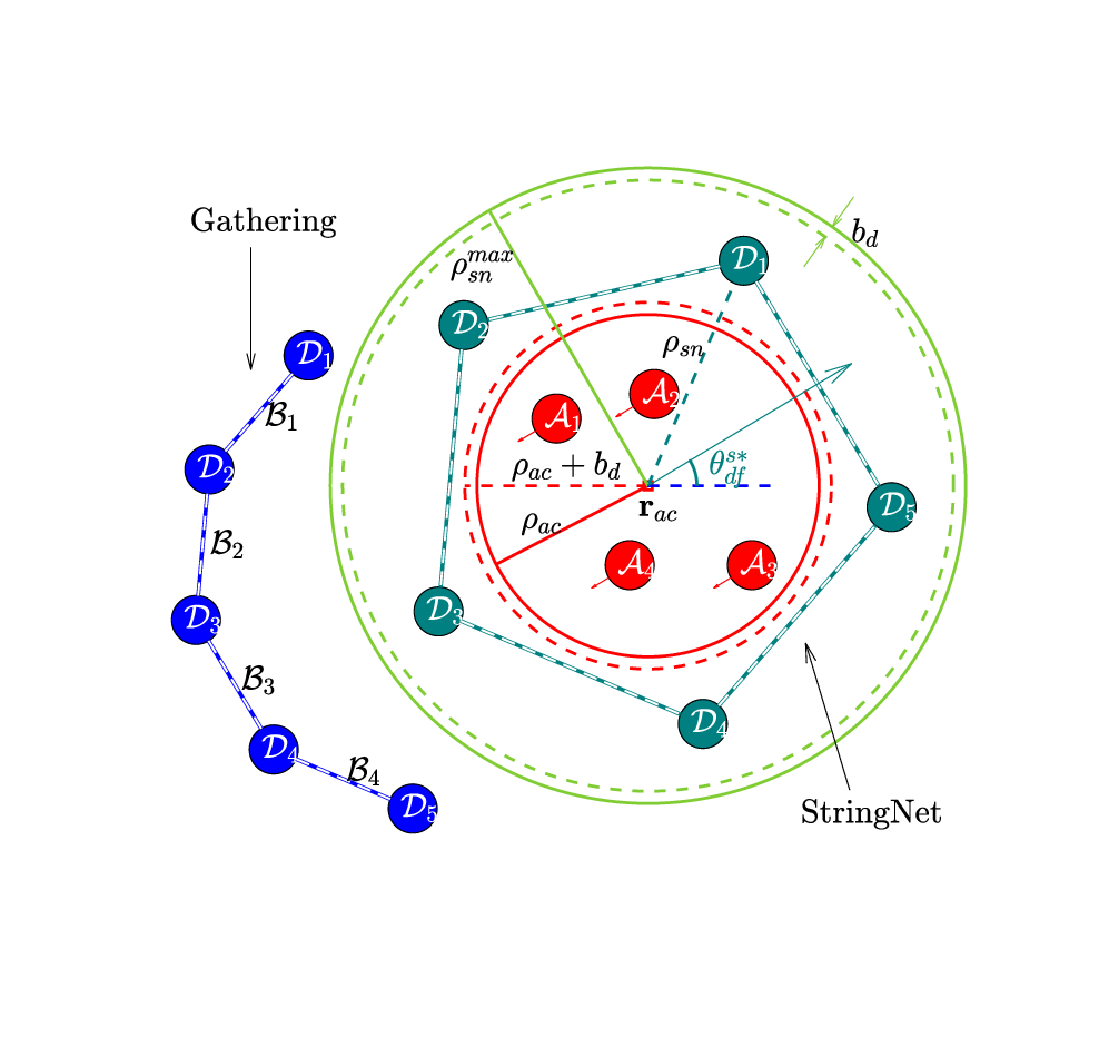
To herd the flock of attackers to $\mathcal{S}$, we propose ‘StringNet Herding’. StringNet is a closed net of strings formed by the defenders as shown in Fig. 2. The strings can be actual physical strings (ropes) or some mechanism that does not allow the attackers to pass through them. It is assumed that even after being connected by the strings, the motion of defenders is not restricted. The underlying graph structure for the ‘StringNet’ is defined as:

The StringNet herding consists of three phases: 1) Gathering, 2) StringNet formation and 3) Herding the StringNet to $\mathcal{S}$. These phases are discussed as follows.

References

- [1] M. Chen, Z. Zhou, and C. J. Tomlin, “Multiplayer reach-avoid games via pairwise outcomes,” IEEE Transactions on Automatic Control, vol. 62, no. 3, pp. 1451–1457, 2017.
- [2] M. Coon and D. Panagou, “Control strategies for multiplayer target-attacker-defender differential games with double integrator dynamics,” in Conference on Decision and Control. IEEE, 2017, pp. 1496–1502.
- [3] S. Gade, A. A. Paranjape, and S.-J. Chung, “Herding a flock of birds approaching an airport using an unmanned aerial vehicle,” in AIAA Guidance, Navigation, and Control Conference, 2015, p. 1540.
- [4] ——, “Robotic herding using wavefront algorithm: Performance and stability,” in AIAA Guidance, Navigation, and Control Conference, 2016, p. 1378.
- [5] A. A. Paranjape, S.-J. Chung, K. Kim, and D. H. Shim, “Robotic herding of a flock of birds using an unmanned aerial vehicle,” IEEE Transactions on Robotics, vol. 34, no. 4, pp. 901–915, 2018.
- [6] A. Pierson and M. Schwager, “Controlling noncooperative herds with robotic herders,” IEEE Transactions on Robotics, vol. 34, no. 2, pp. 517–525, 2018.
- [7] M. A. Haque, A. R. Rahmani, and M. B. Egerstedt, “Biologically inspired confinement of multi-robot systems,” International Journal of Bio-Inspired Computation, vol. 3, no. 4, pp. 213–224, 2011.
- [8] A. Varava, K. Hang, D. Kragic, and F. T. Pokorny, “Herding by caging: a topological approach towards guiding moving agents via mobile robots,” in Proceedings of Robotics: Science and Systems, 2017.
- [9] R. A. Licitra, Z. D. Hutcheson, E. A. Doucette, and W. E. Dixon, “Single agent herding of n-agents: A switched systems approach,” IFAC-PapersOnLine, vol. 50, no. 1, pp. 14 374–14 379, 2017.
- [10] R. A. Licitra, Z. I. Bell, E. A. Doucette, and W. E. Dixon, “Single agent indirect herding of multiple targets: A switched adaptive control approach,” IEEE Control Systems Letters, vol. 2, no. 1, pp. 127–132, 2018.
- [11] P. Deptula, Z. I. Bell, F. M. Zegers, R. A. Licitra, and W. E. Dixon, “Single agent indirect herding via approximate dynamic programming,” in 2018 IEEE Conference on Decision and Control (CDC). IEEE, 2018, pp. 7136–7141.
- [12] V. S. Chipade and D. Panagou, “Herding an adversarial attacker to a safe area for defending safety-critical infrastructure,” arXiv preprint arXiv:1903.06365, 2019.
- [13] C. W. Reynolds, “Flocks, herds and schools: A distributed behavioral model,” in ACM SIGGRAPH computer graphics, vol. 21, no. 4. ACM, 1987, pp. 25–34.
- [14] R. O. S. R. M. Murray and R. Saber, “Flocking with obstacle avoidance: Cooperation with limited information in mobile networks,” in Proceedings of the 42nd IEEE Conference on Decision and Control, vol. 2. Citeseer, 2003, pp. 2022–2028.
- [15] R. Olfati-Saber, “Flocking for multi-agent dynamic systems: Algorithms and theory,” California Inst of Tech Pasadena Control and Dynamical Systems, Tech. Rep., 2004.
- [16] B. Dai and W. Li, “Flocking of multi-agents with arbitrary shape obstacle,” in Proceedings of the 33rd Chinese Control Conference. IEEE, 2014, pp. 1311–1316.
- [17] H. G. Tanner, A. Jadbabaie, and G. J. Pappas, “Flocking in fixed and switching networks,” IEEE Transactions on Automatic control, vol. 52, no. 5, pp. 863–868, 2007.
- [18] D. Panagou, “Motion planning and collision avoidance using navigation vector fields,” in Proc. of the Int. Conf. on Robotics and Automation. IEEE, 2014, pp. 2513–2518.
- [19] M. Deghat, B. D. Anderson, and Z. Lin, “Combined flocking and distance-based shape control of multi-agent formations,” IEEE Transactions on Automatic Control, vol. 61, no. 7, pp. 1824–1837, 2016.
- [20] R. Volpe and P. Khosla, “Manipulator control with superquadric artificial potential functions: Theory and experiments,” IEEE Transactions on Systems, Man, and Cybernetics, vol. 20, no. 6, pp. 1423–1436, 1990.
- [21] S. P. Bhat and D. S. Bernstein, “Geometric homogeneity with applications to finite-time stability,” Mathematics of Control, Signals and Systems, vol. 17, no. 2, pp. 101–127, 2005.
- [22] H. K. Khalil, Nonlinear control. Pearson New York, 2015.