Systematic Opacity Calculations for KilonovaeSystematic Opacity Calculations for Kilonovae–12

We perform systematic atomic calculations for the elements from Fe ($Z=26$) to Ra ($Z=88$). In this paper, we mainly focus on kilonova emission at $t\mathrel{\hbox to0.0pt{\lower 4.0pt\hbox{\hskip 1.0pt$\sim$}\hss}\raise 1.0pt\hbox{$>$}}1$ day after the merger (hereafter $t$ denotes time after the merger). In such timescale, the temperature in the ejecta is $T\mathrel{\hbox to0.0pt{\lower 4.0pt\hbox{\hskip 1.0pt$\sim$}\hss}\raise 1.0pt\hbox{$<$}}20,000$ K, at which typical ionization stages of heavy elements are either neutral, or singly to triply ionized states (I - IV). We calculate atomic energy levels and radiative transitions of these ions using HULLAC (Hebrew University Lawrence Livermore Atomic Code, Bar-Shalom et al. 2001).

Since the calculation methods are same as in Tanaka et al. 2018, we give only a brief overview of the calculations. In the HULLAC code, the orbital functions are derived by solving the single electron Dirac equation with a central-field potential which includes both a nuclear field and a spherically averaged potential due to electron-electron interactions. Then, $N$-electron configuration state functions are constructed by coupled anti-symmetric products of the orbital functions. Relativistic configuration interaction (RCI) calculations are performed with the configuration state functions. In the RCI calculations, we include the ground-state and low excited-state configurations, which have a bulk contribution to the bound-bound opacity. The configurations used in our calculations are summarized in Table 2. The total Hamiltonian consisting of the Dirac-Coulomb Hamitonian, the Breit interaction and the leading QED corretions is diagonalized with the multi configuration state functions, and atomic energy levels are obtained as eigenvalues of the total Hamiltonian. Electric-dipole transition probabilities are calculated in length (Babushkin) gauge.

In the HULLAC code, the central-field potential is constructed from an electron charge distribution of the Slater-type orbital (see Equation (3) of Tanaka et al. 2018), for which we use the ground state configuration of the next higher charge state. The potential is optimized so that the first-order configuration average energies of the ground state and low-lying excited states are minimized. The configurations used for the energy minimization are shown in bold in Table 2. To perform systematic calculations, we normally choose only the ground configuration for the energy minimization. However, we also include other configurations when the lowest energy for each configuration significantly deviates from that in the NIST Atomic Spectra Database (ASD, Kramida et al. 2018).

Since the calculations involve several assumptions as described above, we test the validity of our results by comparing the calculated ionization potential and derived energy levels with those in the NIST ASD. Although some uncertainties exist in the NIST data, this is the best possible way to evaluate our results. We do not include actinide elements because the energy levels are poorly known for most of them.

Figure 1 shows comparison of ionization potentials. Our atomic calculations give reasonable agreement, capturing the trend as a function of atomic number. In general, the agreement in higher ionization states is better, and the results of the neutral atoms shows the largest deviation in particular at high atomic numbers ($Z\mathrel{\hbox to0.0pt{\lower 4.0pt\hbox{\hskip 1.0pt$\sim$}\hss}\raise 1.0pt\hbox{$>$}}60$). The averaged fractional accuracies as compared with the NIST data are 14 %, 7 %, 4 %, and 4% for neutral atoms, singly, doubly, and triply ionized ions, respectively.

Overall agreement in the energy levels is similar to our previous results for selected elements (Tanaka et al. 2018). Some examples of energy levels are shown in Appendix A. Figure 2 shows typical accuracy of the lowest energy level for each configuration. For each configuration, we evaluate the difference in the lowest energy between our calculations and NIST data ($|\Delta E|$). The lower panel shows the median of $|\Delta E|$ normalized by the ionization potential ($E_{\rm pot}$). The number of configuration used for the comparison is shown in the upper panel. As shown in the figure, a typical $|\Delta E|/E_{\rm pot}$ is $<20$ % for neutral and $<10$ % for singly to triply ionized ions (except for $Z\geq 85$, see Section 2.2).

It is important to understand how accuracies in atomic calculations influence the bound-bound opacities. Since the NIST database only includes critically evaluated energy levels, the information of energy levels are not complete, and thus, we cannot compare the accuracies of all the energy levels. Therefore, it is not possible to directly evaluate the impact of the accuracy in atomic calculations to the opacities. Only the possible way is comparing the opacities calculated with different atomic codes or different assumptions in the atomic calculations. Kasen et al. 2013 shows that the difference in the strategy in the atomic calculations results in the difference in the opacity of Nd up to by a factor of 2. Tanaka et al. 2018 and Gaigalas et al. 2019 calculated the bound-bound opacities of selected $r$-process elements by using the HULLAC code and the GRASP2K code (Jönsson et al. 2013), which enables more ab-initio calculations without free parameters. They found that (1) overall wavelength dependence of the bound-bound opacities agree very well, (2) the maximum deviation is about a factor of 2 in ultraviolet wavelengths, and (3) the difference in the Planck mean opacities is up to a factor of 1.5. A similar agreement, within a factor of 1.5-2, is also seen in the opacities of Nd ii calculated by Kasen et al. 2013 and Fontes et al. 2017.

Therefore, we regard that a typical level of systematic uncertainty in the bound-bound opacity is about a factor of 2. As shown in the following sections, the elemental variation of the opacities is much larger than this uncertainty. This means that lack of data for some elements have a bigger impact to the opacity than the accuracy and systematics in the atomic calculations.

Figure 3 summarizes the calculated energy levels for all the elements from $Z=26$ to $Z=88$. The color scale represents the distribution of energy levels, i.e., the number of energy levels in every 0.2 eV energy bin. As expected from complexity measure (Kasen et al. 2013), $f$-shell elements have a larger number of energy levels than the other elements and then $d$-shell and $p$-shell elements follow.

Thanks to the systematic calculations for many elements, we identify the following two effects that mainly determine the energy level distribution. (1) Within a certain electron shell, the distribution of the energy levels tend to be shifted toward higher energy as more electrons occupy the shell (e.g., $Z=40$-$48$ for the case of $4d$ shell and $Z=57$-$71$ for the case of $4f$ shell). Since orbital radii become smaller with $Z$, Coulomb and spin-orbit integrals increase for higher $Z$, or in other words, electron-electron interaction and spin-orbit interaction energies become higher for higher $Z$. Therefore, the energy spacing, i.e., the energy difference to the neighboring level with the same parity and total angular momentum states, also increases along with $Z$ for a particular shell (see Figure 20-2 of Cowan 1981 for the case of $4f$ shell). As a result, the distribution of the energy levels becomes wider for higher $Z$ for a given shell. (2) At the same time, the number of states is the largest for the half-closed shell since it gives the highest complexity, i.e., the number of combinations formed from different quantum numbers is the largest.

The latter effect is strong in lanthanide elements ($Z=57-71$). The total number of levels is the largest for elements around Eu or Gd which have half closed $4f$-shells. But the distribution of the energy levels is pushed up for these elements, and thus, the number of low-lying levels is not necessarily higher than that of other lanthanide elements. This is the reason why the bound-bound opacities of these complex elements are not always higher than those of the other lanthanides (see Section 3). In addition, due to the former effect, the energy distributions of the elements with the conjugate configurations are wider for higher $Z$. For example, Dy I ($Z=66$, with the ground configuration of $4f^{10}6s^{1}$) has a wider energy distribution than the conjugate Nd I ($Z=60$, $4f^{4}6s^{1}$). By this effect, Nd I tends to have higher bound-bound opacities than Dy I, in particular for a low temperature (see Section 3).

In Figure 2, the elements with $Z\geq 85$ show large deviations from the NIST data. For these elements, configuration energies for 6s, 6p and 7s electrons are found to be pushed up because electrons in these orbitals are too much compressed in a small region, and feel a strong electron-electron repulsion. The repulsive interaction is effectively reduced by including configuration mixing with outer orbitals, but the overall energy level distribution tends to be extended to higher energy. Also, by the presence of the strong mixing configuration, the label of the energy level is not clear, which makes direct comparison with the NIST data difficult. Due to these facts, the opacities of these heavy elements can be more uncertain than those of the other elements. We discuss the impact to the opacities in the following sections.

Open $f$-shell elements (lanthanides) have larger opacities than the elements with other outermost electron shells (Kasen et al. 2013; Tanaka & Hotokezaka 2013; Fontes et al. 2017; Tanaka et al. 2018; Wollaeger et al. 2018; Fontes et al. 2020). Due to the large number of energy levels with small energy spacing, the opacities remain high in the NIR wavelengths (left panels of Figure 5). Depending on the elements and temperature, the Planck mean opacities are $\kappa\sim 0.1-50\ {\rm cm^{2}\ g^{-1}}$ (right panels).

For $T=5,000$ K, Planck mean opacities of Pr, Nd, and Pm ($Z=59,60$, and 61) are the highest among lanthanide elements (Figure 6). The opacities gradually decrease as more electrons occupy 4$f$-shell. This is because the number of low-lying energy levels decreases as $f$-shell has more electrons (i.e., $Z$ increases). Although the total number of energy levels is the largest for nearly half-closed $f$-shell elements (Eu or Gd), their opacities are not necessarily highest, as also found by Kasen et al. 2017 and Fontes et al. 2020. This is understood by the relatively high energy level distributions of Eu and Gd (Figure 3).

For $T>10,000$ K, the Planck mean opacities are the highest for nearly half-closed elements (Figure 6). This is because high excited levels of Eu or Gd start to contribute to the opacities. Also, at this temperature, the lanthanides are doubly ionized and low-$Z$ lanthanide elements such as Pr and Nd have smaller contributions to the opacities.

Temperature dependence is different for low and high electron occupations in $f$-shell (Figure 6). This dependence is more clearly visible in the right panels of Figure 5. Low-$Z$ lanthanide elements such as Ce, Pr, Nd ($Z=$ 58, 59, and 60) show decreasing Planck mean opacities as a function of temperature because they have smaller number of electrons in 4$f$-shell. On the other hand, elements with more $f$-shell electrons such as Sm, Eu, Gd, Tb, Dy, Ho, Er, Tm, and Yb ($Z=62-70$) show increasing opacities with temperature since they become closer to half-closed shell as temperature increases.

As shown in the right panels of Figure 5, our opacity data for $f$-shell elements are applicable only at $T\mathrel{\hbox to0.0pt{\lower 4.0pt\hbox{\hskip 1.0pt$\sim$}\hss}\raise 1.0pt\hbox{$<$}}20,000$ K since our atomic calculations include only up to triply ionized ions. This temperature corresponds to about $0.5-1$ day after the merger although this epoch depends on the ejecta parameters such as mass, velocity, and opacity. We need atomic calculations for highly ionized ions to correctly understand the emission at earlier epochs.

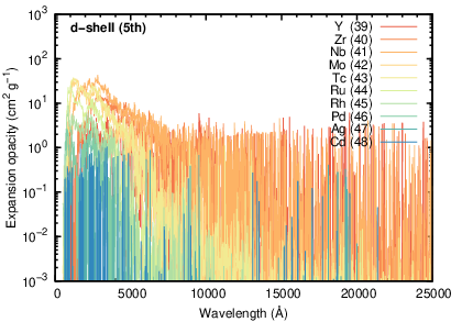
Open $d$-shell elements have the second largest contributions to the opacities after open $f$-shell elements. Compared with the $f$-shell elements, the opacities of the $d$-shell elements have a stronger wavelength dependence, i.e., the opacities are more concentrated to the shorter wavelengths around $1,000-3,000$ Å (left panels of Figure 7). The Planck mean opacities are within the range of $\kappa\sim 0.01-10\ {\rm cm^{2}\ g^{-1}}$ (right panels).

For relatively low temperature ($T<5,000$ K), the elements with a smaller number of $d$-shell electrons tend to have larger opacities (Figure 8). This is due to the lower energy level distributions and larger number of active strong transitions for the elements with the smaller number of $d$-shell electrons (Figure 3). For a higher temperature, the contributions to the opacities from the elements with 1 or 2 electrons in neutral atoms (Zr and Nb for 4$d$, Hf and Ta for 5$d$) becomes smaller (right panels in Figure 7) since these elements do not have $d$-shell electrons when doubly ionized. This is the reason why the Planck mean opacities have a peak around groups 7 and 8 at $T=10,000$ K.

As in the case of $f$-shell elements, opacities are underestimated at a high temperature ($T\mathrel{\hbox to0.0pt{\lower 4.0pt\hbox{\hskip 1.0pt$\sim$}\hss}\raise 1.0pt\hbox{$>$}}20,000$ K) due to the lack of atomic data of higher ionization states. The applicable temperature range for $d$-shell elements is wider than that of $f$-shell elements because of the higher ionization potential of the $d$-shell elements.

Open $p$-shell elements have smaller contributions to the opacities compared with open $d$-shell and $f$-shell elements (Kasen et al. 2013; Tanaka et al. 2018; Wollaeger et al. 2018). The opacities are highest at ultraviolet wavelengths (left panels of Figure 9). For the optical and near-infrared wavelengths, the Planck mean opacities increase as a function of temperature but they are at most $\kappa\sim 1\ {\rm cm^{2}\ g^{-1}}$ for $T<20,000$ K (right panels).

As in the cases for open $d$-shell elements, the opacities of $p$-shell elements are smaller for more $p$-shell electrons (Figure 4) since the distribution of energy levels is shifted toward higher energy. This trend is more significant because the average energy levels of $p$-shell elements are higher than those of $d$-shell elements (Figure 3).

As discussed in Section 2, the elements with $Z\geq 85$ show large deviation in the energy level as compared with the NIST data. The energy levels of these elements tend to be pushed up. As a result, the opacities of these elements are significantly underestimated. At $T<5000$ K, the Planck mean opacity of At ($Z=85$) becomes lower than that of I ($Z=53$) by a factor of 100. The effect is even bigger for Rn ($Z=86$): the opacity of Rn is lower than that of Xe ($Z=54$) by a factor of 100 for a wide temperature range. Therefore, we regard that the opacities of these elements are not reliable. Note that the contribution of these elements to the total opacity in the NS merger ejecta is quite small (see Section 4).

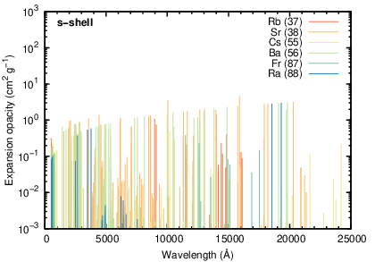
The opacities of open $s$-shell elements are almost negligible to the total opacities. Since there are fewer number of transitions, they do not form quasi-continuum opacities (left panel of Figure 10). For the typical temperature of kilonovae, the Planck mean opacities are $\kappa\mathrel{\hbox to0.0pt{\lower 4.0pt\hbox{\hskip 1.0pt$\sim$}\hss}\raise 1.0pt\hbox{$<$}}0.1\ {\rm cm^{2}\ g^{-1}}$ (right panel). Note that, as for the case of At ($Z=85$) and Rn ($Z=86$), our opacities for Fr ($Z=87$) and Ra ($Z=88$) are not reliable. Although the opacity of Fr shows similar trend with Rb ($Z=37$), the opacity of Ra is significantly lower than those of the other $s$-shell elements.

Overall low opacities of $s$-shell elements do not necessarily mean that they do not contribute to the outcome of kilonova emission. In fact, open $s$-shell elements such as Na, Mg, and Ca often show strong absorption lines in stellar spectra. and thus, $s$-shell elements may contribute to absorption lines in the spectra (see Watson et al. 2019 for the identification of Sr in the spectra of AT2017gfo). Unfortunately, since the atomic calculations for $r$-process elements do not give spectroscopic accuracy, i.e., high enough accuracy to predict the exact wavelengths of each transition, the usefulness of our opacity data for open $s$-shell elements is limited.

Ejecta from NS mergers consist of mixture of $r$-process elements. Abundance distribution is mainly determined by electron fraction $Y_{\rm e}$. The first dynamical ejecta have a wide $Y_{\rm e}$ distribution down to $Y_{\rm e}\sim 0.1$ (Wanajo et al. 2014; Sekiguchi et al. 2015; Sekiguchi et al. 2016; Goriely et al. 2015; Radice et al. 2016; Foucart et al. 2016) while subsequent post-merger ejecta can have higher $Y_{\rm e}$ due to the neutrino absorption if a massive neutron star remains for longer than a certain period (Fernández & Metzger 2013; Fujibayashi et al. 2018; Radice et al. 2018a; Fernández et al. 2019). Lanthanide elements are efficiently produced with $Y_{\rm e}\mathrel{\hbox to0.0pt{\lower 4.0pt\hbox{\hskip 1.0pt$\sim$}\hss}\raise 1.0pt\hbox{$<$}}0.25$ (Lippuner & Roberts 2015; Kasen et al. 2015, e.g., ). Therefore, if the ejecta consists of material with $Y_{\rm e}>0.25$, a short-lived, bright and blue emission is expected due to the absence of high opacity lanthanide (Metzger & Fernández 2014; Kasen et al. 2015; Tanaka et al. 2018; Wollaeger et al. 2018; Miller et al. 2019).

Thanks to the systematic atomic data, we are now able to connect the abundance pattern or electron fraction $Y_{\rm e}$ with the atomic opacities in a more reliable manner. For the mixture of the elements, we construct a line list from Kurucz’s line list (Kurucz & Bell 1995) for $Z=1-28$, the VALD database (Piskunov et al. 1995; Ryabchikova et al. 1997; Kupka et al. 1999; Kupka et al. 2000) for $Z=29$ and 30, and the results of our new atomic calculations for $Z=31-88$.

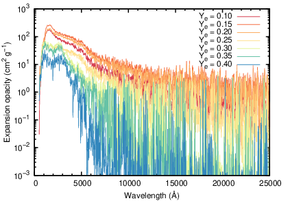
Figure 11 shows expansion opacities for different $Y_{\rm e}$. At $Y_{\rm e}\leq 0.20$, the opacities are dominated by lanthanide elements. The Planck opacities do not strongly depend on $Y_{\rm e}$ and stay around $\kappa\sim 20-30\ {\rm cm^{2}\ g^{-1}}$ at $T>5,000$ K. The temperature dependence at $T>5,000$ K is weaker than in individual elements because of the mixture of the elements with different peaks positions as a function of temperature. Note that the opacities for the case of $Y_{\rm e}=0.10$ may be underestimated due to the lack of actinide elements in our calculations.

These low Ye cases ($Y_{\rm e}=0.10$ and $0.15$) synthesize the heavy elements ($Z\geq 85$) that show the large deviation of the energy levels compared with the NIST data. However, the impact to the opacities is limited. We calculate the opacities for the mixture of the elements by replacing the atomic data for $6p$ and $7s$ elements with those for $5p$ and $6s$ elements, respectively. We confirm that the Planck mean opacities are affected at most by $1\%$ due to these changes. This is reasonable since the mass fractions of these heavy elements are small and the opacities of $s$-shell and $p$-shell elements are subdominant as compared with $f$-shell elements.

The opacities are smaller for higher $Y_{\rm e}$ as relative fractions of lanthanides decrease (Table 1). For $Y_{\rm e}=0.25-0.35$, the Planck mean opacities are dominated by the $d$-shell element (4th period in the periodic table) and they are in the range of $\kappa=1-10\ {\rm cm^{2}\ g^{-1}}$ at $T>5,000$ K. The opacities slightly increase with temperature due to the contribution of latter half of $d$-shell elements (group 8–11, see Figure 8). For $Y_{\rm e}=0.4$, the contributions from $d$-shell elements decrease and the opacities are even lower, i.e., $\kappa=0.1-1\ {\rm cm^{2}\ g^{-1}}$ at $T>5,000$ K.

At a high temperature ($T\mathrel{\hbox to0.0pt{\lower 4.0pt\hbox{\hskip 1.0pt$\sim$}\hss}\raise 1.0pt\hbox{$>$}}20,000$ K), the opacity of the low $Y_{\rm e}$ case decreases more rapidly than that of the high $Y_{\rm e}$ case. This is due to the limitation of ionization states in our atomic data (see Sections 3.1 and 3.2), i.e., our opacity data are not applicable for high temperature. Since the ionization potentials of $d$-shell elements are generally higher than those of $f$-shell elements, the applicable temperature range is wider for high $Y_{\rm e}$ cases, where $d$-shell elements dominate the opacities.

Note that the opacity of $\kappa=0.1-0.5\ {\rm cm^{2}\ g^{-1}}$ is often used for blue kilonovae because it gives a good approximation for Type Ia supernova, where Fe is the major component in the abundance. However, the opacities of mixture of $r$-process elements are almost always higher than $\kappa=0.1-0.5\ {\rm cm^{2}\ g^{-1}}$ even for high $Y_{\rm e}$, except for a low temperature ($T<2,000$ K). This is because Fe is not necessarily representative of $d$-shell elements and the contribution of Fe-like elements (Ru and Os) is low compared with other $d$-shell elements at $T<10,000$ K (Figure 7).

For the ease of applications in analytical models, we give average values of the Planck mean opacities in Table 1. However, it is emphasized that the average opacities are derived only at $T=5,000-10,000$ K and there is a strong temperature dependence at $T<5,000$ K.

The opacities in the NS merger ejecta depend not only on elements and temperature but also the density of the ejecta (and thus, the position in the ejecta). Therefore, the opacities evolves with time by the combination of these effects. In this section, we apply our new atomic data to radiative transfer simulations of kilonovae and study the time variation of the opacities in the ejecta. We use a Monte-Carlo radiative transfer code developed by Tanaka & Hotokezaka 2013; Tanaka et al. 2014 and further updated by Kawaguchi et al. 2018 to include special-relativistic effects. We adopt a simple one-dimensional ejecta model with a power-law density structure $\rho\propto r^{-3}$ from $v=0.05c$ to $v=0.2c$ (Metzger et al. 2010; Metzger 2017), which gives an average velocity of $\langle v\rangle=0.1c$. The total mass is set to be $M_{\rm ej}=0.03M_{\odot}$.

The radiative transfer code adopts nuclear heating rates and abundances of $r$-process elements according to the value of $Y_{\rm e}$. Note that, for relatively high $Y_{\rm e}$, the nuclear heating rate strongly depends on $Y_{\rm e}$ since a few isotopes can dominate the heating rate in a certain timescale. Thus, an assumption of single $Y_{\rm e}$ ejecta, which is not the case in realistic conditions, can lead to misleading results. Therefore, we perform simulations with the following three $Y_{\rm e}$ ranges: high $Y_{\rm e}$ ($Y_{\rm e}=0.30-0.40$, no lanthanide), intermediate $Y_{\rm e}$ ($Y_{\rm e}=0.20-0.30$, lanthanide fraction of $\sim 5\times 10^{-3}$), and low $Y_{\rm e}$ ($Y_{\rm e}=0.10-0.20$, lanthanide fraction of $\sim 0.1$). The heating rate and abundances are averaged over the $Y_{\rm e}$ range above by using single-$Y_{\rm e}$ nucleosynthesis calculations with a step of $\Delta Y_{\rm e}=0.01$ by Wanajo et al. 2014. The thermalization efficiencies of $\gamma$-rays, $\alpha$ particles, $\beta$ particles, and fission are separately taken into account by analytically estimating characteristic timescales (Barnes et al. 2016).

Figure 12 shows the time evolution of Planck mean opacity at $v=0.1c$. It shows the total opacity but the bound-bound opacity is always dominant. From $t=1$ to 10 days, the opacity increases with time for low and intermediate $Y_{\rm e}$ cases, while it slowly decreases for high $Y_{\rm e}$ case. The time evolution of the expansion opacity (Equation (2)) is controled by the competition between the term of $1/\rho t$, which increases with time as $t^{2}$, and the summation of $1-e^{-\tau}$, which generally decreases with time as the lines get weaker for as the density decreases. The decrease of the line strength is more significant in the high $Y_{\rm e}$ case, which results in the temporal decrease of the opacity. Note that even with the increase in the opacity (for the low and intermediate $Y_{\rm e}$ cases), the optical depth of the ejecta, $\tau\sim\kappa\rho R$, decreases. In addition to the overall trend, the opacities shows temporal variation reflecting the temperature evolution, as shown in Figure 11. A significant decrease at $t\sim 10$ days corresponds to the sharp drop of the opacities at low temperature $T<2000$ K.

Overall degree of time variation is about an order of magnitude from $t=1$ to 10 days. This gives a caveat to the use of a constant opacity in the analysis of kilonova light curves, although it is useful to derive physical parameters. Figure 12 also shows a hypothetical case where the abundance of the high $Y_{\rm e}$ model is replaced with Fe. As discussed in Section 4.1, Fe is not a representative element for $d$-shell elements. Therefore, the use of Fe for high $Y_{\rm e}$ opaicty underestimates the opacity by a factor of 2-5 up to $t=2-3$ days and by a factor of more than 10 at later time.

Finally we show the emergent light curves and spectra from the simulations in the previous section. Compared with our previous calculations (Tanaka et al. 2018) using only Se ($p$-shell), Ru ($d$-shell), Te ($p$-shell), Nd ($f$-shell), and Er ($f$-shell) as representative elements, the light curves with new opacity data are more smooth both in time and wavelength. In particular, the use of representative elements can often exaggerate emission in certain wavelengths. At later time ($t\mathrel{\hbox to0.0pt{\lower 4.0pt\hbox{\hskip 1.0pt$\sim$}\hss}\raise 1.0pt\hbox{$>$}}10$ days), only transitions from low-lying energy levels contribute the opacities. And thus, the use of small number of elements artificially enhances contributions from transitions of these elements. These effects are smeared out by properly including all the elements, which results in smooth spectra.

As expected from the properties of the opacities, the bolometric light curve of the model with high $Y_{\rm e}$ has a shorter timescale while that with low $Y_{\rm e}$ has a longer timescale (Figure 13). Compared with the observed luminosity of AT2017gfo associated with GW170817, the early ($t\sim 1-2$ days) light curve are most similar to the high $Y_{\rm e}$ model while the later light curve are most similar to the intermediate $Y_{\rm e}$ model.

These models also give a reasonable agreement with the multi-color light curves of AT2017gfo (Figure 14), although our models are very simple, and ejecta parameters such as mass and velocity are not tuned to reproduce the properties of AT2017gfo. The high $Y_{\rm e}$ model gives the early emission dominated in the optical wavelengths while the intermediate $Y_{\rm e}$ model gives the later emission dominated in the NIR wavelengths. It is emphasized that the optical/NIR flux ratio reflects the wavelength dependence of the opacities, and thus, cannot be accurately predicted by the calculations with a gray opacity.

The low $Y_{\rm e}$ model overproduces the total luminosity and gives too red color, which suggests that such a low $Y_{\rm e}$ component with a lanthanide fraction of $X({\rm La})\sim 0.1$ is not dominant ($M_{\rm ej}\ll 0.03M_{\odot}$). This is consistent with a relatively low lanthanide fraction $X({\rm La})\mathrel{\hbox to0.0pt{\lower 4.0pt\hbox{\hskip 1.0pt$\sim$}\hss}\raise 1.0pt\hbox{$<$}}0.01$ estimated by the spectral and light curve modelling (Chornock et al. 2017; Kasen et al. 2017; Kilpatrick et al. 2017; Tanaka et al. 2017; Tanvir et al. 2017).

The spectral features in our models are of interest because this is the first systematic calculations with the atomic data of the $r$-process elements. Figure 15 compares the model spectra with the observed spectra of GW170817/AT2017gfo with VLT/X-Shooter (Pian et al. 2017; Smartt et al. 2017). The models capture overall spectral shape and its evolution: the high $Y_{\rm e}$ model gives a similar shape of the optical spectra at early phases while intermediate $Y_{\rm e}$ model gives a similar NIR flux level at later phases.

However, detailed spectral features are not necessarily consistent between the observations and models. This is not surprising because our atomic data do not have an enough accuracy for each transition wavelength. To identify the spectral features, we need to use either well-calibrated (but not complete) atomic data as done by Tanaka & Hotokezaka 2013 and Watson et al. 2019 or very accurate atomic calculations as done by Gaigalas et al. 2019 and Radžiūtė et al. 2020.

There are two potentially important drawbacks in our models. One is too narrow spectral features in the early spectra. This is due to the assumption of $\langle v\rangle=0.1c$ in our model. The observed broader features indicate that the line-forming region of the blue component should have $v>0.1c$. In fact, such high velocities of the blue component have been suggested (Kilpatrick et al. 2017; McCully et al. 2017; Nicholl et al. 2017; Shappee et al. 2017, e.g., ). However, it was based on comparison with previous models, which could exaggerate the spectral features by the incompleteness in the atomic data. The comparison with our new model with the complete opacity data securely confirms the necessity of the high velocity for the blue component.

The other is the deficit of the optical flux at $t\mathrel{\hbox to0.0pt{\lower 4.0pt\hbox{\hskip 1.0pt$\sim$}\hss}\raise 1.0pt\hbox{$>$}}5$ days after the merger. It is difficult to keep the optical flux at $t\mathrel{\hbox to0.0pt{\lower 4.0pt\hbox{\hskip 1.0pt$\sim$}\hss}\raise 1.0pt\hbox{$>$}}5$ days because the optical flux in the high $Y_{\rm e}$ model declines too quickly and those in the intermediate and low $Y_{\rm e}$ models are suppressed too much. This difficulty remains even by changing ejecta mass and velocity. We may obtain a better agreement by assuming a lanthanide fraction somewhat lower than that in the intermediate $Y_{\rm e}$ model ($4.8\times 10^{-2}$). Such a relatively small lanthanide fraction is also supported by the modelling of the light curves (Chornock et al. 2017; Kilpatrick et al. 2017; Tanaka et al. 2017). Although such a intermediate lanthanide fraction requires a fine tuning of $Y_{\rm e}$, it can be naturally realized by the mixing in the ejecta as pointed by Metzger et al. 2018. Note that the interplay between multiple ejecta components also influences the light curve at this epoch (Kawaguchi et al. 2018; Kawaguchi et al. 2020). Alternatively, this difficulty might point out the necessity of more advanced radiative transfer calculations by taking into account non-LTE or fluorescence of numerous transitions, which are known to be important in supernovae (Baron et al. 1995; Pinto & Eastman 2000; Mazzali 2000; Dessart & Hillier 2005, e.g., ).