Technical report
Tomographic Reconstruction of Triaxial Strain Fields from Bragg-Edge Neutron Imaging
J.N. Hendriks, A.W.T. Gregg, R.R. Jackson, C.M. Wensrich, A. Wills, A.S. Tremsin, T. Shinohara, V. Luzin, O. Kirstein.
-
Please cite this version:
J.N. Hendriks, A.W.T. Gregg, R.R. Jackson, C.M. Wensrich, A. Wills, A.S. Tremsin, T. Shinohara, V. Luzin, O. Kirstein.. Tomographic Reconstruction of Triaxial Strain Fields from Bragg-Edge Neutron Imaging. Phys. Rev. Materials, 3:113803, Nov 2019. doi: 10.1103/PhysRevMaterials.3.113803.
Abstract
This paper presents a proof-of-concept demonstration of triaxial strain tomography from Bragg-edge neutron imaging within a three-dimensional sample. Bragg-edge neutron transmission can provide high-resolution images of the average through thickness strain within a polycrystalline material. This poses an associated rich tomography problem which seeks to reconstruct the full triaxial strain field from these images. The presented demonstration is an important step towards solving this problem, and towards a technique capable of studying the residual strain and stress within engineering components. A Gaussian process based approach is used that ensures the reconstruction satisfies equilibrium and known boundary conditions. This approach is demonstrated experimentally on a non-trivial steel sample with use of the RADEN instrument at the Japan Proton Accelerator Research Complex. Validation of the reconstruction is provided by comparison with conventional strain scans from the KOWARI constant-wavelength strain diffractometer at the Australian Nuclear Science and Technology Organisation and simulations via finite element analysis.
I Introduction
Bragg-edge neutron transmission techniques provide a means for obtaining lower dimensional (one- or two-dimensional) strain images from higher dimensional (two- or three-dimensional) strain fields within polycrystalline materials Santisteban et al. 2002a; Tremsin et al. 2012. The success of these techniques (Santisteban et al. 2001; Priesmeyer et al. 1999; Tremsin et al. 2008; Ramadhan et al. 2019), and the development of associated instruments (Johnson et al. 1997; Shinohara and Kai 2015; Shinohara et al. 2016; Tremsin et al. 2010; Carlile 1999; Santisteban et al. 2002b; Priesmeyer et al. 1994) and detectors (Santisteban et al. 2002a; Tremsin et al. 2008; Tremsin et al. 2011) has prompted research into the tomographic reconstruction of strain — i.e. strain tomography. This research aims to provide methods analogous to conventional Computed Tomography (CT) whereby the complete triaxial strain distribution within a sample could be reconstructed from a sufficient set of strain images. As the strain field is a tensor, this is a more complex task than conventional scalar CT.
If successfully developed, methods for the tomographic reconstruction of strain fields from these images could be used to study the residual elastic strain and stress within engineered components. Residual stresses are those which remain after applied loads are removed, for example due to heat treatment, or plastic deformation. Residual stresses may have a significant and unintended impact on a component’s effective strength and service life, particularly its fatigue life. A full field analysis of these stress and strains could have a significant impact on several areas of experimental mechanics. In particular, it could be used to study the residual stress within additively manufactured, laser-clad, preened, welded, cast, forged and/or otherwise processed components. This full field analysis would have significant advantages over destructive and semi-destructive techniques ((Prime 2001; Ajovalasit et al. 2002; Jang et al. 2003; Pang et al. 2003; Leggatt et al. 1996)), and be complementary to point-wise x-ray and neutron diffraction methods ((Hauk 1997; Noyan and Cohen 1987; Fitzpatrick and Lodini 2003; Kisi and Howard 2012; Hutchings et al. 2005)).
Strain tomography falls into the class of ‘rich’ tomography problems where the projected strain image is related to an unknown tensor field. The acquisition and analysis of these strain images is described in detail elsewhere (Santisteban et al. 2002a; Santisteban et al. 2001; Santisteban et al. 2002c). Summarising this process: the relative transmission of neutron pulses with known wavelength-intensity spectra through the sample is measured at a pulsed neutron source (e.g. the Japan Proton Accelerator Research Complex (J-PARC) in Japan, ISIS in the United Kingdom, or the Spallation Neutron Source in the USA). For example, current state-of-the-art Micro-Channel Plate detectors (Tremsin et al. 2011) are capable of measuring the transmitted spectra over an array of pixels with a pixel size of . From this data, the position of a given Bragg-edge (a sudden increase in transmitted intensity as a function of wavelength) is observed at each pixel within the array. The relative position of a Bragg-edge provides a measure of strain at each pixel of the form
| (1) |
where is the wavelength at which the Bragg-edge occurs, is the corresponding Bragg-edge wavelength in a stress-free sample, and the following applies:
- 1.
As with all diffraction measurements, only the elastic component of strain is measured.
- 2.
The measured strain is the normal component in the direction of the transmitted neutron beam.
- 3.
The measurement corresponds to a through-thickness average along the path of the corresponding ray.
The strain measured at each pixel can be related to the strain field using the Longitudinal Ray Transform (LRT) (Abbey et al. 2009; Lionheart and Withers 2015). With the inclusion of measurement error this gives a measurement model as
| (2) |
where the LRT geometry is defined in Figure 1 and is the measurement error term, which is assumed to be zero-mean Gaussian with standard deviation . Estimating the strain field given a set of LRT measurements is made more complex as the LRT mapping is non-injective (Lionheart and Withers 2015; Sharafutdinov 1994). This means that if the strain field components are considered independent, then infinitely many fields could produce the same set of measurements. The null space of the LRT poses a significant challenge to the development of methods for strain tomography.
Strain tomography is an emerging field and research has been undertaken by a small number of groups, providing several methods to reconstruct two-dimensional strain fields. With the exception of (Kirkwood et al. 2019) the majority of recent research has been undertaken by our own group. Several special cases have been considered including axisymmetric systems (Abbey et al. 2009; Abbey et al. 2012; Kirkwood et al. 2015; Gregg et al. 2017; Sato et al. 2015; Kirkwood et al. 2019) and granular systems (Wensrich et al. 2016a). More arbitrary strain fields caused by in-situ loadings have been successfully reconstructed by assuming compatibility (Wensrich et al. 2016b; Hendriks et al. 2017). Methods for reconstructing a broader class of strain fields (i.e. residual strains caused by manufacturing processes) have been developed by ensuring the strain field satisfies equilibrium (Gregg et al. 2018; Jidling et al. 2018; Hendriks et al. 2019a). Outside the field of strain tomography, neutron imaging has a range of applications from neutron radiography and tomography of geomaterials (Perfect et al. 2014) to phase and texture imaging using diffraction contrast techniques (Woracek et al. 2018), and Anderson et al. 2009 is a good reference for the interested reader.
Recently, a Gaussian process based approach suitable for modelling and estimating three-dimensional strain fields has been presented for simulated high-energy X-ray measurements (Hendriks et al. 2019b). Here, following the success of this approach, we present a Gaussian process based approach for neutron transmission strain tomography, and provide an experiment proof-of-concept demonstration.
II Reconstruction Approach
The reconstruction approach is modified from the method presented by Hendriks et al. 2019b. This approach models the strain field by a Gaussian process (Rasmussen and Williams 2006 provides a good introduction), and ensures that the reconstructed strain field satisfies the physical properties of equilibrium; this method assumes the sample to be linearly elastic and isotropic (i.e. without texture). Ensuring the strain field satisfies equilibrium is critical as the LRT mapping (2) has a non-trivial null space (Lionheart and Withers 2015) (i.e. without these constraints a unique solution to the inverse problem does not exist). By enforcing equilibrium the null space is reduced to contain only the trivial field, giving a unique solution to the problem (Hendriks et al. 2019a).
Gaussian processes are suitable for the modelling and estimation of spatially correlated phenomena. The use of Gaussian processes to model and estimate strain fields was pioneered in Jidling et al. 2018. By modelling the Airy stress function, a scalar potential field, by a Gaussian process a solution to the two-dimensional stress (and hence strain) could be given that satisfies equilibrium in the absence of body forces. This method can be extended to three dimensions for which the Beltrami stress functions are used instead of the Airy stress function. The Beltrami stress functions consist of six unique potential fields from which a complete solution to the equilibrium equations in three-dimensions can be given (Sadd 2009). These potential fields are each modelled by a Gaussian process allowing a tri-axial strain field satisfying equilibrium to be reconstructed.
In addition to equilibrium, boundary conditions can be included following the work by Hendriks et al. 2019a. Knowledge about unloaded surfaces for which the distribution of applied forces, known as tractions, is known to be zero can be incorporated. This can be done by including artificial measurements of zero traction at points on the surface not subject to an applied load. This provides information about the stress of the form
| (3) |
where is a point on an unloaded surface, is the triaxial stress field, and is the unit vector perpendicular to the surface. Hooke’s law can then be used to relate this information to the strain field, improving the reconstruction near the samples’ boundary.
A detailed description of the method and its implementation is given by Hendriks et al. 2019b. This requires only minor modification to the measurement model, and the inclusion of traction measurements. The measurement model requires a slight modification due to the difference between high-energy x-ray and neutron transmission strain measurements. For high-energy x-ray strain measurements, the measured strain direction, denoted , is almost perpendicular to the ray direction . Whereas, for neutron transmission strain measurements the direction of measured strain is aligned with the ray, and so . Additionally, a large variation in strain measurement uncertainty is observed and therefore the method is modified so that each measurement can be assigned its own standard deviation. In essence this weights the importance of each measurement according to its confidence given by the strain imaging process. Details of these modifications are given in in Appendix A.
In this paper, this approach is used to reconstruct the strain field within an EN26 steel sample from a set of strain images. The sample, load case, and strain image acquisition are described in Section II.1. The resulting strain field is validated by comparison with conventional diffraction strain scans and FEA results, which are described in Section II.2. The reconstructed strain field and a comparison with the validation data is given in Section II.3; potential sources of error are also discussed in this section.
II.1 Sample Design and Strain Imaging
The method is applied to a set of strain images collected on the RADEN energy-resolved-neutron-imaging instrument at J-PARC (Shinohara and Kai 2015; Shinohara et al. 2016) of an EN26 steel (medium carbon, low alloy) sample. The sample consisted of a steel cube with a precision ground hole of diameter along the diagonal. A load was applied by a interference fit, i.e. shrink fit, with a titanium plug. The sample and plug are shown in Figure 2.
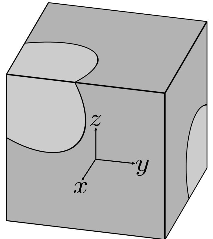


Prior to assembling, the sample was heat treated to relieve stress and provide a uniform tempered-martensite (i.e. ferritic) structure with minimal texture, and with a final hardness of . The sample was assembled by first inserting the plug into a cylinder with an interference fit of , after which a cube with sides was milled from the cylinder and plug.
This sample and loading set-up was designed to provide a smooth three-dimensional strain field suitable for the first demonstration of three-dimensional strain tomography. This has additional advantages for validation as FEA of strain resulting from interference fits is a more straight forward process than FEA of strain fields resulting from plastic deformation.
To this end, a titanium plug was chosen as strain within the plug was ‘invisible’ to the strain imaging process. This is because titanium does not have a Bragg-edge near to the steel Bragg-edge that was chosen for analysis (see Figure 3). As a result, the titanium plug can be ignored during the reconstruction process and considered as imparting an in-situ load on the interior face of the hollow cube.

Strain images were measured using a micro-channel plate detector ( pixels, per pixel)(Tremsin et al. 2011) at a distance of from the source. Each image required hours of beamtime. At the time of the experiment (January 2019) the source power was . Pixels were grouped together into macro pixels of giving sufficient neutron counts to provide a reasonable edge fit; giving a final strain image of macro pixels, each with a resolution of . It is worth noting that this does correspond to the resolution of the final reconstruction and this is discussed more in Section II.3.
Each macro pixel provides a strain measurement of the form (1) where the Bragg-edge position was found following the procedure given by Santisteban et al. 2001 applied to the (110) Bragg-edge. The undeformed location was determined from a stress-free sample. The resulting strain measurements had, on average, an uncertainty of standard deviation . This measurement uncertainty is higher than previously achieved in two-dimensional strain tomography experiments (Hendriks et al. 2017; Gregg et al. 2018). However, further increasing the macro pixel size did not provide a sufficient decrease in uncertainty to warrant the loss in strain image resolution. Additionally, a systematic bias in the edge fit as a function of the measurement path length was observed. This effect was previously described in Vogel 2000 and Gregg et al. 2018; although the exact mechanism is yet to be established. Following Gregg et al. 2018, a linear correction was applied to .
In total 70 strain images were collected. For these images the sample was positioned using a two axis goniometer, which allowed rotation in azimuth and elevation (see Figure 44(a)). Limitations of the experimental set-up restricted the achievable elevation angles to the range from to . Therefore, in order to cover the full range of measurement directions, the sample was repositioned by rotating about the -axis for the final 11 strain images. The measurement directions corresponding to azimuth and elevation angles used are shown in Figure 44(b). Since the LRT is symmetric, measurements with opposite directions provide the same information. Hence, only measurement directions covering one hemisphere are required.


The exact geometry of each neutron ray passing through the sample before reaching the detector is required to model the measurements by the LRT (2). In addition to designing a sample holder to carefully position the sample, an optimisation routine was run to determine the remaining orientation offsets and the offsets between the centre of rotations. The optimisation maximised the sum of Bragg-edge heights associated with rays that would pass through the sample for a given choice of offsets.
Strain fields were reconstructed from this set of strain images using the Gaussian process method described earlier with the inclusion of 400 measurements of zero traction evenly distributed on each of the exterior faces.
II.2 Validation Data
Validation relies on comparison with conventional strain scans (Kisi and Howard 2012; Fitzpatrick and Lodini 2003; Noyan and Cohen 1987) from the KOWARI constant-wavelength strain diffractometer at the Australian Nuclear Science and Technology Organisation (Kirstein et al. 2009; Brule and Kirstein 2006) and Finite Element Analysis (FEA). The strain scans provide measurements of the 6 components of strain on two section planes (33 points on plane 1 and 45 points on plane 2). As with all diffraction methods, these measurements correspond to the average strain inside gauge volumes. These gauge volume locations were chosen on two section planes that were expected to exhibit strong skew symmetry and therefore help to validate a larger region of the reconstruction. The section planes and gauge volume locations are shown in Figure 2.
These measurements were based on the relative shift of the (211) diffraction peak measured with neutrons of wavelength ( geometry) and a gauge volume. The and lattice planes have effectively the same diffraction elastic constants (Daymond and Priesmeyer 2002), therefore the results from the transmission and diffraction experiments can be directly compared without rescaling or recalculation to stress. Sampling times with the KOWARI diffractometer were based on providing uncertainty in strain around : which required 60 hours. The long sampling times required for the comparatively small gauge volumes meant that only a portion of each section plane could be measured.
While only a small amount of the strain field can be verified using the strain scanning measurements, the full reconstructed strain field can be compared to FEA results to provide further validation. Comparison of the reconstruction to the FEA results is made for the three section planes shown in Figure 2.
II.3 Results and Discussion
The reconstructed strain field is shown together with strain scans made on the KOWARI diffractometer and FEA results in Figures 5 and 6. As the KOWARI strain scans cover only a region of section plane 1 and 2, comparison between all three sets is made in these regions only. Example Matlab code to perform this reconstruction and produce the strain plots shown in this paper is available on Github (Hendriks 2019).


Comparison of the KOWARI strain scans, the RADEN reconstruction and the FEA results shows good agreement in general. However, some specific differences can be noted:
- •
In the component of plane 1, the reconstruction shows a region of tension in the bottom right that is also present in the strain scans but is not seen in the FEA.
- •
In the and components of plane 1, the reconstructed strain has the same shape but a greater magnitude than the FEA strain and it is not clear whether this is supported in the strain scans.
- •
In the component of plane 2, the reconstructed strain field has a region of compression also present in the FEA but not seen in the strain scans.
When making these comparison it is important to remember that the KOWARI strain scans are themselves measurements which are relatively noisy ( standard deviation) and are averages over the gauge volumes; this in some cases makes comparison difficult. In particular, the and components of plane 1, and the and components of plane 2 appear particularly noisy.
The FEA strain fields and the reconstructed strain fields are available for the entire sample allowing comparison over the entire section planes 1, 2, and 3; these are shown in Figure 7, Figure 8 and Figure 9 respectively. A selection of strain components is shown for each section plane so that all components are shown at least once. This comparison indicates that the reconstruction shows close agreement with the FEA strain fields on plane 2 and plane 3. The shape of the reconstructed strain field is very similar with the main difference being noted in slightly reduced magnitudes and the peak strains are less concentrated. There is a slightly greater difference between the reconstruction and FEA results observable in plane 1, particularly in the and components. However, at least for the component some of this difference is supported by the KOWARI strain scans which also showed the region of tension present in the bottom right. Additionally, as the strain fields are skew symmetric this would lend some support to the region of tension present in the top left of this component.


From these results, a quantitative assessment of the discrepancies between the the KOWARI strain scan measurements and the reconstruction as well as between the reconstruction and the FEA results was carried out. In both cases the differences are mean zero and Gaussian, implying that there is no systematic error or bias resulting from the reconstruction technique. The differences between the KOWARI strain scans and the reconstruction are calculated by taking gauge volume style averages of the reconstructed strain field and comparing these to the KOWARI measurements. The resulting differences have an average magnitude of . The discrepancies between the FEA and reconstructed strain fields have an average magnitude of .
Although the reconstruction shows, in general, good agreement with the FEA results and KOWARI strain scans some differences have been noted and these differences may be attributed to several sources. Firstly, the number and quality of strain measurements acquired is less than has been previously achieved in two-dimensional strain tomography experiments. In total, 14000 strain measurements were acquired with an average standard deviation of compared to approximately with a standard deviation of in previous two-dimensional experiments (Hendriks et al. 2017; Gregg et al. 2018).
This is in part due to the trade off between macro pixel size and uncertainty in the Bragg-edge fits. While smaller macro pixels ( pixels) would give better resolution in the strain image, the measurement standard deviations would be increased to around . Conversely, larger macro pixels () could be used to decrease the measurement standard deviation to around , however the resolution in the strain image would be made worse. This is in contrast to two-dimensional geometry where the assumption of no out of plane strain variation meant the pixels could be binned into columns without affecting the resolution of the resulting one-dimensional strain image.
It is important to highlight that this measurement uncertainty does not directly correspond to the uncertainty in the reconstructed strain field. Since the reconstruction relies on combining information from multiple strain images, it can have lower uncertainty than the individual strain measurements. A benefit of the Gaussian process method used is that it also gives an estimate of reconstruction’s standard deviation (i.e. the uncertainty in the estimate). For the presented reconstruction, the average standard deviation was , which is marginally better than the neutron diffraction strain measurements used for validation.
Further, the resolution of the strain images, given by the macro pixel size, does not explicitly correspond to the resolution of the reconstruction. Although analogous to conventional CT, the reconstruction method used is fundamentally different. This method does not break the region into discrete voxels, instead it provides a continuous smooth estimate of the strain field where the maximum rate of change is automatically adapted to suit the available data. This means the idea of a reconstruction resolution does not directly apply. Instead, we could look at the maximum strain gradient that can be captured in the reconstruction. For instance, by applying the method to a sample with a step change in strain and analysing the distance over which this change occurs in the reconstruction an equivalent ‘resolution’ could be determined. Since the LRT is only defined within the sample, this step change must be internal, ruling out the application of this idea to our sample. While the reduced peak magnitudes are in part due to the inherent smoothing and as such related to an equivalent resolution, these reductions in magnitude are also due to low certainty in measurements of these regions as a result of small Bragg-edge heights, and macro pixel binning. Hence, an important study for future research would be to apply the method to a sample with an internal step change in strain.
The impact of the binning to form macro pixels is particularly significant in regions near the sample boundary, for example in the corners where the plug and sample intersect. These regions contain a small amount of material and so the averaging effect of the LRT means that the strains are poorly sampled. Additionally, the smaller amount of material means that the Bragg-edge height of any strain measurements passing predominately through these regions is reduced, resulting in poorer measurement confidence. When combined with the macro pixel averaging and inherent smoothing of Gaussian process method, this results in the peak strains in these regions being somewhat obscured. This issue may be somewhat alleviated in future experiments at J-PARC with an expected source power increase to over the next few years.
Differences between reality and the FEA model may also account for some of the observed discrepancies. The sample was milled into a cube from a typical ring and plug. During this process it was not possible to ensure the plug was perfectly on the diagonal of the cube. This would account for the measured strain fields (KOWARI and RADEN) not being entirely skew symmetric and for some of the difference between these fields and the FEA strain field. Additionally, the milling process itself may have introduced residual stresses not accounted for in the FEA model. Finally, the peak stresses are around the yield strength of the material which could result in effects such as hardening and account for differences between the measured strain fields and the FEA strain field.
III Conclusion and Future Work
A proof-of-concept demonstration for triaxial strain reconstruction from neutron transmission strain images has been provided. Strain images were collected using the RADEN energy-resolved-neutron-imaging instrument at J-PARC. The reconstructed strain field was validated by comparison with conventional strain scans from the KOWARI diffractometer and FEA results and shows good agreement.
The reconstruction was performed using a Gaussian process based method that ensures the resulting strain field satisfies equilibrium. This is achieved by using the Beltrami stress functions to provide a complete solution to the stress (and strain) fields in three-dimensions. The reconstruction provides a smooth, continuous estimate of the strain field throughout the entire sample.
The reconstructed strain field was developed within a hollowed EN26 cube by an ‘in-situ’ loading created by interference fitting a titanium plug. Although this strain field is compatible, the method is applicable to a broader class of problems, for example residual strains, as it makes no assumption of compatibility. To this end, future work involves the planning of a three-dimensional residual strain experiment. This could also involve adapting the Gaussian process model to be more suitable for strain fields exhibiting rapid changes or discontinuities.
This is an important step towards the development of strain tomography techniques that can be applied to complex engineered components. While comparison with neutron diffraction measurements was used for validation, we would argue that these methods are complementary rather than opposing. These methods are substantially different; neutron diffraction can measure the average strain within a gauge volume at a specific location, whereas tomography methods attempt to reconstruct the entire strain field. Therefore, we would suggest diffraction measurements are a good choice if a specific region of interest is known, while tomographic methods, such as the one presented in this paper, provide a good alternative if the user wishes to analyse the full field.
Additionally, it was noted that the strain measurements were fewer and of poorer quality than has been previously achieved and that this may have affected the accuracy of the reconstruction. Although this issue may be somewhat alleviated by an increase in source power, future work will also investigate full pattern fitting methods (Luzin et al. 2011; Sato et al. 2013; Sato et al. 2017) which could provide better measurement statistics by analysing multiple Bragg-edges. Full pattern fitting may also provide a path to extending the method to samples that contain significant texture.
Finally, future work should also investigate methods for validating the results when other data sets are not available; such as cross validation (Devijver and Kittler 1982).
Acknowledgements
This work was supported by the Australian Research Council through a Discovery Project Grant No. DP170102324. Access to the RADEN and KOWARI instruments was made possible through the respective user-access programs of J-PARC and ANSTO (J-PARC Long Term Proposal No. 2017L0101 and ANSTO Program Proposal No. PP6050). The authors would also like to thank AINSE Limited for providing financial assistance (PGRA) and support to enable work on this project.
Appendix A Modifications to the Method
This section provides details on the required modifications to the method presented in Hendriks et al. 2019b. This method is modified to adapt the measurement model from one suitable to high-energy X-ray measurements to a model suitable for Bragg-edge neutron transmission measurements, to use individual variances for each each measurement, and to include artificial traction measurements (following Hendriks et al. 2019a). This method models the strain field as a Gaussian process;
| (4) |
where is a vector of the unique components of strain, and is a covariance function designed to ensure all estimated strain fields satisfy equilibrium.
Since both the LRT (2) and the traction measurement model are linear operators, the strain field estimate at location , denoted as , and the measurements are jointly Gaussian;
| (5) |
where and are vectors of all the LRT and traction measurements, respectively. Here, is the variance matrix with the variance of each LRT measurement as an entry on the diagonal, is a small variance placed on the traction measurements for numerical stability, and the required modifications are described in the following.
Within (Hendriks et al. 2019b) the high-energy X-ray strain measurements were modelled using the line integral
| (6) |
which differs from the LRT (2) only in that the measurement direction is a unit vector almost perpendicular to the direction of the ray . Hence the method is easily adapted by substituting , giving the covariance between a strain estimate and the measurement, , as
| (7) |
where ,. The covariance between each pair of measurements, and is similarly given by
| (8) |
Following the work by Hendriks et al. 2019a, a traction measurement can be modelled as
| (9) |
where is a load-free point on the surface with surface normal , and is the stiffness matrix for isotropic materials from Hooke’s law;
| (10) |
Here we will represent the mapping from an estimate of strain to the traction measurement as , which allows the following covariance to be given;
| (11) |
and the covariance between traction measurement and LRT measurement as
| (12) |
Finally, the covariance between a pair of traction measurements and is given by
| (13) |
Once the values for the LRT measurements are known, we can give the strain estimates by using conventional Gaussian conditioning. The rest of the implementation details are the same as those in Hendriks et al. 2019b.
References
- Santisteban et al. (2002a) JR Santisteban, L Edwards, ME Fitzpatrick, A Steuwer, PJ Withers, MR Daymond, MW Johnson, N Rhodes, and EM Schooneveld, “Strain imaging by bragg edge neutron transmission,” Nuclear Instruments and Methods in Physics Research Section A: Accelerators, Spectrometers, Detectors and Associated Equipment 481, 765–768 (2002a).
- Tremsin et al. (2012) AS Tremsin, JB McPhate, A Steuwer, W Kockelmann, A M Paradowska, JF Kelleher, JV Vallerga, OHW Siegmund, and WB Feller, “High-resolution strain mapping through time-of-flight neutron transmission diffraction with a microchannel plate neutron counting detector,” Strain 48, 296–305 (2012).
- Santisteban et al. (2001) JR Santisteban, L Edwards, A Steuwer, and PJ Withers, “Time-of-flight neutron transmission diffraction,” Journal of applied crystallography 34, 289–297 (2001).
- Priesmeyer et al. (1999) Hans Georg Priesmeyer, Meinhard Stalder, Sven Vogel, Kay Meggers, Ralf Bless, and Walter Trela, “Bragg-edge transmission as an additional tool for strain measurements,” Texture, Stress, and Microstructure 33, 173–185 (1999).
- Tremsin et al. (2008) Anton S Tremsin, Jason B McPhate, Winfried A Kockelmann, John V Vallerga, Oswald HW Siegmund, and W Bruce Feller, “Energy-resolving neutron transmission radiography at the isis pulsed spallation source with a high-resolution neutron counting detector,” in 2008 IEEE Nuclear Science Symposium Conference Record (IEEE, 2008) pp. 2902–2908.
- Ramadhan et al. (2019) Ranggi S Ramadhan, Winfried Kockelmann, Triestino Minniti, Bo Chen, David Parfitt, Michael E Fitzpatrick, and Anton S Tremsin, “Characterization and application of Bragg-edge transmission imaging for strain measurement and crystallographic analysis on the IMAT beamline,” Journal of Applied Crystallography 52 (2019).
- Johnson et al. (1997) M.W. Johnson, L. Edwards, and P.J. Withers, “Engin — a new instrument for engineers,” Physica B: Condensed Matter 234-236, 1141 – 1143 (1997), proceedings of the First European Conference on Neutron Scattering.
- Shinohara and Kai (2015) Takenao Shinohara and Tetsuya Kai, “Commissioning start of energy-resolved neutron imaging system, raden in j-parc,” Neutron news 26, 11–14 (2015).
- Shinohara et al. (2016) T Shinohara, T Kai, K Oikawa, M Segawa, M Harada, T Nakatani, M Ooi, K Aizawa, H Sato, T Kamiyama, et al., “Final design of the energy-resolved neutron imaging system “raden” at j-parc,” in Journal of Physics: Conference Series, Vol. 746 (IOP Publishing, 2016) p. 012007.
- Tremsin et al. (2010) A S Tremsin, J B McPhate, J V Vallerga, O H W Siegmund, W B Feller, H Z Bilheux, J J Molaison, C A Tulk, L Crow, R G Cooper, and D Penumadu, “Transmission bragg edge spectroscopy measurements at ORNL spallation neutron source,” Journal of Physics: Conference Series 251, 012069 (2010).
- Carlile (1999) C.J. Carlile, “An instrument suite for the european spallation source,” Physica B: Condensed Matter 266, 131 – 137 (1999).
- Santisteban et al. (2002b) J.R. Santisteban, L. Edwards, H.G. Priesmeyer, and S. Vogel, “Comparison of bragg-edge neutron-transmission spectroscopy at isis and lansce,” Applied Physics A 74, s1616–s1618 (2002b).
- Priesmeyer et al. (1994) Hans Georg Priesmeyer, Kay Meggers, et al., “Neutron diffraction for non-destructive strain/stress measurements in industrial devices,” Journal of Neutron Research 2, 31–52 (1994).
- Tremsin et al. (2011) AS Tremsin, JB McPhate, W Kockelmann, JV Vallerga, OHW Siegmund, and WB Feller, “High resolution Bragg edge transmission spectroscopy at pulsed neutron sources: Proof of principle experiments with a neutron counting MCP detector,” Nuclear Instruments and Methods in Physics Research Section A: Accelerators, Spectrometers, Detectors and Associated Equipment 633, S235–S238 (2011).
- Prime (2001) Michael B Prime, “Cross-sectional mapping of residual stresses by measuring the surface contour after a cut,” Transactions-American society of mechanical engineers journal of engineering materials and technology 123, 162–168 (2001).
- Ajovalasit et al. (2002) A Ajovalasit, Michele Scafidi, Bernardo Zuccarello, M. Beghini, Leonardo Bertini, M. Beghini, Leonardo Bertini, C. Santus, Emilio Valentini, Alessio Benincasa, and Lorenzo Bertelli, Standard test method for determining residual stresses by the hole-drilling strain-gage method,”, ASTM Standard E837 (American Society for Testing and Materials, 2002).
- Jang et al. (2003) Jae-il Jang, Dongil Son, Yun-Hee Lee, Yeol Choi, and Dongil Kwon, “Assessing welding residual stress in a335 p12 steel welds before and after stress-relaxation annealing through instrumented indentation technique,” Scripta Materialia 48, 743–748 (2003).
- Pang et al. (2003) J. W. L. Pang, M Preuss, P. J. Withers, G. J. Baxter, and C Small, “Effects of tooling on the residual stress distribution in an inertia weld,” Materials Science and Engineering: A 356, 405–413 (2003).
- Leggatt et al. (1996) R. H. Leggatt, D. J. Smith, S. D. Smith, and F Faure, “Development and experimental validation of the deep hole method for residual stress measurement,” The Journal of Strain Analysis for Engineering Design 31, 177–186 (1996).
- Hauk (1997) Viktor Hauk, Structural and residual stress analysis by nondestructive methods: Evaluation-Application-Assessment (Elsevier, 1997).
- Noyan and Cohen (1987) Ismail C Noyan and Jerome B Cohen, “Determination of strain and stress fields by diffraction methods,” in Residual Stress (Springer, 1987) pp. 117–163.
- Fitzpatrick and Lodini (2003) Michael E Fitzpatrick and Alain Lodini, Analysis of residual stress by diffraction using neutron and synchrotron radiation (CRC Press, 2003).
- Kisi and Howard (2012) Erich H Kisi and Christopher J Howard, Applications of neutron powder diffraction, Vol. 15 (Oxford University Press, 2012).
- Hutchings et al. (2005) Michael T Hutchings, Philip J Withers, Thomas M Holden, and Torben Lorentzen, Introduction to the characterization of residual stress by neutron diffraction (CRC press, 2005).
- Santisteban et al. (2002c) JR Santisteban, L Edwards, ME Fizpatrick, A Steuwer, and PJ Withers, “Engineering applications of Bragg-edge neutron transmission,” Applied Physics A 74, s1433–s1436 (2002c).
- Abbey et al. (2009) Brian Abbey, Shu Yan Zhang, Wim JJ Vorster, and Alexander M Korsunsky, “Feasibility study of neutron strain tomography,” Procedia Engineering 1, 185–188 (2009).
- Lionheart and Withers (2015) William RB Lionheart and Philip J Withers, “Diffraction tomography of strain,” Inverse Problems 31, 045005 (2015).
- Sharafutdinov (1994) Vladimir A Sharafutdinov, Integral geometry of tensor fields, Vol. 1 (Walter de Gruyter, 1994).
- Kirkwood et al. (2019) HJ Kirkwood, CM Wensrich, AM Paradowska, and B Abbey, “Application and validity of the radon transform applied to axisymmetric neutron strain imaging,” International Journal of Solids and Structures (2019).
- Abbey et al. (2012) Brian Abbey, Shu Yan Zhang, Wim Vorster, and Alexander M Korsunsky, “Reconstruction of axisymmetric strain distributions via neutron strain tomography,” Nuclear Instruments and Methods in Physics Research Section B: Beam Interactions with Materials and Atoms 270, 28–35 (2012).
- Kirkwood et al. (2015) Henry J Kirkwood, Shu Yan Zhang, Anton S Tremsin, Alexander M Korsunsky, Nikolaos Baimpas, and Brian Abbey, “Neutron strain tomography using the radon transform,” Materials Today: Proceedings 2, S414–S423 (2015).
- Gregg et al. (2017) AWT Gregg, JN Hendriks, CM Wensrich, and MH Meylan, “Tomographic reconstruction of residual strain in axisymmetric systems from bragg-edge neutron imaging,” Mechanics Research Communications 85, 96–103 (2017).
- Sato et al. (2015) Hirotaka Sato, Yoshinori Shiota, Takenao Shinohara, Takashi Kamiyama, Masato Ohnuma, Michihiro Furusaka, and Yoshiaki Kiyanagi, “Development of the tensor ct algorithm for strain tomography using bragg-edge neutron transmission,” Physics Procedia 69, 349 – 357 (2015), proceedings of the 10th World Conference on Neutron Radiography (WCNR-10) Grindelwald, Switzerland October 5–10, 2014.
- Wensrich et al. (2016a) Christopher M Wensrich, Johannes Hendriks, and Michael H Meylan, “Bragg edge neutron transmission strain tomography in granular systems,” Strain 52, 80–87 (2016a).
- Wensrich et al. (2016b) CM Wensrich, JN Hendriks, A Gregg, MH Meylan, V Luzin, and AS Tremsin, “Bragg-edge neutron transmission strain tomography for in situ loadings,” Nuclear Instruments and Methods in Physics Research Section B: Beam Interactions with Materials and Atoms 383, 52–58 (2016b).
- Hendriks et al. (2017) JN Hendriks, AWT Gregg, CM Wensrich, AS Tremsin, T Shinohara, M Meylan, EH Kisi, V Luzin, and O Kirsten, “Bragg-edge elastic strain tomography for in situ systems from energy-resolved neutron transmission imaging,” Physical Review Materials 1, 053802 (2017).
- Gregg et al. (2018) AWT Gregg, JN Hendriks, CM Wensrich, Adrian Wills, AS Tremsin, Vladimir Luzin, Takenao Shinohara, Oliver Kirstein, MH Meylan, and EH Kisi, “Tomographic reconstruction of two-dimensional residual strain fields from bragg-edge neutron imaging,” Physical Review Applied 10, 064034 (2018).
- Jidling et al. (2018) Carl Jidling, Johannes Hendriks, Niklas Wahlström, Alexander Gregg, Thomas B. Schön, Christopher Wensrich, and Adrian Wills, “Probabilistic modelling and reconstruction of strain,” Nuclear Instruments and Methods in Physics Research Section B: Beam Interactions with Materials and Atoms 436, 141 – 155 (2018).
- Hendriks et al. (2019a) Johannes Hendriks, Alex Gregg, Chris Wensrich, and Adrian Wills, “Implementation of traction constraints in bragg-edge neutron transmission strain tomography,” Strain 55, e12325 (2019a), e12325 10.1111/str.12325, https://onlinelibrary.wiley.com/doi/pdf/10.1111/str.12325 .
- Perfect et al. (2014) E. Perfect, C.-L. Cheng, M. Kang, H.Z. Bilheux, J.M. Lamanna, M.J. Gragg, and D.M. Wright, “Neutron imaging of hydrogen-rich fluids in geomaterials and engineered porous media: A review,” Earth-Science Reviews 129, 120 – 135 (2014).
- Woracek et al. (2018) Robin Woracek, Javier Santisteban, Anna Fedrigo, and Markus Strobl, “Diffraction in neutron imaging—a review,” Nuclear Instruments and Methods in Physics Research Section A: Accelerators, Spectrometers, Detectors and Associated Equipment 878, 141–158 (2018).
- Anderson et al. (2009) Ian S Anderson, Robert L McGreevy, and Hassina Z Bilheux, “Neutron imaging and applications,” Springer Science+ Business Media, LLC 2209, 987–0 (2009).
- Hendriks et al. (2019b) JN Hendriks, CM Wensrich, and A Wills, “A bayesian approach to triaxial strain tomography from high-energy x-ray diffraction,” arXiv preprint arXiv:1903.02158 (2019b).
- Rasmussen and Williams (2006) Carl Edward Rasmussen and Christopher KI Williams, Gaussian processes for machine learning, Vol. 1 (MIT press Cambridge, 2006).
- Sadd (2009) Martin H Sadd, Elasticity: theory, applications, and numerics (Academic Press, 2009).
- Vogel (2000) Sven Vogel, A Rietveld-Approach for the Analysis of Neutron Time-Of-Flight Transmission Data, Ph.D. thesis, Christian-Albrechts-Universität (2000).
- Kirstein et al. (2009) O Kirstein, V Luzin, and U Garbe, “The strain-scanning diffractometer kowari,” Neutron News 20, 34–36 (2009).
- Brule and Kirstein (2006) Alain Brule and Oliver Kirstein, “Residual stress diffractometer kowari at the australian research reactor opal: status of the project,” Physica B: Condensed Matter 385, 1040–1042 (2006).
- Daymond and Priesmeyer (2002) MR Daymond and HG Priesmeyer, “Elastoplastic deformation of ferritic steel and cementite studied by neutron diffraction and self-consistent modelling,” Acta materialia 50, 1613–1626 (2002).
- Hendriks (2019) J.N. Hendriks, “Three dimensional strain tomography example code,” Github (2019).
- Luzin et al. (2011) V Luzin, K Spencer, and M-X Zhang, “Residual stress and thermo-mechanical properties of cold spray metal coatings,” Acta Materialia 59, 1259–1270 (2011).
- Sato et al. (2013) H Sato, T Shinohara, R Kiyanagi, K Aizawa, M Ooi, M Harada, K Oikawa, F Maekawa, K Iwase, T Kamiyama, et al., “Upgrade of bragg edge analysis techniques of the rits code for crystalline structural information imaging,” Physics Procedia 43, 186–195 (2013).
- Sato et al. (2017) H Sato, K Watanabe, K Kiyokawa, R Kiyanagi, KY Hara, T Kamiyama, M Furusaka, T Shinohara, and Y Kiyanagi, “Further improvement of the rits code for pulsed neutron bragg-edge transmission imaging,” Physics Procedia 88, 322–330 (2017).
- Devijver and Kittler (1982) Pierre A Devijver and Josef Kittler, Pattern recognition: A statistical approach (Prentice hall, 1982).