Explanations can be manipulated
and geometry is to blame

Explanation methods have attracted significant attention over the last years due to their promise to open the black box of deep neural networks. Interpretability is crucial for scientific understanding and safety critical applications.

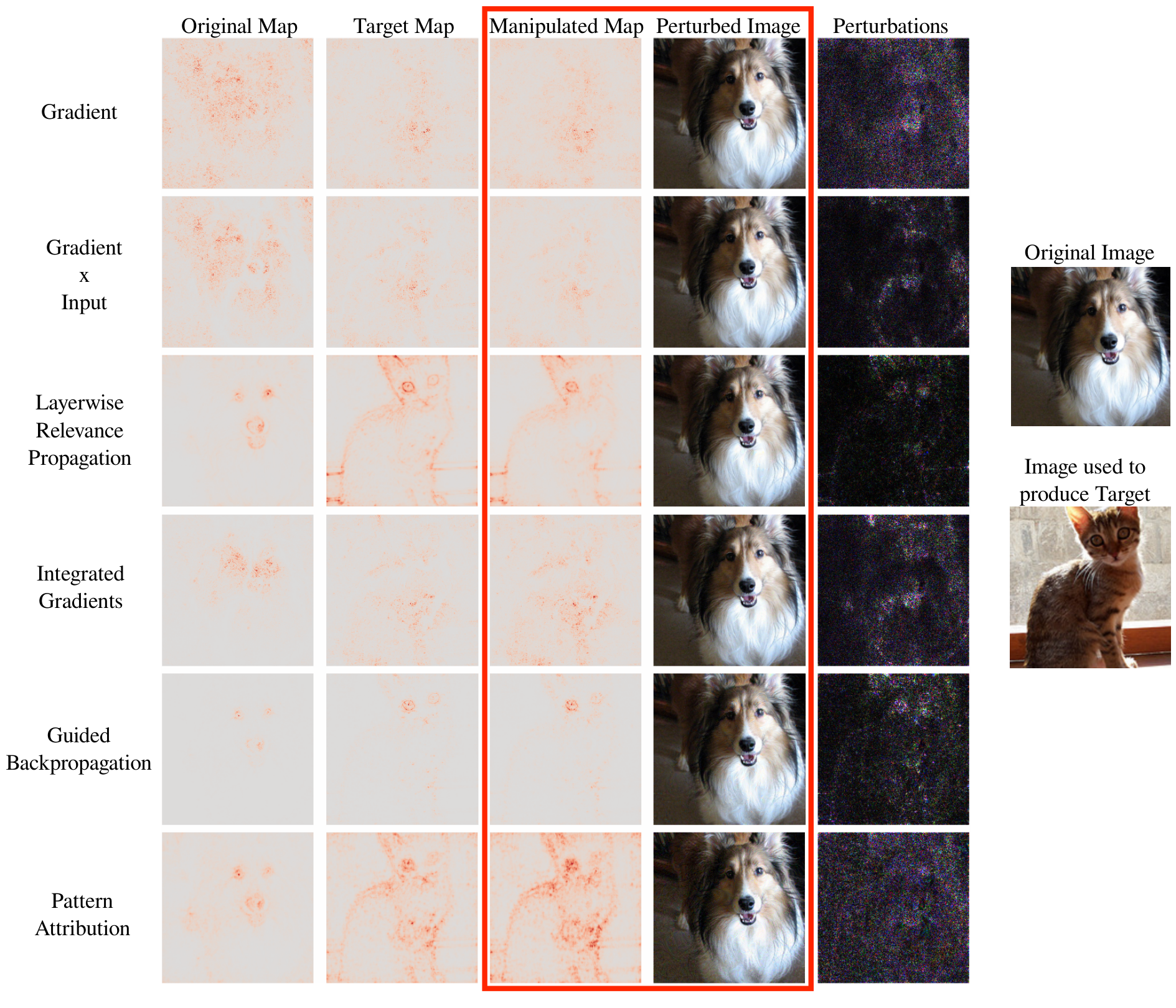
Explanations can be provided in terms of explanation maps[1, 2, 3, 4, 5, 6, 7, 8, 9, 10, 11, 12, 13, 14, 15, 16, 17, 18, 19] that visualize the relevance attributed to each input feature for the overall classification result. In this work, we establish that these explanation maps can be changed to an arbitrary target map. This is done by applying a visually hardly perceptible perturbation to the input. We refer to Figure 1 for an example. This perturbation does not change the output of the neural network, i.e. in addition to the classification result also the vector of all class probabilities is (approximately) the same.

This finding is clearly problematic if a user, say a medical doctor, is expecting a robustly interpretable explanation map to rely on in the clinical decision making process.

Motivated by this unexpected observation, we provide a theoretical analysis that establishes a relation of this phenomenon to the geometry of the neural network’s output manifold. This novel understanding allows us to derive a bound on the degree of possible manipulation of the explanation map. This bound is proportional to two differential geometric quantities: the principle curvatures and the geodesic distance between the original input and its manipulated counterpart. Given this theoretical insight, we propose efficient ways to limit possible manipulations and thus enhance resilience of explanation methods.

In summary, this work provides the following key contributions:

• •

  We propose an algorithm which allows to manipulate an image with a hardly perceptible perturbation such that the explanation matches an arbitrary target map. We demonstrate its effectiveness for six different explanation methods and on four network architectures as well as two datasets.

• •

  We provide a theoretical understanding of this phenomenon for gradient-based methods in terms of differential geometry. We derive a bound on the principle curvatures of the hypersurface of equal network output. This implies a constraint on the maximal change of the explanation map due to small perturbations.

• •

  Using these insights, we propose methods to undo the manipulations and increase the robustness of explanation maps by smoothing the explanation method. We demonstrate experimentally that smoothing leads to increased robustness not only for gradient but also for propagation-based methods.

We consider a neural network $g:\mathbb{R}^{d}\to\mathbb{R}^{K}$ with relu non-linearities which classifies an image $x\in\mathbb{R}^{d}$ in $K$ categories with the predicted class given by $k=\argmax_{i}g(x)_{i}$. The explanation map is denoted by $h:\mathbb{R}^{d}\to\mathbb{R}^{d}$ and associates an image with a vector of the same dimension whose components encode the relevance score of each pixel for the neural network’s prediction. For a given explanation method and specified target $h^{t}\in\mathbb{R}^{d}$, a manipulated image $x_{adv}=x+\delta x$ has the following properties:

1. 1.

   The output of the network stays approximately constant, i.e. $g(x_{adv})\approx g(x)$.

2. 2.

   The explanation is close to the target map, i.e. $h(x_{adv})\approx h^{t}$.

3. 3.

   The norm of the perturbation $\delta x$ added to the input image is small, i.e. $\left\|\delta x\right\|=\left\|x_{adv}-x\right\|\ll 1$ and therefore not perceptible.

Throughout this paper, we will use the following explanation methods:

• •

  Gradient: The map $h(x)=\frac{\partial g}{\partial x}(x)$ is used and quantifies how infinitesimal perturbations in each pixel change the prediction $g(x)$ [2, 1].

• •

  Gradient $\times$ Input: This method uses the map $h(x)=x\odot\frac{\partial g}{\partial x}(x)$ [14]. For linear models, this measure gives the exact contribution of each pixel to the prediction.

• •

  Integrated Gradients: This method defines $h(x)=(x-\bar{x})\odot\int_{0}^{1}\frac{\partial g(\bar{x}+t(x-\bar{x}))}{\partial x}\text{d}t$ where $\bar{x}$ is a suitable baseline. See the original reference [13] for more details.

• •

  Guided Backpropagation (GBP): This method is a variation of the gradient explanation for which negative components of the gradient are set to zero while backpropagating through the non-linearities [4].

• •

  Layer-wise Relevance Propagation (LRP): This method [5, 16] propagates relevance backwards through the network. For the output layer, relevance is defined by¹¹ 1 Here we use the Kronecker symbol $\delta_{i,k}=\begin{cases}1,&\text{for }i=k\\ 0,&\text{for }i\neq k\end{cases}$.

  $\displaystyle R^{L}_{i}=\delta_{i,k}\,,$

  (1)

  which is then propagated backwards through all layers but the first using the $z^{+}$ rule

  $\displaystyle R^{l}_{i}=\sum_{j}\frac{x_{i}^{l}(W^{l})^{+}_{ji}}{\sum_{i}x_{i}^{l}(W^{l})^{+}_{ji}}R^{l+1}_{j}\,,$

  (2)

  where $(W^{l})^{+}$ denotes the positive weights of the $l$-th layer and $x^{l}$ is the activation vector of the $l$-th layer. For the first layer, we use the $z^{\mathcal{B}}$ rule to account for the bounded input domain

  $\displaystyle R^{0}_{i}=\sum_{j}\frac{x_{j}^{0}W^{0}_{ji}-l_{j}(W^{0})^{+}_{ji}-h_{j}(W^{0})^{-}_{ji}}{\sum_{i}(x_{j}^{0}W^{0}_{ji}-l_{j}(W^{0})^{+}_{ji}-h_{j}(W^{0})^{-}_{ji})}R^{1}_{j}\,,$

  (3)

  where $l_{i}$ and $h_{i}$ are the lower and upper bounds of the input domain respectively.

• •

  Pattern Attribution (PA): This method is equivalent to standard backpropagation upon element-wise multiplication of the weights $W^{l}$ with learned patterns $A^{l}$. We refer to the original publication for more details [17].

These methods cover two classes of attribution methods, namely gradient-based and propagation-based explanations, and are frequently used in practice [23, 24].

In this section, we analyze the vulnerability of explanations theoretically. We argue that this phenomenon can be related to the large curvature of the output manifold of the neural network. We focus on the gradient method starting with an intuitive discussion before developing mathematically precise statements.

We have demonstrated that one can drastically change the explanation map while keeping the output of the neural network constant

using only a small perturbation in the input $\delta x$. The perturbed image $x_{adv}=x+\delta x$ therefore lies on the hypersurface of constant network output $S=\{p\in\mathbb{R}^{d}|g(p)=c\}$.⁴⁴ 4 It is sufficient to consider the hypersurface $S$ in a neighbourhood of the unperturbed input $x$. We can exclusively consider the winning class output, i.e. $g(x):=g(x)_{k}$ with $k=\argmax_{i}g(x)_{i}$ because the gradient method only depends on this component of the output. Therefore, the hyperplane $S$ is of co-dimension one. The gradient $\nabla g$ for every $p\in S$ is normal to this hypersurface. The fact that the normal vector $\nabla g$ can be drastically changed by slightly perturbing the input along the hypersurface $S$ suggests that the curvature of $S$ is large.

While the latter statement may seem intuitive, it requires non-trivial concepts of differential geometry to make it precise, in particular the notion of the second fundamental form. We will briefly summarize these concepts in the following (see e.g. [31] for a standard textbook). To this end, it is advantageous to consider a normalized version of the gradient method

This normalization is merely conventional as it does not change the relative importance of any pixel with respect to the others. For any point $p\in S$, we define the tangent space $T_{p}S$ as the vector space spanned by the tangent vectors $\dot{\gamma}(0)=\tfrac{d}{dt}\gamma(t)|_{t=0}$ of all possible curves $\gamma:\mathbb{R}\to S$ with $\gamma(0)=p$. For $u,v\in T_{p}S$, we denote their inner product by $\langle u,v\rangle$. For any $u\in T_{p}S$, the directional derivative is uniquely defined for any choice of $\gamma$ by

We then define the Weingarten map as⁵⁵ 5 The fact that $D_{u}n(p)\in T_{p}S$ follows by taking the directional derivative with respect to $u$ on both sides of $\langle n,n\rangle=1$ .

where the unit normal $n(p)$ can be written as (7). This map quantifies how much the unit normal changes as we infinitesimally move away from $p$ in the direction $u$. The second fundamental form is then given by

It can be shown that the second fundamental form is bilinear and symmetric $\mathcal{L}(u,v)=\mathcal{L}(v,u)$. It is therefore diagonalizable with real eigenvalues $\lambda_{1},\dots\lambda_{d-1}$ which are called principle curvatures.

We have therefore established the remarkable fact that the sensitivity of the gradient map (7) is described by the principle curvatures, a key concept of differential geometry.

In particular, this allows us to derive an upper bound on the maximal change of the gradient map $h(x)=n(x)$ as we move slightly on $S$. To this end, we define the geodesic distance $d_{g}(p,q)$ of two points $p,q\in S$ as the length of the shortest curve on $S$ connecting $p$ and $q$. In the supplement, we show that:

This theorem can intuitively be motivated as follows: for relu non-linearities, the lines of equal network output are piece-wise linear and therefore have kinks, i.e. points of divergent curvature. These relu non-linearities are well approximated by softplus non-linearities (5) with large $\beta$. Reducing $\beta$ smoothes out the kinks and therefore leads to reduced maximal curvature, i.e. $|\lambda_{max}|\leq\beta\,C$. For each point on the geodesic curve connecting $p$ and $p_{0}$, the normal can at worst be affected by the maximal curvature, i.e. the change in explanation is bounded by $|\lambda_{max}|\;d_{g}(p,p_{0})$.

There are two important lessons to be learned from this theorem: the geodesic distance can be substantially greater than the Euclidean distance for curved manifolds. In this case, inputs which are very similar to each other, i.e. the Euclidean distance is small, can have explanations that are drastically different. Secondly, the upper bound is proportional to the $\beta$ parameter of the softplus non-linearity. Therefore, smaller values of $\beta$ provably result in increased robustness with respect to manipulations.

Using the fact that the upper bound of the last section is proportional to the $\beta$ parameter of the softplus non-linearities, we propose $\beta$-smoothing of explanations. This method calculates an explanation using a network for which the relu non-linearities are replaced by softplus with a small $\beta$ parameter to smooth the principle curvatures. The precise value of $\beta$ is a hyperparameter of the method, but we find that a value around one works well in practice.

As shown in the supplement, a relation between SmoothGrad [12] and $\beta$-smoothing can be proven for a one-layer neural network:

Since $p_{\beta}(x)$ closely resembles a normal distribution with variance $\sigma=\log(2)\tfrac{\sqrt{2\pi}}{\beta}$, $\beta$-smoothing can be understood as $N\to\infty$ limit of SmoothGrad $h(x)=\tfrac{1}{N}\sum_{i=1}^{N}\nabla g(x-\epsilon_{i})$ where $\epsilon_{i}\sim g_{\beta}\approx\mathcal{N}(0,\sigma)$. We emphasize that the theorem only holds for a one-layer neural network, but for deeper networks we empirically observe that both lead to visually similar maps as they are considerably less noisy than the gradient map. The theorem therefore suggests that SmoothGrad can similarly be used to smooth the curvatures and can thereby make explanations more robust.⁶⁶ 6 For explanation methods $h(x)$ other than gradient, SmoothGrad needs to be used in a slightly generalized form, i.e. $\tfrac{1}{N}\sum_{i=1}^{N}h(x-\epsilon_{i})$.

Experiments: Figure 4 demonstrates that $\beta$-smoothing allows us to recover the orginal explanation map by lowering the value of the $\beta$ parameter. We stress that this works for all considered methods. We also note that the same effect can be observed using SmoothGrad by successively increasing the standard deviation $\sigma$ of the noise distribution. This further underlines the similarity between the two smoothing methods.

If an attacker knew that smoothing was used to undo the manipulation, they could try to attack the smoothed method directly. However, both $\beta$-smoothing and SmoothGrad are substantially more robust than their non-smoothed counterparts, see Figure 5. It is important to note that $\beta$-smoothing achieves this at considerably lower computational cost: $\beta$-smoothing only requires a single forward and backward pass, while SmoothGrad requires as many as the number of noise samples (typically between 10 to 50).

We refer to Supplement D for more details on these experiments.

Explanation methods have recently become increasingly popular among practitioners. In this contribution we show that dedicated imperceptible manipulations of the input data can yield arbitrary and drastic changes of the explanation map. We demonstrate both qualitatively and quantitatively that explanation maps of many popular explanation methods can be arbitrarily manipulated. Crucially, this can be achieved while keeping the model’s output constant. A novel theoretical analysis reveals that in fact the large curvature of the network’s decision function is one important culprit for this unexpected vulnerability. Using this theoretical insight, we can profoundly increase the resilience to manipulations by smoothing only the explanation process while leaving the model itself unchanged.

Future work will investigate possibilities to modify the training process of neural networks itself such that they can become less vulnerable to manipulations of explanations. Another interesting future direction is to generalize our theoretical analysis from gradient to propagation-based methods. This seems particularly promising because our experiments strongly suggest that similar theoretical findings should also hold for these explanation methods.

References

- [1] David Baehrens, Timon Schroeter, Stefan Harmeling, Motoaki Kawanabe, Katja Hansen, and Klaus-Robert Müller. How to explain individual classification decisions. Journal of Machine Learning Research, 11(Jun):1803–1831, 2010.
- [2] Karen Simonyan, Andrea Vedaldi, and Andrew Zisserman. Deep inside convolutional networks: Visualising image classification models and saliency maps. In 2nd International Conference on Learning Representations, ICLR 2014, Banff, AB, Canada, April 14-16, 2014, Workshop Track Proceedings, 2014.
- [3] Matthew D. Zeiler and Rob Fergus. Visualizing and understanding convolutional networks. In Computer Vision - ECCV 2014 - 13th European Conference, Zurich, Switzerland, September 6-12, 2014, Proceedings, Part I, pages 818–833, 2014.
- [4] Jost Tobias Springenberg, Alexey Dosovitskiy, Thomas Brox, and Martin A. Riedmiller. Striving for simplicity: The all convolutional net. In 3rd International Conference on Learning Representations, ICLR 2015, San Diego, CA, USA, May 7-9, 2015, Workshop Track Proceedings, 2015.
- [5] Sebastian Bach, Alexander Binder, Grégoire Montavon, Frederick Klauschen, Klaus-Robert Müller, and Wojciech Samek. On pixel-wise explanations for non-linear classifier decisions by layer-wise relevance propagation. PloS one, 10(7):e0130140, 2015.
- [6] Ramprasaath R. Selvaraju, Abhishek Das, Ramakrishna Vedantam, Michael Cogswell, Devi Parikh, and Dhruv Batra. Grad-cam: Why did you say that? visual explanations from deep networks via gradient-based localization. CoRR, abs/1610.02391, 2016.
- [7] Marco Tulio Ribeiro, Sameer Singh, and Carlos Guestrin. Why should i trust you?: Explaining the predictions of any classifier. In Proceedings of the 22nd ACM SIGKDD international conference on knowledge discovery and data mining, pages 1135–1144. ACM, 2016.
- [8] Luisa M. Zintgraf, Taco S. Cohen, Tameem Adel, and Max Welling. Visualizing deep neural network decisions: Prediction difference analysis. In 5th International Conference on Learning Representations, ICLR 2017, Toulon, France, April 24-26, 2017, Conference Track Proceedings, 2017.
- [9] Avanti Shrikumar, Peyton Greenside, and Anshul Kundaje. Learning important features through propagating activation differences. In Proceedings of the 34th International Conference on Machine Learning, ICML 2017, Sydney, NSW, Australia, 6-11 August 2017, pages 3145–3153, 2017.
- [10] Scott M Lundberg and Su-In Lee. A unified approach to interpreting model predictions. In I. Guyon, U. V. Luxburg, S. Bengio, H. Wallach, R. Fergus, S. Vishwanathan, and R. Garnett, editors, Advances in Neural Information Processing Systems 30, pages 4765–4774. Curran Associates, Inc., 2017.
- [11] Piotr Dabkowski and Yarin Gal. Real time image saliency for black box classifiers. In I. Guyon, U. V. Luxburg, S. Bengio, H. Wallach, R. Fergus, S. Vishwanathan, and R. Garnett, editors, Advances in Neural Information Processing Systems 30, pages 6967–6976. Curran Associates, Inc., 2017.
- [12] Daniel Smilkov, Nikhil Thorat, Been Kim, Fernanda B. Viégas, and Martin Wattenberg. Smoothgrad: removing noise by adding noise. CoRR, abs/1706.03825, 2017.
- [13] Mukund Sundararajan, Ankur Taly, and Qiqi Yan. Axiomatic attribution for deep networks. In Proceedings of the 34th International Conference on Machine Learning, ICML 2017, Sydney, NSW, Australia, 6-11 August 2017, pages 3319–3328, 2017.
- [14] Avanti Shrikumar, Peyton Greenside, and Anshul Kundaje. Learning important features through propagating activation differences. In Proceedings of the 34th International Conference on Machine Learning, ICML 2017, Sydney, NSW, Australia, 6-11 August 2017, pages 3145–3153, 2017.
- [15] Ruth C Fong and Andrea Vedaldi. Interpretable explanations of black boxes by meaningful perturbation. In 2017 IEEE international conference on computer vision (ICCV), pages 3449–3457. IEEE, 2017.
- [16] Grégoire Montavon, Sebastian Lapuschkin, Alexander Binder, Wojciech Samek, and Klaus-Robert Müller. Explaining nonlinear classification decisions with deep taylor decomposition. Pattern Recognition, 65:211–222, 2017.
- [17] Pieter-Jan Kindermans, Kristof T Schütt, Maximilian Alber, Klaus-Robert Müller, Dumitru Erhan, Been Kim, and Sven Dähne. Learning how to explain neural networks: Patternnet and patternattribution. International Conference on Learning Representations, 2018. https://openreview.net/forum?id=Hkn7CBaTW.
- [18] Been Kim, Martin Wattenberg, Justin Gilmer, Carrie Cai, James Wexler, Fernanda Viegas, and Rory Sayres. Interpretability beyond feature attribution: Quantitative testing with concept activation vectors (tcav). arXiv preprint arXiv:1711.11279, 2017.
- [19] Sebastian Lapuschkin, Stephan Wäldchen, Alexander Binder, Grégoire Montavon, Wojciech Samek, and Klaus-Robert Müller. Unmasking clever hans predictors and assessing what machines really learn. Nature communications, 10(1):1096, 2019.
- [20] Amirata Ghorbani, Abubakar Abid, and James Y. Zou. Interpretation of neural networks is fragile. CoRR, abs/1710.10547, 2017.
- [21] Pieter-Jan Kindermans, Sara Hooker, Julius Adebayo, Maximilian Alber, Kristof T. Schütt, Sven Dähne, Dumitru Erhan, and Been Kim. The (un)reliability of saliency methods. CoRR, abs/1711.00867, 2017.
- [22] Julius Adebayo, Justin Gilmer, Michael Muelly, Ian J. Goodfellow, Moritz Hardt, and Been Kim. Sanity checks for saliency maps. CoRR, abs/1810.03292, 2018.
- [23] Maximilian Alber, Sebastian Lapuschkin, Philipp Seegerer, Miriam Hägele, Kristof T. Schütt, Grégoire Montavon, Wojciech Samek, Klaus-Robert Müller, Sven Dähne, and Pieter-Jan Kindermans. innvestigate neural networks! Journal of Machine Learning Research 20, 2019.
- [24] Marco Ancona, Enea Ceolini, Cengiz Oztireli, and Markus Gross. Towards better understanding of gradient-based attribution methods for deep neural networks. In 6th International Conference on Learning Representations (ICLR 2018), 2018.
- [25] Karen Simonyan and Andrew Zisserman. Very deep convolutional networks for large-scale image recognition. International Conference on Learning Representations, 2014.
- [26] Olga Russakovsky, Jia Deng, Hao Su, Jonathan Krause, Sanjeev Satheesh, Sean Ma, Zhiheng Huang, Andrej Karpathy, Aditya Khosla, Michael Bernstein, Alexander C. Berg, and Li Fei-Fei. ImageNet Large Scale Visual Recognition Challenge. International Journal of Computer Vision (IJCV), 115(3):211–252, 2015.
- [27] Kaiming He, Xiangyu Zhang, Shaoqing Ren, and Jian Sun. Deep residual learning for image recognition. CoRR, abs/1512.03385, 2015.
- [28] Alex Krizhevsky, Ilya Sutskever, and Geoffrey E. Hinton. Imagenet classification with deep convolutional neural networks. In Proceedings of the 25th International Conference on Neural Information Processing Systems - Volume 1, NIPS’12, pages 1097–1105, USA, 2012. Curran Associates Inc.
- [29] Gao Huang, Zhuang Liu, and Kilian Q. Weinberger. Densely connected convolutional networks. CoRR, abs/1608.06993, 2016.
- [30] Alex Krizhevsky. Learning multiple layers of features from tiny images, 2009.
- [31] Loring W Tu. Differential geometry: connections, curvature, and characteristic classes, volume 275. Springer, 2017.
Supplement []
Appendix A Details on experiments
We provide a run_attack.py file in our reference implementation which allows one to produce manipulated images. The hyperparameter choices used in our experiments are summarized in Table 1. We set and for beta growth (see section below for a description). The column ’factors’ summarizes the weighting of the mean squared error of the heatmaps and the images respectively.