跳到论文正文
W Papers独立论文阅读器 arXiv:1906.07957 论文正文 计算阅读时间 · 0%
引用这篇论文根据当前论文元数据生成,正式投稿前建议核对。


License: arXiv.org perpetual non-exclusive license
arXiv:1906.07957v2 [stat.ME] 13 May 2020

Estimation of Markovian-regime-switching models with independent regimes

Nigel Bean Affiliation: School of Mathematical Sciences, The University of Adelaide, Australia Affiliation: Australian Research Council Centre of Excellence in Mathematical and Statistical Frontiers (ACEMS) affiliated authors.    Angus Lewis Thanks: This research was supported by the provision of an Australian Government Research Training Program Scholarship, a University of Adelaide postgraduate research scholarship, and an Australian Research Council Discover Project, Grant/Award Number: ARC DP180103106.
email: angus.lewis@adelaide.edu.au
Affiliation: School of Mathematical Sciences, The University of Adelaide, Australia Affiliation: Australian Research Council Centre of Excellence in Mathematical and Statistical Frontiers (ACEMS) affiliated authors.
   Giang T. Nguyen Affiliation: School of Mathematical Sciences, The University of Adelaide, Australia Affiliation: Australian Research Council Centre of Excellence in Mathematical and Statistical Frontiers (ACEMS) affiliated authors.
Abstract

Markovian-regime-switching (MRS) models are commonly used for modelling economic time series, including electricity prices where independent regime models are used, since they can more accurately and succinctly capture electricity price dynamics than dependent regime MRS models can. We can think of these independent regime MRS models for electricity prices as a collection of independent AR(1) processes, of which only one process is observed at each time; which is observed is determined by a (hidden) Markov chain. Here we develop novel, computationally feasible methods for MRS models with independent regimes including forward, backward and EM algorithms. The key idea is to augment the hidden process with a counter which records the time since the hidden Markov chain last visited each state that corresponding to an AR(1) process.

Keywords: Electricity price model, forward-backward algorithm, hidden Markov model, Markov-switching time series

1 Introduction

A commonly used model for economic time series is the Markovian-regime-switching (MRS) model whereby multiple stochastic processes are interweaved by a Markov chain. The general idea is that there exist multiple regimes underlying the observation process, and depending on which regime the system is in, different characteristics are displayed. For example, for stock prices we could suppose that there is a bull regime where prices trend upward and are comparatively non-volatile, and a bear regime where prices trend downward and are relatively volatile. Our motivating application is electricity prices where it is common to model prices with an MRS model. Due to the fact that electricity cannot currently be stored efficiently, electricity prices show characteristics not seen in typical commodity markets, for example mean reversion, prices spikes, drops and negative prices. MRS models are able to capture these behaviours, and have been popular tools for modelling randomness in electricity markets. Typically MRS models with two or three regimes are used [9, 8, 13, 14]: a base regime where prices are relatively non-volatile, a spike regime where prices are volatile and high, and sometimes a drop regime is included, where prices are volatile and low. More broadly, models with Markovian switching find application in biology [1], weather modelling [23, 27], speech recognition [21] and more.

The earliest applications of MRS models for electricity prices are [9] and [8]. Their models specify that prices decay back to base levels following a spike according to an autoregressive process of order 1 (AR(1)). However, this is not consistent with observations from the market where a more immediate return to base levels is observed [16, 2]. For this reason, [14] introduce a three-regime MRS model which separates the behaviour of base and spike prices. They use one regime to capture base prices, one regime to capture spikes, and one regime to return prices to base levels following a spike. Motivated by the need to capture the distinct and abrupt price spikes in electricity markets, it has become popular to specify MRS models with independent regimes, which are able to capture this behaviour without the addition of the extra regime required by [14]. We may think of a dependent regime MRS models as a single process, where the dynamics of the process is governed by the hidden Markov chain, whereas we may think of an independent regime MRS model as a collection of independent AR(1) processes, and at each time tt, the hidden Markov chain chooses which process is observed.

We say a model has independent regimes if, given the hidden regime sequence, the observations generated from each regime are independent of observations generated from any other regime; and we say a model has dependent regimes otherwise. Independent regime MRS models were introduced in [13] and have since been popular [25, 17, 24]. In these models, typically at least one regime is specified as an AR(1) process. AR(1) processes have a dependence structure between values at successive times which, coupled with the independent regimes assumption in an MRS model, complicates the dependence structure between an observation at time tt and all prior observations – the dependence between prices is governed by the hidden regime process and is therefore random. It is for this reason that the forward, backward and expectation-maximisation (EM) algorithms for traditional (dependent regime) MRS models or hidden Markov models do not apply. For each time tt, the forward algorithm evaluates the probabilities that the hidden process is in each regime given the observed values up to time tt. The backward algorithm then uses the output of the forward algorithm to calculate the probabilities that the hidden process is in each regime given all observations. The EM algorithm is an iterative optimisation algorithm, iterating between an E-step and an M-step, used to find the maximum likelihood estimates of parameters for models with missing data or latent variables – the E-step is computed by the backward algorithm.

For simplicity, in this work, we focus on independent regime MRS models with AR(1) and i.i.d. regimes only, since these are the type of models used in the electricity price modelling literature. However, we believe the methods developed here are more general and apply to Markov-switching processes with regimes that are discrete-time Markov chains generally, and can also be extended to more general autoregressive processes. The most popular method of inference for the models used for electricity pricing is an approximation to the EM algorithm introduced by [17], which we show can be unreliable (see [22] also). Here, a novel, computationally feasible, and exact likelihood-based framework to solve this problem is developed. This work is related to the forward, backward, and EM algorithms for traditional MRS models, and, more closely, to the same algorithms for hidden semi-Markov models, where the idea of augmenting the hidden process with a counter is also used [26]. The novel algorithms have complexity 𝒪⁡(M2​Tk+1​kk)\mathcal{O}\left(M^{2}T^{k+1}k^{k}\right) where M<∞M<\infty is the total number of regimes in the model, TT is the length of the observed data set, and kk is the number of AR(1) regimes in the model. As 𝒪⁡(M2​Tk+1​kk)\mathcal{O}\left(M^{2}T^{k+1}k^{k}\right) may be impractically large depending on the values of TT and kk, we also present an approximation to our algorithm that is 𝒪⁡(M2​T​Dk​kk)\mathcal{O}\left(M^{2}TD^{k}k^{k}\right) where D>0D>0 is the maximum length of the memory of the AR(1) processes, that is, we specify that the observations xtx_{t} may depend only on xt−ℓx_{t-\ell} for ℓ∈{1,2,…,D}\ell\in\{1,2,...,D\}, and is independent of any xt−ℓx_{t-\ell} for ℓ>D\ell>D.

This paper is structured as follows. We formally introduce the MRS model, in particular the independent-regime type in Section 1.1, and discuss the approximate parameter inference algorithm of [17] in Section 1.2. A novel forward algorithm, which is used to evaluate the likelihood and filtered state probabilities for these models, is presented in Section 2. Using the outputs of the forward algorithm we develop a novel backward algorithm in Section 3. The backward algorithm is used to evaluate the smoothed state probabilities, which are applied in Section 4 to construct an EM algorithm. We introduce the truncated approximations of our algorithms at the end of Section 4. Section 5 provides simulation evidence that our EM algorithm is consistent and that the truncation approximations are reasonable, while in Section 6 we apply our algorithms to estimate MRS models for the South Australian wholesale electricity market. Finally, we make concluding remarks in Section 7.

1.1 MRS models: A brief introduction

An MRS model is built from two pieces, an unobservable regime sequence, {Rt}t∈ℕ\{R_{t}\}_{t\in\mathbb{N}}, which is a finite-state Markov Chain, and an observation sequence, {Xt}t∈ℕ\{X_{t}\}_{t\in\mathbb{N}}. Let us denote the state space of the hidden regime sequence as 𝒮={1,2,…,M<∞}\mathcal{S}=\{1,2,\dots,M<\infty\}, and the transition matrix as P=[pi​j]i,j∈𝒮P=[p_{ij}]_{i,j\in\mathcal{S}}.

The simplest MRS model is the hidden Markov model (HMM) where observations XtX_{t} take values in a discrete set, and XtX_{t} is independent of Xt−1,…,X0X_{t-1},\dots,X_{0} and Xt+1,Xt+2,…X_{t+1},X_{t+2},\dots given the regime at time tt, RtR_{t}. In general, MRS models are specified in terms of distributions that allow dependence on past observations, given the current regime. That is, the model defines distributions,

Xt|{Rt,Xt−1,Xt−2,…,X0}∼FRt,X_{t}|\{R_{t},X_{t-1},X_{t-2},\dots,X_{0}\}\sim F^{R_{t}},

for some distribution FRtF^{R_{t}}. The MRS model, as introduced by [10, 11], specifies that Xt|{Rt,Xt−1,Xt−2,…,X0}X_{t}|\{R_{t},X_{t-1},X_{t-2},\dots,X_{0}\} follows some time-series model (an autoregressive process of order pp, for example) with dependence on a finite number of past observations, but not on R0,..,Rt−1R_{0},..,R_{t-1}. That is, the dependence structure does not take into account which regime the past observations belong to. For example, the following is a dependent regime MRS model.

Example 1 (An MRS model with dependent regimes).

Let 𝒮={1,2}\mathcal{S}=\{1,2\}, and p11=p22=0.9p_{11}=p_{22}=0.9, and specify

Xt|{Rt=1,Xt−1,Xt−2,…,X0}=0.6​Xt−1+εt(1),\displaystyle X_{t}|\{R_{t}=1,X_{t-1},X_{t-2},\dots,X_{0}\}=0.6X_{t-1}+\varepsilon_{t}^{\left(1\right)},
Xt|{Rt=2,Xt−1,Xt−2,…,X0}=1+0.9​Xt−1+εt(2).\displaystyle X_{t}|\{R_{t}=2,X_{t-1},X_{t-2},\dots,X_{0}\}=1+0.9X_{t-1}+\varepsilon_{t}^{\left(2\right)}.

for εt(i)∼\varepsilon_{t}^{\left(i\right)}\sim i.i.d. N(0,1) for i=1,2i=1,2. So XtX_{t} follows AR(1) dynamics in both Regimes 1 and 2. This is a dependent-regime MRS model since XtX_{t} depends on Xt−1X_{t-1} regardless of which regime the lagged observation, Xt−1X_{t-1}, came from. Figure 1 (Left) shows a simulation of this model.

Refer to caption
Refer to caption
Figure 1: (Left) Simulation of the dependent regime MRS model example. (Right) Simulation of the independent regime MRS model example. Notice that after a change of regime the independent regime model shows a distinct change in characteristics.

In this paper we relax the assumption that the current observation XtX_{t} is conditionally independent of R0,..,Rt−1R_{0},..,R_{t-1}, in order to increase flexibility in these models. In particular, we consider models where, given Rt=iR_{t}=i, XtX_{t} depends only on lagged values from Regime ii, thus the dependence structure is random as it is a function of R0,…,Rt−1R_{0},\dots,R_{t-1}. The following is an example of an independent regime MRS model.

Example 2 (An MRS model with independent regimes).

Let 𝒮={1,2}\mathcal{S}=\{1,2\}, and p11=p22=0.9p_{11}=p_{22}=0.9, and define the following AR(1) processes

Bt\displaystyle B_{t} =0.6​Bt−1+εtB,\displaystyle=0.6B_{t-1}+\varepsilon_{t}^{B},
St\displaystyle S_{t} =1+0.9​St−1+εtS,\displaystyle=1+0.9S_{t-1}+\varepsilon_{t}^{S},

where εtB\varepsilon_{t}^{B} and εtS\varepsilon_{t}^{S} are sequences of i.i.d. N(0,1) random variables. Then, construct the MRS model as follows

Xt={Bt, if ​Rt=1,St, if ​Rt=2.X_{t}=\begin{cases}B_{t},&\text{ if }R_{t}=1,\\ S_{t},&\text{ if }R_{t}=2.\end{cases}

Figure 1 (Right) shows a simulation of this model.

A precise definition of dependent and independent regime models is the following. Define the sets 𝒜i:={t∈ℕ:Rt=i}\mathcal{A}_{i}:=\{t\in\mathbb{N}:R_{t}=i\}, i∈𝒮i\in\mathcal{S}. We say that a model has independent regimes if, given the regime sequence, the sets {Xt:t∈𝒜i}\{X_{t}:t\in\mathcal{A}_{i}\}, i∈𝒮i\in\mathcal{S}, are independent. Otherwise, it is a dependent regime model.

1.2 Existing methods

For the simplest form of MRS model, the HMM, likelihood evaluation and maximisation algorithms were first developed in a series of papers, [5], [4], and [6], and subsequent work on MRS models is typically closely related to this. The first algorithms for the more general dependent regime MRS model were presented by [10, 11]. The main issue for maximum likelihood estimation of models with hidden regimes is that the regime sequence is unobserved, thus to naively evaluate the likelihood requires calculation of the marginal distribution

L⁡(𝜽):=f𝑿𝜽​(𝒙)=∑𝑹∈𝒮T+1f𝑿,𝑹𝜽​(𝒙,𝑹)=∑𝑹∈𝒮T+1f𝑿|𝑹𝜽​(𝒙|𝑹)​f𝑹𝜽​(𝑹),L\left(\boldsymbol{\theta}\right):=f^{\boldsymbol{\theta}}_{\boldsymbol{X}}\left(\boldsymbol{x}\right)=\sum_{\boldsymbol{R}\in\mathcal{S}^{T+1}}f^{\boldsymbol{\theta}}_{\boldsymbol{X},\boldsymbol{R}}\left(\boldsymbol{x},\boldsymbol{R}\right)=\sum_{\boldsymbol{R}\in\mathcal{S}^{T+1}}f^{\boldsymbol{\theta}}_{\boldsymbol{X}|\boldsymbol{R}}\left(\boldsymbol{x}|\boldsymbol{R}\right)f^{\boldsymbol{\theta}}_{\boldsymbol{R}}\left(\boldsymbol{R}\right), (1)

where f𝒀𝜽​(⋅)f_{\boldsymbol{Y}}^{\boldsymbol{\theta}}\left(\cdot\right) denotes the distribution function of a random vector 𝒀\boldsymbol{Y} with parameters 𝜽\boldsymbol{\theta}, 𝒙=(x0,…,xT)\boldsymbol{x}=\left(x_{0},\dots,x_{T}\right) is a sequence of observed values, and 𝒮T+1\mathcal{S}^{T+1} is the space of all possible regime sequences of length T+1T+1, 𝑹=(R0,…,RT)\boldsymbol{R}=\left(R_{0},...,R_{T}\right). The number of sequences in 𝒮T+1\mathcal{S}^{T+1} is MT+1M^{T+1} which, for most realistic datasets, is computationally infeasible to evaluate in this form. In the context of HMMs, the sum (1) is made computationally feasible by the forward algorithm [6], and the maximisation of the likelihood is commonly performed via the Baum-Welch algorithm [6], which is a specific case of the EM algorithm [7] and uses the backward algorithm [6].

The works of [10, 11] extend the methods for HMMs to MRS models with dependent regimes by adapting the forward algorithm, developing a new algorithm to replace the backward algorithm and constructing an EM algorithm. [20] refines the work of Hamilton, developing a more efficient implementation of Hamilton’s smoothing algorithm. Kim’s algorithm is similar to the backward algorithm for HMMs.

Relevant to this paper, [17] extend Hamilton’s work and develop an approximate algorithm for MRS models with independent regimes, which we label the EM-like algorithm since it resembles Hamilton’s EM algorithm. However, it is not an example of the EM algorithm and so none of the EM theory holds. In Sections 1.2.1–1.2.3, we briefly review the work of [11], [20] and [17] in order to provide the motivation and background for our work.

1.2.1 Likelihood evaluation for dependent-regime models: The forward algorithm

Define 𝒙r:s=(xr,xr+1,…,xs)\boldsymbol{x}_{r:s}=\left(x_{r},x_{r+1},\dots,x_{s}\right) for r≤sr\leq s and write the likelihood as L(𝜽)=fX0𝜽(x0)∏t=1TfXt|𝑿0:t−1𝜽(xt|𝒙0:t−1).L\left(\boldsymbol{\theta}\right)=f^{\boldsymbol{\theta}}_{X_{0}}\left(x_{0}\right)\prod\limits_{t=1}^{T}f^{\boldsymbol{\theta}}_{X_{t}|\boldsymbol{X}_{0:t-1}}\left(x_{t}|\boldsymbol{x}_{0:t-1}\right). The forward algorithm [11] calculates fX0𝜽f^{\boldsymbol{\theta}}_{X_{0}} and f𝜽Xt|𝑿0:t−1f^{\boldsymbol{\theta}}_{X_{t}|\boldsymbol{X}_{0:t-1}} for t=1,2,…,T,t=1,2,\dots,T, from which it is straightforward to calculate the likelihood or loglikelihood:

Algorithm 1: The forward algorithm [11]
  1. Step 1.

    Initialise the algorithm with values ℙ𝜽​(R0=i)=πi\mathbb{P}^{\boldsymbol{\theta}}\left(R_{0}=i\right)=\pi_{i}, which may be assumed to be known a priori, or left as parameters to be inferred.

  2. Step 2.

    The term, fX0𝜽​(x0)f^{\boldsymbol{\theta}}_{X_{0}}\left(x_{0}\right), is calculated as fX0𝜽​(x0)=∑i∈𝒮fX0|R0𝜽​(x0|i)​ℙ𝜽​(R0=i),f^{\boldsymbol{\theta}}_{X_{0}}\left(x_{0}\right)=\sum\limits_{i\in\mathcal{S}}f^{\boldsymbol{\theta}}_{X_{0}|R_{0}}\left(x_{0}|i\right)\mathbb{P}^{\boldsymbol{\theta}}\left(R_{0}=i\right), where the density fX0|R0𝜽f^{\boldsymbol{\theta}}_{X_{0}|R_{0}} is known from the model specification.

  3. Step 3.

    For t=1,…,Tt=1,\dots,T:

    fXt|𝑿0:t−1𝜽(xt|𝒙0:t−1)\displaystyle f^{\boldsymbol{\theta}}_{X_{t}|\boldsymbol{X}_{0:t-1}}\left(x_{t}|\boldsymbol{x}_{0:t-1}\right)
    =∑i∈𝒮fXt|Rt,𝑿0:t−1𝜽(xt|i,𝒙0:t−1)∑j∈𝒮ℙ𝜽(Rt−1=j|𝒙0:t−1)pj​i,\displaystyle\quad=\sum\limits_{i\in\mathcal{S}}f^{\boldsymbol{\theta}}_{X_{t}|R_{t},\boldsymbol{X}_{0:t-1}}\left(x_{t}|i,\boldsymbol{x}_{0:t-1}\right)\sum\limits_{j\in\mathcal{S}}\mathbb{P}^{\boldsymbol{\theta}}\left(R_{t-1}=j|\boldsymbol{x}_{0:t-1}\right)p_{ji},

    where f𝜽Xt|Rt,𝑿0:t−1f^{\boldsymbol{\theta}}_{X_{t}|R_{t},\boldsymbol{X}_{0:t-1}} is also known from the model specification. Furthermore, the probabilities ℙ𝜽(Rt−1=j|𝒙0:t−1)\mathbb{P}^{\boldsymbol{\theta}}\left(R_{t-1}=j|\boldsymbol{x}_{0:t-1}\right) can be calculated using Bayes’ Theorem,

    ℙ𝜽(Rt−1=j|𝒙0:t−1)\displaystyle\mathbb{P}^{\boldsymbol{\theta}}\left(R_{t-1}=j|\boldsymbol{x}_{0:t-1}\right)
    =f𝜽Xt−1|Rt−1,𝑿0:t−2(xt−1|j,𝒙0:t−2)∑i∈𝒮pi​jℙ𝜽(Rt−2=i|𝒙0:t−2)f𝜽Xt−1|𝑿0:t−2(xt−1|𝒙0:t−2),\displaystyle=\cfrac{f^{\boldsymbol{\theta}}_{X_{t-1}|R_{t-1},\boldsymbol{X}_{0:t-2}}\left(x_{t-1}|j,\boldsymbol{x}_{0:t-2}\right)\sum\limits_{i\in\mathcal{S}}p_{ij}\mathbb{P}^{\boldsymbol{\theta}}\left(R_{t-2}=i|\boldsymbol{x}_{0:t-2}\right)}{f^{\boldsymbol{\theta}}_{X_{t-1}|\boldsymbol{X}_{0:t-2}}\left(x_{t-1}|\boldsymbol{x}_{0:t-2}\right)}, (2)

    for t≥2t\geq 2. These are known as the forward/filtered probabilities.

The quantities ℙ𝜽(Rt=i|𝒙0:t−1)=∑j∈𝒮pj​iℙ𝜽(Rt−1=j|𝒙0:t−1)\mathbb{P}^{\boldsymbol{\theta}}\left(R_{t}=i|\boldsymbol{x}_{0:t-1}\right)=\sum\limits_{j\in\mathcal{S}}p_{ji}\mathbb{P}^{\boldsymbol{\theta}}\left(R_{t-1}=j|\boldsymbol{x}_{0:t-1}\right) are known as the prediction probabilities. In some applications, the forward and prediction probabilities may be quantities of interest in their own right, and they also appear as inputs to the backward algorithm (see Section 1.2.2).

1.2.2 Maximum likelihood for dependent-regime models: The EM algorithm

Hamilton’s forward algorithm [11] is a computationally feasible way to evaluate the loglikelihood, from which it is possible to use black-box optimisation methods to find the MLEs. However, it is common to use the EM algorithm [7] instead, particularly when the E-step and M-step of the algorithm are available in closed form. The EM algorithm proceeds by iterating between the E-step, constructing the function Q(𝜽,𝜽n)=𝔼[logf𝑿,𝑹𝜽(𝒙,𝑹)∣𝒙;𝜽n]Q\left(\boldsymbol{\theta},\boldsymbol{\theta}_{n}\right)=\mathbb{E}\left[\log f^{\boldsymbol{\theta}}_{\boldsymbol{X},\boldsymbol{R}}\left(\boldsymbol{x},\boldsymbol{R}\right)\mid\boldsymbol{x};\boldsymbol{\theta}_{n}\right], and the M-step, maximising QQ with respect to 𝜽∈Θ\boldsymbol{\theta}\in\Theta, where Θ\Theta is the parameter space. This results in a sequence {𝜽n}n∈ℕ\{\boldsymbol{\theta}_{n}\}_{n\in\mathbb{N}} that converges to a local maximiser of the loglikelihood.

The EM algorithm for MRS models with dependent regimes proceeds as follows [11]. Define the random variable ηi​j\eta_{ij} as the number of transitions from state ii to state jj in the sequence 𝑹=(R0,…,RT)\boldsymbol{R}=\left(R_{0},\dots,R_{T}\right) and let 𝕀⁡(⋅)\mathbb{I}\left(\cdot\right) be the indicator function. The joint log-density of 𝒙\boldsymbol{x} and 𝑹\boldsymbol{R} can be written as

log⁡f𝑿,𝑹𝜽​(𝒙,𝑹)\displaystyle\log f^{\boldsymbol{\theta}}_{\boldsymbol{X},\boldsymbol{R}}\left(\boldsymbol{x},\boldsymbol{R}\right)
=∑j∈𝒮𝕀⁡(R0=j)​log⁡fX0|R0𝜽​(x0|j)\displaystyle=\sum_{j\in\mathcal{S}}{\mathbb{I}\left(R_{0}=j\right)}\log f^{\boldsymbol{\theta}}_{X_{0}|R_{0}}\left(x_{0}|j\right)
+∑t=1T∑j∈𝒮𝕀(Rt=j)logfXt|Rt,𝑿0:t−1𝜽(xt|j,𝒙0:t−1)\displaystyle\quad{}+\sum_{t=1}^{T}\sum_{j\in\mathcal{S}}{\mathbb{I}\left(R_{t}=j\right)}\log f^{\boldsymbol{\theta}}_{X_{t}|R_{t},\boldsymbol{X}_{0:t-1}}\left(x_{t}|j,\boldsymbol{x}_{0:t-1}\right)
+∑i,j∈𝒮ηi​jlogpi​j+∑j∈𝒮𝕀(R0=j)logπj,\displaystyle\quad{}+\sum_{i,j\in\mathcal{S}}{\eta_{ij}}\log p_{ij}+\sum_{j\in\mathcal{S}}\mathbb{I}\left(R_{0}=j\right)\log\pi_{j},

where πj\pi_{j} denotes ℙθ​(R0=i)\mathbb{P}^{\theta}\left(R_{0}=i\right). In the nnth iteration, n≥0n\geq 0, for the E-step, taking the conditional expectation given parameters 𝜽n\boldsymbol{\theta}_{n} and observed values 𝒙0:T\boldsymbol{x}_{0:T} yields

Q⁡(𝜽,𝜽n)\displaystyle Q\left(\boldsymbol{\theta},\boldsymbol{\theta}_{n}\right) =∑j∈𝒮ℙ𝜽n(R0=j|𝒙0:T)logfX0|R0𝜽(x0|j)\displaystyle=\sum_{j\in\mathcal{S}}{\mathbb{P}^{\boldsymbol{\theta}_{n}}\left(R_{0}=j|\boldsymbol{x}_{0:T}\right)}\log f^{\boldsymbol{\theta}}_{X_{0}|R_{0}}\left(x_{0}|j\right)
+∑t=1T∑j∈𝒮ℙ𝜽n(Rt=j|𝒙0:T)logfXt|Rt,𝑿0:t−1𝜽(xt|j,𝒙0:t−1)\displaystyle\quad{}+\sum_{t=1}^{T}\sum_{j\in\mathcal{S}}{\mathbb{P}^{\boldsymbol{\theta}_{n}}\left(R_{t}=j|\boldsymbol{x}_{0:T}\right)}\log f^{\boldsymbol{\theta}}_{X_{t}|R_{t},\boldsymbol{X}_{0:t-1}}\left(x_{t}|j,\boldsymbol{x}_{0:t-1}\right)
+∑i,j∈𝒮𝔼[ηi​j|𝒙0:T;𝜽n]logpi​j+∑j∈𝒮ℙ𝜽n(R0=j|𝒙0:T)logπj,\displaystyle\qquad+\sum_{i,j\in\mathcal{S}}{\mathbb{E}[\eta_{ij}|\boldsymbol{x}_{0:T};{\boldsymbol{\theta}_{n}}]}\log p_{ij}+\sum_{j\in\mathcal{S}}\mathbb{P}^{\boldsymbol{\theta}_{n}}\left(R_{0}=j|\boldsymbol{x}_{0:T}\right)\log\pi_{j},

where the expectation 𝔼[ηi​j|𝒙0:T;𝜽n]=∑t=1Tℙ𝜽n(Rt=j,Rt−1=i|𝒙0:T)\mathbb{E}[\eta_{ij}|\boldsymbol{x}_{0:T};\boldsymbol{\theta}_{n}]=\sum\limits_{t=1}^{T}\mathbb{P}^{\boldsymbol{\theta}_{n}}\left(R_{t}=j,R_{t-1}=i|\boldsymbol{x}_{0:T}\right). The densities fX0|R0𝜽f^{\boldsymbol{\theta}}_{X_{0}|R_{0}} and f𝜽Xt|Rt,𝑿0:t−1f^{\boldsymbol{\theta}}_{X_{t}|R_{t},\boldsymbol{X}_{0:t-1}}, are given by the model specification.

The smoothed probabilities, ℙ𝜽n(Rt=j|𝒙0:T)\mathbb{P}^{\boldsymbol{\theta}_{n}}\left(R_{t}=j|\boldsymbol{x}_{0:T}\right) and ℙ𝜽n(Rt=j,Rt−1=i∣𝒙0:T)\mathbb{P}^{\boldsymbol{\theta}_{n}}\left(R_{t}=j,R_{t-1}=i\mid\boldsymbol{x}_{0:T}\right), required to construct QQ are obtained using a backward recursion after running the forward algorithm with parameters 𝜽n\boldsymbol{\theta}_{n}, and storing the forward and prediction probabilities. Developed by [20], this backward recursion is in Algorithm 2, below.

Algorithm 2: The backward algorithm [20]
  1. Step 1.

    Evaluate ℙ𝜽n(RT=j|𝒙0:T)\mathbb{P}^{\boldsymbol{\theta}_{n}}\left(R_{T}=j|\boldsymbol{x}_{0:T}\right) using the forward algorithm (Algorithm 1).

  2. Step 2.

    For t=T−1,…,0,t=T-1,\dots,0,

    ℙ𝜽n(Rt=j,Rt+1=i|𝒙0:T)\displaystyle\mathbb{P}^{\boldsymbol{\theta}_{n}}\left(R_{t}=j,R_{t+1}=i|\boldsymbol{x}_{0:T}\right) =pj​i(n)ℙ𝜽n(Rt=j|𝒙0:t)ℙ𝜽n(Rt+1=i|𝒙0:T)ℙ𝜽n(Rt+1=i|𝒙0:t),\displaystyle=p_{ji}^{\left(n\right)}\cfrac{\mathbb{P}^{\boldsymbol{\theta}_{n}}\left(R_{t}=j|\boldsymbol{x}_{0:t}\right)\mathbb{P}^{\boldsymbol{\theta}_{n}}\left(R_{t+1}=i|\boldsymbol{x}_{0:T}\right)}{\mathbb{P}^{\boldsymbol{\theta}_{n}}\left(R_{t+1}=i|\boldsymbol{x}_{0:t}\right)},
    ℙ𝜽n(Rt=j|𝒙0:T)\displaystyle\mathbb{P}^{\boldsymbol{\theta}_{n}}\left(R_{t}=j|\boldsymbol{x}_{0:T}\right) =∑i∈𝒮ℙ𝜽n(Rt=j,Rt+1=i|𝒙0:T),\displaystyle=\sum_{i\in\mathcal{S}}\mathbb{P}^{\boldsymbol{\theta}_{n}}\left(R_{t}=j,R_{t+1}=i|\boldsymbol{x}_{0:T}\right),

    where pi​j(n)p_{ij}^{\left(n\right)} means the pi​jp_{ij} parameter under 𝜽n\boldsymbol{\theta}_{n}.

After executing Kim’s backward algorithm, we can construct the function QQ. In the M-step, the maximisers of Q⁡(⋅,𝜽n)Q\left(\cdot,\boldsymbol{\theta}_{n}\right) are found. In the dependent regime model, if the process is in Regime jj at time tt, then the observations evolve according to Xt=αj+ϕj​Xt−1+σj​εtX_{t}=\alpha_{j}+\phi_{j}X_{t-1}+\sigma_{j}\varepsilon_{t} where αj,\alpha_{j}, ϕj\phi_{j} and σj\sigma_{j} are parameters, and {εt}∼N​(0,1)\{\varepsilon_{t}\}\sim\mbox{N}\left(0,1\right). Recall that, for the dependent regime model, Xt−1X_{t-1} is the last observed value (regardless of which regime generated it). The maximiser of QQ at the (n+1)\left(n+1\right)th iteration of the EM algorithm, 𝜽n+1\boldsymbol{\theta}^{n+1}, for n≥0n\geq 0, is the following system of equations [11, 17]:

ϕj(n+1)\displaystyle\phi^{\left(n+1\right)}_{j} =∑t=1Tℙ𝜽n(Rt=j|𝒙0:T)xt−1B1,t(i)∑t=1Tℙ𝜽n(Rt=j|𝒙0:T)xt−1B2,t(i),\displaystyle=\cfrac{\sum\limits_{t=1}^{T}\mathbb{P}^{\boldsymbol{\theta}_{n}}\left(R_{t}=j|\boldsymbol{x}_{0:T}\right)x_{t-1}B_{1,t}^{\left(i\right)}}{\sum\limits_{t=1}^{T}\mathbb{P}^{\boldsymbol{\theta}_{n}}\left(R_{t}=j|\boldsymbol{x}_{0:T}\right)x_{t-1}B_{2,t}^{\left(i\right)}},
αj(n+1)\displaystyle\alpha^{\left(n+1\right)}_{j} =∑t=1Tℙ𝜽n(Rt=j|𝒙0:T)(xt−ϕ(n+1)jxt−1)∑t=1Tℙ𝜽n(Rt=j|𝒙0:T),\displaystyle=\cfrac{\sum\limits_{t=1}^{T}\mathbb{P}^{\boldsymbol{\theta}_{n}}\left(R_{t}=j|\boldsymbol{x}_{0:T}\right)\left(x_{t}-\phi^{\left(n+1\right)}_{j}x_{t-1}\right)}{\sum\limits_{t=1}^{T}\mathbb{P}^{\boldsymbol{\theta}_{n}}\left(R_{t}=j|\boldsymbol{x}_{0:T}\right)},
(σj2)(n+1)\displaystyle\left(\sigma^{2}_{j}\right)^{\left(n+1\right)} =∑t=1Tℙ𝜽n(Rt=j|𝒙0:T)(xt−α(n+1)j−ϕ(n+1)jxt−1)2∑t=1Tℙ𝜽n(Rt=j|𝒙0:T),\displaystyle=\cfrac{\sum\limits_{t=1}^{T}\mathbb{P}^{\boldsymbol{\theta}_{n}}\left(R_{t}=j|\boldsymbol{x}_{0:T}\right)\left(x_{t}-\alpha^{\left(n+1\right)}_{j}-\phi^{\left(n+1\right)}_{j}x_{t-1}\right)^{2}}{\sum\limits_{t=1}^{T}\mathbb{P}^{\boldsymbol{\theta}_{n}}\left(R_{t}=j|\boldsymbol{x}_{0:T}\right)},\qquad
where
B1,t(i)\displaystyle B_{1,t}^{\left(i\right)} =xt−xt−1−∑s=1Tℙ𝜽n(Rs=j|𝒙0:T)(xs−xs−1)∑s=1Tℙ𝜽n(Rs=j|𝒙0:T),\displaystyle=x_{t}-x_{t-1}-\cfrac{\sum\limits_{s=1}^{T}\mathbb{P}^{\boldsymbol{\theta}_{n}}\left(R_{s}=j|\boldsymbol{x}_{0:T}\right)\left(x_{s}-x_{s-1}\right)}{\sum\limits_{s=1}^{T}\mathbb{P}^{\boldsymbol{\theta}_{n}}\left(R_{s}=j|\boldsymbol{x}_{0:T}\right)},\quad
and B2,t(i)\displaystyle\mbox{ and }\quad B_{2,t}^{\left(i\right)} =∑s=1Tℙ𝜽n(Rs=j|𝒙0:T)xs−1∑s=1Tℙ𝜽n(Rs=j|𝒙0:T)−xt−1.\displaystyle=\cfrac{\sum\limits_{s=1}^{T}\mathbb{P}^{\boldsymbol{\theta}_{n}}\left(R_{s}=j|\boldsymbol{x}_{0:T}\right)x_{s-1}}{\sum\limits_{s=1}^{T}\mathbb{P}^{\boldsymbol{\theta}_{n}}\left(R_{s}=j|\boldsymbol{x}_{0:T}\right)}-x_{t-1}.

In general, the switching probabilities are updated using the following [20]

pi​j(n+1)=∑t=1Tℙ𝜽n(Rt=j|𝒙0:T)pi​j(n)ℙ𝜽n(Rt−1=i|𝒙0:t−1)ℙ𝜽n(Rt=j|𝒙0:t−1)∑t=1Tℙ𝜽n(Rt−1=i|𝒙0:T),\displaystyle p_{ij}^{\left(n+1\right)}=\cfrac{\sum\limits_{t=1}^{T}\mathbb{P}^{\boldsymbol{\theta}_{n}}\left(R_{t}=j|\boldsymbol{x}_{0:T}\right)\cfrac{p_{ij}^{\left(n\right)}\mathbb{P}^{\boldsymbol{\theta}_{n}}\left(R_{t-1}=i|\boldsymbol{x}_{0:t-1}\right)}{\mathbb{P}^{\boldsymbol{\theta}_{n}}\left(R_{t}=j|\boldsymbol{x}_{0:t-1}\right)}}{\sum\limits_{t=1}^{T}\mathbb{P}^{\boldsymbol{\theta}_{n}}\left(R_{t-1}=i|\boldsymbol{x}_{0:T}\right)}, (3)

which rely on the smoothed, forward and prediction probabilities. For i.i.d. regimes the M-step can often be derived analytically; however, such expressions are not required for our discussion since there is no dependence on lagged values in these regimes and so they are omitted.

Thus, we implement the EM algorithm by initialising it with a guess of the true parameters, then alternating between the forward and backward algorithms (the E-step) and calculating the maximisers of QQ (the M-step). The algorithm terminates when the step size is below a prespecified tolerance, i.e. |𝜽n+1−𝜽n|∞<e|\boldsymbol{\theta}_{n+1}-\boldsymbol{\theta}_{n}|_{\infty}<e where ee is some small tolerance.

1.2.3 Approximate maximum likelihood for independent-regime models: The EM-like algorithm

For independent-regime MRS models the EM algorithm is computationally infeasible if the densities f𝜽Xt|Rt,𝑿0:t−1f^{\boldsymbol{\theta}}_{X_{t}|R_{t},\boldsymbol{X}_{0:t-1}}, Rt∈𝒮R_{t}\in\mathcal{S}, t=1,…,Tt=1,\dots,T, are computed naively, as this is a 𝒪⁡(Mt)\mathcal{O}\left(M^{t}\right) calculation for each t=1,…,Tt=1,...,T, where M<∞M<\infty is the number of regimes in the model. On the other hand, if we use our proposed foward algorithm, introduced in Section 2), calculation of these densities is 𝒪⁡(tk+1)\mathcal{O}\left(t^{k+1}\right) for each t=1,…,Tt=1,...,T, which may be computationally feasible when TT and kk are not too large.

Developed by [17], the EM-like algorithm is an approximation to the EM algorithm. For independent regime MRS models, the EM-like algorithm overcomes the problem of computational infeasibility by replacing lagged values for Regime ii (assuming this is an AR(1) regime) with approximations, b~t−1,i(n)\tilde{b}_{t-1,i}^{\left(n\right)}. These are described as the expectations [17], 𝔼[Bti|𝒙0:t;𝜽n],\mathbb{E}[B^{i}_{t}|\boldsymbol{x}_{0:t};\boldsymbol{\theta}_{n}], where

Bti:=𝕀⁡(Rt=i)​xt+𝕀⁡(Rt≠i)​(αi+ϕi​Bt−1i+σi​εti).B_{t}^{i}:=\mathbb{I}\left(R_{t}=i\right)x_{t}+\mathbb{I}\left(R_{t}\neq i\right)\left(\alpha_{i}+\phi_{i}B_{t-1}^{i}+\sigma_{i}\varepsilon_{t}^{i}\right).

Simply put, wherever xt−1x_{t-1} appears verbatim in an expression related to Regime ii in the EM algorithm in Sections 1.2.1-1.2.2, it is replaced with b~t−1,i(n)\tilde{b}_{t-1,i}^{\left(n\right)} at the nthn^{\text{th}} iteration. The b~t,i(n)\tilde{b}_{t,i}^{\left(n\right)} are calculated recursively as

b~t,i(n)\displaystyle\tilde{b}_{t,i}^{\left(n\right)} =ℙ~𝜽n(Rt=i|𝒙0:t)xt+ℙ~𝜽n(Rt≠i|𝒙0:t−1)(αi+ϕib~t−1,i(n)),\displaystyle=\tilde{\mathbb{P}}^{\boldsymbol{\theta}_{n}}\left(R_{t}=i|\boldsymbol{x}_{0:t}\right)x_{t}+\tilde{\mathbb{P}}^{\boldsymbol{\theta}_{n}}\left(R_{t}\neq i|\boldsymbol{x}_{0:t-1}\right)\left(\alpha_{i}+\phi_{i}\tilde{b}_{t-1,i}^{\left(n\right)}\right), (4)

where ℙ~𝜽n(Rt=i|𝒙0:t)\tilde{\mathbb{P}}^{\boldsymbol{\theta}_{n}}\left(R_{t}=i|\boldsymbol{x}_{0:t}\right) and ℙ~𝜽n(Rt≠i|𝒙0:t)\tilde{\mathbb{P}}^{\boldsymbol{\theta}_{n}}\left(R_{t}\neq i|\boldsymbol{x}_{0:t}\right) are given by the forward algorithm which is part of the EM-like procedure. Janczura and Weron, [17], conduct simulation studies and show that this algorithm seems to work well for the datasets they generate. However, no theoretical results are available that show convergence of, or error bounds for, the EM-like algorithm; in particular, there is no guarantee that the parameter estimates produced by the EM-like algorithm are consistent. In contrasts, our algorithms rest on the theory of the EM algorithm.

We can construct examples of independent-regime MRS models where the EM-like algorithm fails to get close to the true parameter values.

Example 3.

Consider the following independent-regime MRS model,

Xt={Bt, if ​Rt=1,Yt, if ​Rt=2,\displaystyle X_{t}=\begin{cases}B_{t},&\text{ if }R_{t}=1,\\ Y_{t},&\text{ if }R_{t}=2,\end{cases} (5)

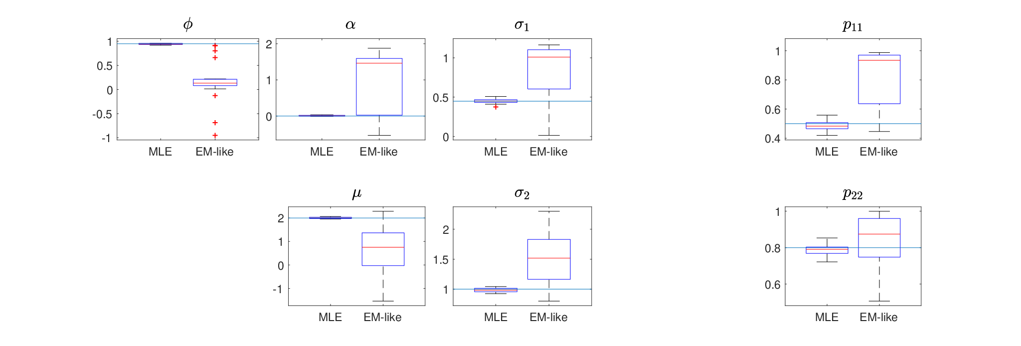
where BtB_{t} is an AR(1) process, Bt=0.95​Bt−1+0.2​εt,B_{t}=0.95B_{t-1}+\sqrt{0.2}\varepsilon_{t}, with {εt}\{\varepsilon_{t}\} being a sequence of i.i.d. N(0,1)\left(0,1\right) random variables, YtY_{t} is an i.i.d. sequence of N(2,1)\left(2,1\right) random variables, and {Rt}t∈ℕ\{R_{t}\}_{t\in\mathbb{N}} is a Markov chain with state space 𝒮={1,2}\mathcal{S}=\{1,2\}, transition matrix entries p11=0.5p_{11}=0.5 and p22=0.8p_{22}=0.8, and initial probability distribution (1,0)\left(1,0\right), so the process always starts in Regime 1. We simulated 20 realisations of length T=2000T=2000 from this model and used the EM-like algorithm to try to recover the true parameters. To give the algorithm the best chance of converging to the true parameters, we initialise the EM-like algorithm at the true parameter values. The parameters recovered by the EM-like algorithm are summarised in Figure 2.
Refer to caption
Figure 2: Boxplots of the parameters recovered by the EM-like algorithm (Right) and the MLEs recovered by our EM algorithm (Left) for Example 3. The blue line represents the true parameter value. Notice that the EM-like algorithm is not able to recover the parameters, while the EM algorithm performs relatively well.

For comparison, the MLEs obtained using our EM algorithm (Section 4) are also shown. Notice in Figure 2 that the EM-like algorithm performs poorly, while our exact method performs much better.

2 A novel forward algorithm

The general idea of the novel algorithms presented in this paper is to augment the hidden Markov chain with counters that record the last time each AR(1) regime was visited. This augmented process is a Markov chain, and similar arguments to those used to construct the forward-backward algorithm for MRS models with dependent regimes can be used to construct a forward and backward algorithms for these models. Our methods are related to the forward and backward algorithms for hidden semi-Markov models, where the hidden process is also augmented with a counter and the augmented hidden process is a Markov chain [26]. Though similar, the algorithms for hidden semi-Markov models (HSMMs) are not applicable to the models considered here since for HSMMs the counter counts the number of time steps since the last change of regime, whereas here the counters count the number of transitions since the last visit to a regime. Furthermore, in HSMMs, the counters do not appear in the conditional densities of the observations, as they do here.

2.1 The augmented hidden Markov chain

For the following, suppose that the first kk states, 𝒮A​R={1,…,k<M}\mathcal{S}_{AR}=\{1,\dotsc,k<M\}, correspond to AR(1) processes and all other regimes are i.i.d. That is, we have the following independent regime MRS model

Xt={Bt1,if ​Rt=1,Btk,if ​Rt=k,Stk+1,if ​Rt=k+1,StM,if ​Rt=M,X_{t}=\begin{cases}B_{t}^{1},&\mbox{if }R_{t}=1,\\ \vdots&\\ B_{t}^{k},&\mbox{if }R_{t}=k,\\ S_{t}^{k+1},&\mbox{if }R_{t}=k+1,\\ \vdots&\\ S_{t}^{M},&\mbox{if }R_{t}=M,\\ \end{cases}

where Bti=αi+ϕi​Bt−1i+σi​εtiB_{t}^{i}=\alpha_{i}+\phi_{i}B^{i}_{t-1}+\sigma_{i}\varepsilon_{t}^{i} are AR(1) and StjS_{t}^{j} are i.i.d. Our arguments also hold for k=Mk=M with only slight modification, but here we treat the case k<Mk<M only, since these are the types of models relevant to our application.

Now, define another Markov chain

{𝑯t}t∈ℕ:={(𝑵t,Rt)}t∈ℕ={(Nt,1,…,Nt,k,Rt)}t∈ℕ,\{\boldsymbol{H}_{t}\}_{t\in\mathbb{N}}:=\{\left(\boldsymbol{N}_{t},R_{t}\right)\}_{t\in\mathbb{N}}=\{\left(N_{t,1},\dotsc,N_{t,k},R_{t}\right)\}_{t\in\mathbb{N}},

where Nt,j∈ℕ+N_{t,j}\in\mathbb{N}_{+} counts the number of time steps since the process {Rt}\{R_{t}\} was last in Regime jj before time tt, for each AR(1) regime j=1,…,kj=1,\dots,k. When there is no time τ∈{0,1,…,t−1}\tau\in\{0,1,\dots,t-1\} with Rτ=jR_{\tau}=j, then we set Nt,j=t+1N_{t,j}=t+1. Thus the augmented Markov chain {𝑯t}t∈ℕ\{\boldsymbol{H}_{t}\}_{t\in\mathbb{N}} lives on the state space ℕ+k×𝒮.\mathbb{N}_{+}^{k}\times\mathcal{S}.

To describe the transitions of the Markov chain {𝑯t}\{\boldsymbol{H}_{t}\}, let 𝒏:=(n1,…,nk)∈ℕ+k\boldsymbol{n}:=\left(n_{1},\dots,n_{k}\right)\in~\mathbb{N}_{+}^{k} be an arbitrary vector of counters, with nr≠nsn_{r}\neq n_{s} for r≠sr\neq s or, at time tt, nr=ns=t+1n_{r}=n_{s}=t+1 (it is possible that neither state rr nor state ss have been visited by time tt). Also, define 𝟏\boldsymbol{1} to be a row vector of ones of length kk, 𝒆i\boldsymbol{e}_{i} to be a row vector of length kk with all entries being 0 except the ithi^{\text{th}} entry which is 1, and 𝒏(−i):=𝒏−ni​𝒆i=(n1,…,ni−1,0,ni+1,…,nk).\boldsymbol{n}^{\left(-i\right)}:=\boldsymbol{n}-n_{i}\boldsymbol{e}_{i}=\left(n_{1},\dots,n_{i-1},0,n_{i+1},\dots,n_{k}\right).

The transition probabilities of {𝑯t}\{\boldsymbol{H}_{t}\} are

ℙ𝜽​(𝑯t+1=(𝒏t+1,j)|𝑯t=(𝒏t,i))\displaystyle\mathbb{P}^{\boldsymbol{\theta}}\left(\boldsymbol{H}_{t+1}=\left(\boldsymbol{n}_{t+1},j\right)|\boldsymbol{H}_{t}=\left(\boldsymbol{n}_{t},i\right)\right)
={pi​jfor i∈𝒮A​Rc,j∈𝒮,𝒏t+1=𝒏t+𝟏,pi​jfor i∈𝒮A​R,j∈𝒮,𝒏t+1=𝒏(−i)t+𝟏,0otherwise.\displaystyle\quad{}=\begin{cases}p_{ij}&\text{for }i\in\mathcal{S}_{AR}^{c},j\in\mathcal{S},\boldsymbol{n}_{t+1}=\boldsymbol{n}_{t}+\boldsymbol{1},\\ p_{ij}&\text{for }i\in\mathcal{S}_{AR},j\in\mathcal{S},\boldsymbol{n}_{t+1}=\boldsymbol{n}^{\left(-i\right)}_{t}+\boldsymbol{1},\\ 0&\text{otherwise}.\end{cases} (6)

In words, when the current state is 𝑯t=(𝒏t,i)\boldsymbol{H}_{t}=\left(\boldsymbol{n}_{t},i\right) and ii is not an AR(1) regime (so there is no counter associated with state ii), then, at time t+1{t+1}, RtR_{t} transitions to state jj with probability pi​jp_{ij} and all the counters are advanced by 11 to 𝒏t+1=𝒏t+𝟏\boldsymbol{n}_{t+1}=\boldsymbol{n}_{t}+\boldsymbol{1}, since there has been one more time step since {Rt}\{R_{t}\} was last in any state with a counter (any state in 𝒮A​R\mathcal{S}_{AR}). When the current state is 𝑯t=(𝒏t,i)\boldsymbol{H}_{t}=\left(\boldsymbol{n}_{t},i\right), where ii is an AR(1) regime, then RtR_{t} transitions to any state j∈𝒮j\in\mathcal{S} with probability pi​jp_{ij}, the counter for Regime ii, nt+1,in_{{t+1},i}, is set to 1, since the last time in state ii was tt, and all other counters are advanced by 11. All other transition probabilities for {𝑯t}\{\boldsymbol{H}_{t}\} are 0.

The state space of {𝑯t}\{\boldsymbol{H}_{t}\} is countably infinite. However, due to the way {𝑯t}t∈ℕ\{\boldsymbol{H}_{t}\}_{t\in\mathbb{N}} is initialised and evolves, many states are inaccessible for {𝑯t}\{\boldsymbol{H}_{t}\}, t∈{0,1,…,T<∞}t\in\{0,1,\dots,T<\infty\}, and this makes our algorithm computationally feasible. Specifically, we suppose that the Markov chain {𝑯t}\{\boldsymbol{H}_{t}\} is initialised with the probability distribution

ℙ⁡(𝑯0=(n0,1,…,n0,k,j))={πj,for j∈𝒮, n0,i=1, for all i∈𝒮A​R,0,otherwise.\displaystyle\mathbb{P}\left(\boldsymbol{H}_{0}=\left(n_{0,1},\dots,n_{0,k},j\right)\right)=\begin{cases}\pi_{j},&\text{for }j\in\mathcal{S},\text{ }n_{0,i}=1,\text{ for all }i\in\mathcal{S}_{AR},\\ 0,&\text{otherwise}.\end{cases} (7)

The distribution 𝝅:=(π1,…,πM)\boldsymbol{\pi}:=\left(\pi_{1},\dots,\pi_{M}\right) can be any proper probability distribution. However, in line with existing algorithms for dependent regime MRS models, it can be either the stationary distribution of {Rt}\{R_{t}\}, or a point mass on a single state, or, when used as part of the EM algorithm, the probabilities ℙ𝜽n(𝑯0|𝒙0:T)\mathbb{P}^{\boldsymbol{\theta}_{n}}\left(\boldsymbol{H}_{0}|\boldsymbol{x}_{0:T}\right) calculated at the previous iteration of the EM algorithm. The following lemma gives all the states that {𝑯t}\{\boldsymbol{H}_{t}\} can be in at time t>0t>0.

Lemma 4.

Define 𝒮(0):={𝟏}\mathcal{S}^{\left(0\right)}:=\{\boldsymbol{1}\} as a vector of 11’s of length kk where kk is the number of AR(1) regimes. For each t=1,2,…,Tt=1,2,\dots,T, let 𝒮(t)\mathcal{S}^{\left(t\right)} be the set of all vectors 𝐧t:=(nt,1,…,nt,k)\boldsymbol{n}_{t}:=\left(n_{t,1},\dots,n_{t,k}\right) such that, for j,m∈𝒮A​Rj,m\in\mathcal{S}_{AR},

  1. (i)

    nt,j∈{1,2,…,t+1}n_{t,j}\in\{1,2,\dots,t+1\},

  2. (ii)

    there are at most min⁡(t,k)\min\left(t,k\right) elements of 𝒏t\boldsymbol{n}_{t} with nt,j≠t+1n_{t,j}\neq t+1,

  3. (iii)

    nt,j≠nt,mn_{t,j}\neq n_{t,m} for all j≠mj\neq m, unless nt,j=nt,m=t+1n_{t,j}=n_{t,m}=t+1.

Given {𝐇t}\{\boldsymbol{H}_{t}\} is initialised with the distribution in Equation (7), it is possible for 𝐇t\boldsymbol{H}_{t} to reach states (𝐧t,i)\left(\boldsymbol{n}_{t},i\right) where 𝐧t∈𝒮(t)\boldsymbol{n}_{t}\in\mathcal{S}^{\left(t\right)} and i∈𝒮i\in\mathcal{S} only. The cardinality of 𝒮(t)\mathcal{S}^{\left(t\right)} is |𝒮(t)|=∑m=0min⁡(t,k)(tm)​(km)​m!.|\mathcal{S}^{\left(t\right)}|=\sum\limits_{m=0}^{\min\left(t,k\right)}\binom{t}{m}\binom{k}{m}m!.

Proof.

First, we explain why 𝒮(t)\mathcal{S}^{\left(t\right)} contains all possible values of the counters of 𝑯t\boldsymbol{H}_{t} for t≥0t\geq 0.

At time t=0t=0 the chain, {𝑯t}={(𝑵t,Rt)}\{\boldsymbol{H}_{t}\}=\{\left(\boldsymbol{N}_{t},R_{t}\right)\}, is initialised with the distribution in Equation (7), so 𝒮(0):={𝟏}.\mathcal{S}^{\left(0\right)}:=\{\boldsymbol{1}\}.

At time t>0t>0, either {Rt}\{R_{t}\} has never visited state j∈𝒮A​Rj\in\mathcal{S}_{AR}, in which case nt,j=t+1n_{t,j}=t+1, or {Rt}\{R_{t}\} last visited jj at time tjt_{j}, in which case nt,j=t−tj∈{1,2,…,t}n_{t,j}=t-t_{j}\in\{1,2,\dots,t\}; this is part (i). Since the process {Rt}\{R_{t}\} can only be in one regime at a time, it follows that nt,j≠nt,mn_{t,j}\neq n_{t,m} for j≠mj\neq m (unless nt,j=nt,m=t+1n_{t,j}=n_{t,m}=t+1), which is part (iii) of the definition. Also, at time tt, the regime chain {Rt}\{R_{t}\} could only possibly have visited min⁡(t,k)\min\left(t,k\right) possible states; this is part (ii) of the definition.

Now, to prove the cardinality of 𝒮(t)\mathcal{S}^{\left(t\right)}. The elements of 𝒮(t)\mathcal{S}^{\left(t\right)} are of the form (n1,…,nk)\left(n_{1},\dots,n_{k}\right). At time tt, let mm be the possible number of counters that are not equal to t+1t+1, so mm is an element of {0,1,…,min⁡(t,k)}\{0,1,\dots,\min\left(t,k\right)\}. For eachm∈{0,1,…,min⁡(t,k)}m\in\{0,1,\dots,\min\left(t,k\right)\}, there are (km)\binom{k}{m} ways of choosing which mm of the kk counters are not equal to t+1t+1. Next, each counter takes a distinct value in {1,…,t}\{1,\dots,t\}, so there are (tm)\binom{t}{m} ways of choosing the value of the mm counters. There are m!m! possible permutations to allocate the chosen values to the counters. So, in total there are ∑m=0min⁡(t,k)(tm)​(km)​m!\sum\limits_{m=0}^{\min\left(t,k\right)}\binom{t}{m}\binom{k}{m}m! elements in 𝒮(t)\mathcal{S}^{\left(t\right)}. ∎

Lemma 4 says that if 𝒏t∉𝒮(t)\boldsymbol{n}_{t}\notin\mathcal{S}^{\left(t\right)} then ℙ𝜽​(𝑯t=(𝒏t,j))=0\mathbb{P}^{\boldsymbol{\theta}}\left(\boldsymbol{H}_{t}=\left(\boldsymbol{n}_{t},j\right)\right)=0 for any j∈𝒮j\in\mathcal{S}. Therefore the elements of the set 𝒮(t)\mathcal{S}^{\left(t\right)} partition the space of all counters that the process {𝑯t}\{\boldsymbol{H}_{t}\} has positive probability of reaching. Thus, for any (measurable) set AA and any tt, the law of total probability can be applied as ℙ𝜽​(A)=∑𝒏t∈𝒮(t)∑j∈𝒮ℙ𝜽​(𝑯t=(𝒏t,j),A).\mathbb{P}^{\boldsymbol{\theta}}\left(A\right)=\sum\limits_{\boldsymbol{n}_{t}\in\mathcal{S}^{\left(t\right)}}\sum\limits_{j\in\mathcal{S}}\mathbb{P}^{\boldsymbol{\theta}}\left(\boldsymbol{H}_{t}=\left(\boldsymbol{n}_{t},j\right),A\right). We will use this fact multiple times to construct the forward algorithm.

2.2 Constructing the forward algorithm

The forward algorithm is multi-purpose. It can be used to evaluate the likelihood, and also to evaluate the filtered and prediction probabilities, which in turn are inputs to the backward algorithm. For clarity of exposition, we first present a simple, but impractical due to underflow, algorithm (Lemma 5) to calculate the likelihood for independent regime MRS models, then address the underflow issue later with a normalised version of the algorithm (Lemma 7). Define

α𝒏t(t)(j):=f𝑯t,𝑿0:t𝜽((𝒏t,j),𝒙0:t)\alpha_{\boldsymbol{n}_{t}}^{\left(t\right)}\left(j\right):=f^{\boldsymbol{\theta}}_{\boldsymbol{H}_{t},\boldsymbol{X}_{0:t}}\left(\left(\boldsymbol{n}_{t},j\right),\boldsymbol{x}_{0:t}\right)

for t=0,1,…,Tt=0,1,\dots,T, 𝒏t∈𝒮(t)\boldsymbol{n}_{t}\in\mathcal{S}^{\left(t\right)}, and j∈𝒮j\in\mathcal{S}.

Lemma 5 (A simple forward algorithm).

First, for j∈𝒮j\in\mathcal{S} calculate

α𝒏0(0)​(j)=fX0|𝑯0𝜽​(x0|(𝒏0,j))​ℙ𝜽​(𝑯0=(𝒏0,j)).\alpha^{\left(0\right)}_{\boldsymbol{n}_{0}}\left(j\right)=f^{\boldsymbol{\theta}}_{X_{0}|\boldsymbol{H}_{0}}\left(x_{0}|\left(\boldsymbol{n}_{0},j\right)\right)\mathbb{P}^{\boldsymbol{\theta}}\left(\boldsymbol{H}_{0}=\left(\boldsymbol{n}_{0},j\right)\right). (8)

Then for t=1,2,…,Tt=1,2,\dots,T, 𝐧t∈𝒮(t)\boldsymbol{n}_{t}\in\mathcal{S}^{\left(t\right)}, j∈𝒮j\in\mathcal{S}, calculate

α𝒏t(t)​(j)\displaystyle\alpha_{\boldsymbol{n}_{t}}^{\left(t\right)}\left(j\right) ={f𝜽Xt|𝑯t,𝑿0:t−1(xt|(𝒏t,j),𝒙0:t−1)∑i∈𝒮A​Rcpi​jα𝒏t−𝟏(t−1)(i)if nt,ℓ≠1, for all ℓ∈𝒮A​R,f𝜽Xt|𝑯t,𝑿0:t−1(xt|(𝒏t,j),𝒙0:t−1)pℓ​j∑m=1tα𝒏t−𝟏+m​𝒆ℓ(t−1)(ℓ)if nt,ℓ=1, for some ℓ∈𝒮A​R.\displaystyle=\begin{cases}f^{\boldsymbol{\theta}}_{X_{t}|\boldsymbol{H}_{t},\boldsymbol{X}_{0:t-1}}\left(x_{t}|\left(\boldsymbol{n}_{t},j\right),\boldsymbol{x}_{0:t-1}\right)\sum\limits_{i\in\mathcal{S}_{AR}^{c}}p_{ij}\alpha_{\boldsymbol{n}_{t}-\boldsymbol{1}}^{\left(t-1\right)}\left(i\right)&\\ \qquad\qquad\qquad\qquad\qquad\qquad\text{if }n_{t,\ell}\neq 1,\text{ for all }\ell\in\mathcal{S}_{AR},\\ f^{\boldsymbol{\theta}}_{X_{t}|\boldsymbol{H}_{t},\boldsymbol{X}_{0:t-1}}\left(x_{t}|\left(\boldsymbol{n}_{t},j\right),\boldsymbol{x}_{0:t-1}\right)p_{\ell j}\sum\limits_{m=1}^{t}\alpha_{\boldsymbol{n}_{t}-\boldsymbol{1}+m\boldsymbol{e}_{\ell}}^{\left(t-1\right)}\left(\ell\right)&\\ \qquad\qquad\qquad\qquad\qquad\qquad\text{if }n_{t,\ell}=1,\text{ for some }\ell\in\mathcal{S}_{AR}.\end{cases} (9)

Then the likelihood is given by

L⁡(𝜽)=∑j∈𝒮∑𝒏T∈𝒮(T)α𝒏T(T)​(j).L\left(\boldsymbol{\theta}\right)=\sum\limits_{j\in\mathcal{S}}\sum\limits_{\boldsymbol{n}_{T}\in\mathcal{S}^{\left(T\right)}}\alpha_{\boldsymbol{n}_{T}}^{\left(T\right)}\left(j\right). (10)
Proof.

First, from the law of total probability, we have

α𝒏t(t)​(j)\displaystyle\alpha_{\boldsymbol{n}_{t}}^{\left(t\right)}\left(j\right) :=f𝑯t,𝑿0:t𝜽((𝒏t,j),𝒙0:t)\displaystyle:=f^{\boldsymbol{\theta}}_{\boldsymbol{H}_{t},\boldsymbol{X}_{0:t}}\left(\left(\boldsymbol{n}_{t},j\right),\boldsymbol{x}_{0:t}\right)
=∑𝒏t−1∈𝒮(t−1)∑i∈𝒮f𝑯t−1,𝑯t,𝑿0:t𝜽((𝒏t−1,i),(𝒏t,j),𝒙0:t).\displaystyle=\sum_{\boldsymbol{n}_{t-1}\in\mathcal{S}^{\left(t-1\right)}}\sum_{i\in\mathcal{S}}f^{\boldsymbol{\theta}}_{\boldsymbol{H}_{t-1},\boldsymbol{H}_{t},\boldsymbol{X}_{0:t}}\left(\left(\boldsymbol{n}_{t-1},i\right),\left(\boldsymbol{n}_{t},j\right),\boldsymbol{x}_{0:t}\right). (11)

Now, if any nt,ℓ=1n_{t,\ell}=1 for ℓ∈{1,…,k}\ell\in\{1,\dots,k\}, then it must be that Rt−1=ℓR_{t-1}=\ell and 𝒏t−1=𝒏t−𝟏+m​𝒆ℓ\boldsymbol{n}_{t-1}=\boldsymbol{n}_{t}-\boldsymbol{1}+m\boldsymbol{e}_{\ell} for some m∈{1,…,t}m\in\{1,\dots,t\}. Thus, in this case, the double sum in Equation (11) simplifies to ∑m=1tf𝑯t−1,𝑯t,𝑿0:t𝜽((𝒏t−𝟏+m𝒆ℓ,ℓ),(𝒏t,j),𝒙0:t).\sum\limits_{m=1}^{t}f^{\boldsymbol{\theta}}_{\boldsymbol{H}_{t-1},\boldsymbol{H}_{t},\boldsymbol{X}_{0:t}}\left(\left(\boldsymbol{n}_{t}-\boldsymbol{1}+m\boldsymbol{e}_{\ell},\ell\right),\left(\boldsymbol{n}_{t},j\right),\boldsymbol{x}_{0:t}\right). Otherwise, all elements of 𝒏t\boldsymbol{n}_{t} are greater than 1, in which case Rt−1∉𝒮A​RR_{t-1}\notin\mathcal{S}_{AR} and 𝒏t−1=𝒏t−𝟏\boldsymbol{n}_{t-1}=\boldsymbol{n}_{t}-\boldsymbol{1}, so the double sum in Equation (11) simplifies to

∑i∈𝒮A​Rcf𝑯t−1,𝑯t,𝑿0:t𝜽((𝒏t−𝟏,i),(𝒏t,j),𝒙0:t).\sum\limits_{i\in\mathcal{S}_{AR}^{c}}f^{\boldsymbol{\theta}}_{\boldsymbol{H}_{t-1},\boldsymbol{H}_{t},\boldsymbol{X}_{0:t}}\left(\left(\boldsymbol{n}_{t}-\boldsymbol{1},i\right),\left(\boldsymbol{n}_{t},j\right),\boldsymbol{x}_{0:t}\right).

For both cases the following arguments are the same, so for notational convenience we will use 𝒏\boldsymbol{n} to be either 𝒏t−𝟏\boldsymbol{n}_{t}-\boldsymbol{1} when nt,ℓ>1n_{t,\ell}>1 for all ℓ∈𝒮A​R\ell\in\mathcal{S}_{AR}, or 𝒏t−𝟏+m​𝒆ℓ\boldsymbol{n}_{t}-\boldsymbol{1}+m\boldsymbol{e}_{\ell} when nt,ℓ=1n_{t,\ell}=1 for some ℓ∈𝒮A​R\ell\in\mathcal{S}_{AR}.

We can write the summands as

f𝑯t−1,𝑯t,𝑿0:t𝜽((𝒏,i),(𝒏t,j),𝒙0:t)\displaystyle f^{\boldsymbol{\theta}}_{\boldsymbol{H}_{t-1},\boldsymbol{H}_{t},\boldsymbol{X}_{0:t}}\left(\left(\boldsymbol{n},i\right),\left(\boldsymbol{n}_{t},j\right),\boldsymbol{x}_{0:t}\right)
=f𝑯t−1,𝑯t,𝑿0:t−1𝜽(𝑯t−1=(𝒏,i),𝑯t=(𝒏t,j),𝒙0:t−1)\displaystyle=f^{\boldsymbol{\theta}}_{\boldsymbol{H}_{t-1},\boldsymbol{H}_{t},\boldsymbol{X}_{0:t-1}}\left(\boldsymbol{H}_{t-1}=\left(\boldsymbol{n},i\right),\boldsymbol{H}_{t}=\left(\boldsymbol{n}_{t},j\right),\boldsymbol{x}_{0:t-1}\right)
×fXt|𝑯t−1,𝑯t,𝑿0:t−1𝜽(xt|(𝒏,i),(𝒏t,j),𝒙0:t−1)\displaystyle\qquad{}\times f^{\boldsymbol{\theta}}_{X_{t}|\boldsymbol{H}_{t-1},\boldsymbol{H}_{t},\boldsymbol{X}_{0:t-1}}\left(x_{t}|\left(\boldsymbol{n},i\right),\left(\boldsymbol{n}_{t},j\right),\boldsymbol{x}_{0:t-1}\right)
=ℙ𝜽(𝑯t=(𝒏t,j)|𝑯t−1=(𝒏,i),𝒙0:t−1)\displaystyle=\mathbb{P}^{\boldsymbol{\theta}}\left(\boldsymbol{H}_{t}=\left(\boldsymbol{n}_{t},j\right)|\boldsymbol{H}_{t-1}=\left(\boldsymbol{n},i\right),\boldsymbol{x}_{0:t-1}\right)
×f𝑯t−1,𝑿0:t−1𝜽(𝑯t−1=(𝒏,i),𝒙0:t−1)\displaystyle\qquad{}\times f^{\boldsymbol{\theta}}_{\boldsymbol{H}_{t-1},\boldsymbol{X}_{0:t-1}}\left(\boldsymbol{H}_{t-1}=\left(\boldsymbol{n},i\right),\boldsymbol{x}_{0:t-1}\right)
×fXt|𝑯t,𝑿0:t−1𝜽(xt|(𝒏t,j),𝒙0:t−1),\displaystyle\qquad{}\times f^{\boldsymbol{\theta}}_{X_{t}|\boldsymbol{H}_{t},\boldsymbol{X}_{0:t-1}}\left(x_{t}|\left(\boldsymbol{n}_{t},j\right),\boldsymbol{x}_{0:t-1}\right),

and Equation (9) follows after noting that

ℙ𝜽(𝑯t=(𝒏t,j)|𝑯t−1=(𝒏,i),𝒙0:t−1)=pi​j,\mathbb{P}^{\boldsymbol{\theta}}\left(\boldsymbol{H}_{t}=\left(\boldsymbol{n}_{t},j\right)|\boldsymbol{H}_{t-1}=\left(\boldsymbol{n},i\right),\boldsymbol{x}_{0:t-1}\right)=p_{ij},

and from the definition of α𝒏(t−1)​(i)\alpha_{\boldsymbol{n}}^{\left(t-1\right)}\left(i\right). Equation (10) is just an application of the law of total probability. ∎

Lemma 6.

The complexity of the simple forward algorithm, as given by the total number of multiplications, is less than 𝒪⁡(M2​Tk+1​kk)\mathcal{O}\left(M^{2}T^{k+1}k^{k}\right).

Proof.

For t=0t=0, calculating α𝒏0(0)​(j)\alpha^{\left(0\right)}_{\boldsymbol{n}_{0}}\left(j\right) by (8) for all j∈𝒮j\in\mathcal{S} requires MM multiplications in total. For each t∈{1,…,T}t\in\{1,\dots,T\}, first consider the case where nt,ℓ≠1n_{t,\ell}\neq 1 for all ℓ∈𝒮A​R\ell\in\mathcal{S}_{AR}. Fix tt. Noting that

{𝒏t−𝟏:𝒏t∈𝒮(t),nt,ℓ>1 for all ℓ∈𝒮}=𝒮(t−1),\{\boldsymbol{n}_{t}-\boldsymbol{1}:\boldsymbol{n}_{t}\in\mathcal{S}^{\left(t\right)},n_{t,\ell}>1\text{ for all }\ell\in\mathcal{S}\}=\mathcal{S}^{\left(t-1\right)},

then there are |𝒮(t−1)|​(M−k)​M|\mathcal{S}^{\left(t-1\right)}|\left(M-k\right)M multiplications to calculate all the necessary pi​j​α𝒏t−𝟏(t−1)​(i)p_{ij}\alpha_{\boldsymbol{n}_{t}-\boldsymbol{1}}^{\left(t-1\right)}\left(i\right) terms since i∈𝒮A​Rci\in\mathcal{S}_{AR}^{c}, j∈𝒮j\in\mathcal{S} and 𝒏t−𝟏∈𝒮(t−1)\boldsymbol{n}_{t}-\boldsymbol{1}\in\mathcal{S}^{\left(t-1\right)}. The sum then collapses this to |𝒮(t−1)|​M|\mathcal{S}^{\left(t-1\right)}|M terms, each of which is then multiplied by fXt|𝑯t,𝑿0:t−1𝜽(xt|(𝒏t,j),𝒙0:t−1)f^{\boldsymbol{\theta}}_{X_{t}|\boldsymbol{H}_{t},\boldsymbol{X}_{0:t-1}}\left(x_{t}|\left(\boldsymbol{n}_{t},j\right),\boldsymbol{x}_{0:t-1}\right) which requires |𝒮(t−1)|​M|\mathcal{S}^{\left(t-1\right)}|M multiplications.

Now consider the case where nt,ℓ=1n_{t,\ell}=1 for some ℓ∈𝒮A​R\ell\in\mathcal{S}_{AR}. Fix tt and ℓ\ell. Compute the sums ∑m=1tα𝒏t−𝟏+m​𝒆ℓ(t−1)​(ℓ)\sum\limits_{m=1}^{t}\alpha_{\boldsymbol{n}_{t}-\boldsymbol{1}+m\boldsymbol{e}_{\ell}}^{\left(t-1\right)}\left(\ell\right) for each 𝒏t\boldsymbol{n}_{t} where nt,ℓ=1n_{t,\ell}=1 and store them. After computing the sums, there are (|𝒮(t)|−|𝒮(t−1)|){\left(|\mathcal{S}^{\left(t\right)}|-|\mathcal{S}^{\left(t-1\right)}|\right)} stored terms. Keep tt fixed, but allow ℓ\ell to vary. Each of the stored sums is multiplied by pℓ​jp_{\ell j} and fXt|𝑯t,𝑿0:t−1𝜽(xt|(𝒏t,j),𝒙0:t−1)f^{\boldsymbol{\theta}}_{X_{t}|\boldsymbol{H}_{t},\boldsymbol{X}_{0:t-1}}\left(x_{t}|\left(\boldsymbol{n}_{t},j\right),\boldsymbol{x}_{0:t-1}\right) for ℓ∈𝒮A​R\ell\in\mathcal{S}_{AR} and j∈𝒮j\in\mathcal{S} which gives a total of 2​M​k​(|𝒮(t)|−|𝒮(t−1)|)2Mk\left(|\mathcal{S}^{\left(t\right)}|-|\mathcal{S}^{\left(t-1\right)}|\right) multiplications. Thus, the total number of multiplications required is

C\displaystyle C =M+∑t=1T[|𝒮(t−1)​|(M−k)​M+|​𝒮(t−1)|​M+2​M​k​(|𝒮(t)|−|𝒮(t−1)|)]\displaystyle=M+\sum_{t=1}^{T}\left[|\mathcal{S}^{\left(t-1\right)}|\left(M-k\right)M+|\mathcal{S}^{\left(t-1\right)}|M+2Mk\left(|\mathcal{S}^{\left(t\right)}|-|\mathcal{S}^{\left(t-1\right)}|\right)\right]
≤M+∑t=1T[(M2−3​M​k+M)​|𝒮(t−1)|+2​M​k​|𝒮(t)|]\displaystyle\leq M+\sum_{t=1}^{T}\left[\left(M^{2}-3Mk+M\right)|\mathcal{S}^{\left(t-1\right)}|+2Mk|\mathcal{S}^{\left(t\right)}|\right]
=M+∑t=1T[(M2−3Mk+M)∑m=0min⁡(t−1,k)(t−1m)(km)m!\displaystyle=M+\sum_{t=1}^{T}\left[\left(M^{2}-3Mk+M\right)\sum_{m=0}^{\min\left(t-1,k\right)}\binom{t-1}{m}\binom{k}{m}m!\right.
+2Mk∑m=0min⁡(t,k)(tm)(km)m!]\displaystyle\qquad\qquad{}\left.{}+2Mk\sum_{m=0}^{\min\left(t,k\right)}\binom{t}{m}\binom{k}{m}m!\right]
≤M+∑t=1T[(M2−3Mk+M)∑m=0min⁡(t−1,k)(t−1)mm!kmm!m!\displaystyle\leq M+\sum_{t=1}^{T}\left[\left(M^{2}-3Mk+M\right)\sum_{m=0}^{\min\left(t-1,k\right)}\cfrac{\left(t-1\right)^{m}}{m!}\cfrac{k^{m}}{m!}m!\right.
+2Mk∑m=0min⁡(t,k)tmm!kmm!m!]\displaystyle\qquad\qquad{}\left.{}+2Mk\sum_{m=0}^{\min\left(t,k\right)}\cfrac{t^{m}}{m!}\cfrac{k^{m}}{m!}m!\right]

by the result (tm)≤tmm!\binom{t}{m}\leq\frac{t^{m}}{m!}. This can then be bounded by

M+T⁡(M2−3​M​k+M)​∑m=0min⁡(T−1,k)(T−1)mm!​kmm!​m!+2​T​M​k​∑m=0min⁡(T,k)Tmm!​kmm!​m!\displaystyle M+T\left(M^{2}-3Mk+M\right)\sum_{m=0}^{\min\left(T-1,k\right)}\cfrac{\left(T-1\right)^{m}}{m!}\cfrac{k^{m}}{m!}m!+2TMk\sum_{m=0}^{\min\left(T,k\right)}\cfrac{T^{m}}{m!}\cfrac{k^{m}}{m!}m!
≤M+T⁡(k+1)​(M2−3​M​k+M)​(T−1)kk!​kkk!​k!+2​T​M​k​(k+1)​Tkk!​kkk!​k!\displaystyle\leq M+T\left(k+1\right)\left(M^{2}-3Mk+M\right)\cfrac{\left(T-1\right)^{k}}{k!}\cfrac{k^{k}}{k!}k!+2TMk(k+1)\cfrac{T^{k}}{k!}\cfrac{k^{k}}{k!}k!
≤M+(k+1)​(M2−3​M​k+M)​T​(T−1)k(k−1)!​kk−1+2​M​(k+1)​Tk+1(k−1)!​kk.\displaystyle\leq M+\left(k+1\right)\left(M^{2}-3Mk+M\right)\cfrac{T\left(T-1\right)^{k}}{\left(k-1\right)!}{k^{k-1}}+2M\left(k+1\right)\cfrac{T^{k+1}}{\left(k-1\right)!}{k^{k}}.

From which we see the complexity is bounded by 𝒪⁡(M2​Tk+1​kk)\mathcal{O}\left(M^{2}T^{k+1}{k^{k}}\right). ∎

To overcome possible underflow issues, we consider a normalised version of the algorithm. Define

α~𝒏t(t)(j):={f𝑯0,X0𝜽​((𝒏0,j),x0)for ​t=0,f𝑯t,Xt|𝑿0:t−1𝜽((𝒏t,j),xt|𝒙0:t−1)for ​t=1,…​T.\widetilde{\alpha}_{\boldsymbol{n}_{t}}^{\left(t\right)}\left(j\right):=\begin{cases}f_{\boldsymbol{H}_{0},X_{0}}^{\boldsymbol{\theta}}\left(\left(\boldsymbol{n}_{0},j\right),x_{0}\right)&\text{for }t=0,\\ f_{\boldsymbol{H}_{t},X_{t}|\boldsymbol{X}_{0:t-1}}^{\boldsymbol{\theta}}\left(\left(\boldsymbol{n}_{t},j\right),x_{t}|\boldsymbol{x}_{0:t-1}\right)&\text{for }t=1,\dots T.\end{cases}
Lemma 7 (A normalised algorithm).

Set a~𝐧0(0)=α𝐧0(0)​(j)\widetilde{a}_{\boldsymbol{n}_{0}}^{\left(0\right)}={\alpha}_{\boldsymbol{n}_{0}}^{\left(0\right)}\left(j\right) from the simple algorithm. Then, for t=1,…,Tt=1,\dots,T calculate

α~𝒏t(t)​(j)\displaystyle\widetilde{\alpha}_{\boldsymbol{n}_{t}}^{\left(t\right)}\left(j\right) :={fXt|𝑯t,𝑿0:t−1𝜽(xt|(𝒏t,j),𝒙0:t−1)∑i∈𝒮A​Rcpi​jα~𝒏t−𝟏(t−1)​(i)∑ℓ∈𝒮∑𝒏∈𝒮(t−1)α~𝒏(t−1)​(ℓ) if nt,k≠1, for all k∈𝒮A​R,fXt|𝑯t,𝑿0:t−1𝜽(xt|(𝒏t,j),𝒙0:t−1)pi​j∑m=1tα~𝒏t−𝟏+m​𝒆i(t−1)​(i)∑ℓ∈𝒮∑𝒏∈𝒮(t−1)α~𝒏(t−1)​(ℓ) otherwise.\displaystyle:=\begin{cases}f_{X_{t}|\boldsymbol{H}_{t},\boldsymbol{X}_{0:t-1}}^{\boldsymbol{\theta}}\left(x_{t}|\left(\boldsymbol{n}_{t},j\right),\boldsymbol{x}_{0:t-1}\right)\sum\limits_{i\in\mathcal{S}_{AR}^{c}}p_{ij}\cfrac{\widetilde{\alpha}_{\boldsymbol{n}_{t}-\boldsymbol{1}}^{\left(t-1\right)}\left(i\right)}{\sum\limits_{\ell\in\mathcal{S}}\sum\limits_{\boldsymbol{n}\in\mathcal{S}^{\left(t-1\right)}}\widetilde{\alpha}_{\boldsymbol{n}}^{\left(t-1\right)}\left(\ell\right)}&\\ \qquad\qquad\qquad\qquad\qquad\qquad\qquad\qquad\text{ if }n_{t,k}\neq 1,\text{ for all }k\in\mathcal{S}_{AR},\\ f_{X_{t}|\boldsymbol{H}_{t},\boldsymbol{X}_{0:t-1}}^{\boldsymbol{\theta}}\left(x_{t}|\left(\boldsymbol{n}_{t},j\right),\boldsymbol{x}_{0:t-1}\right)p_{ij}\sum\limits_{m=1}^{t}\cfrac{\widetilde{\alpha}_{\boldsymbol{n}_{t}-\boldsymbol{1}+m\boldsymbol{e}_{i}}^{\left(t-1\right)}\left(i\right)}{\sum\limits_{\ell\in\mathcal{S}}\sum\limits_{\boldsymbol{n}\in\mathcal{S}^{\left(t-1\right)}}\widetilde{\alpha}_{\boldsymbol{n}}^{\left(t-1\right)}\left(\ell\right)}&\\ \qquad\qquad\qquad\qquad\qquad\qquad\qquad\qquad\text{ otherwise}.\end{cases}

Then the loglikelihood is given by

L⁡(𝜽)=∑t=0Tlog⁡(∑𝒏t∈𝒮(t)∑i∈𝒮α~𝒏t(t)​(i)).L(\boldsymbol{\theta})=\sum_{t=0}^{T}\log\left(\sum_{\boldsymbol{n}_{t}\in\mathcal{S}^{\left(t\right)}}\sum_{i\in\mathcal{S}}\widetilde{\alpha}_{\boldsymbol{n}_{t}}^{\left(t\right)}\left(i\right)\right). (12)
Proof.

The definition of conditional densities gives

α~𝒏t(t)​(j)\displaystyle\widetilde{\alpha}_{\boldsymbol{n}_{t}}^{\left(t\right)}\left(j\right) :=f𝑯t,Xt|𝑿0:t−1𝜽((𝒏t,j),xt|𝒙0:t−1)\displaystyle:=f_{\boldsymbol{H}_{t},X_{t}|\boldsymbol{X}_{0:t-1}}^{\boldsymbol{\theta}}\left(\left(\boldsymbol{n}_{t},j\right),x_{t}|\boldsymbol{x}_{0:t-1}\right)
=fXt|𝑯t,𝑿0:t−1𝜽(xt|(𝒏t,j),𝒙0:t−1)ℙ𝜽(𝑯t=(𝒏t,j)|𝒙0:t−1),\displaystyle=f_{X_{t}|\boldsymbol{H}_{t},\boldsymbol{X}_{0:t-1}}^{\boldsymbol{\theta}}\left(x_{t}|\left(\boldsymbol{n}_{t},j\right),\boldsymbol{x}_{0:t-1}\right)\mathbb{P}^{\boldsymbol{\theta}}\left(\boldsymbol{H}_{t}=\left(\boldsymbol{n}_{t},j\right)|\boldsymbol{x}_{0:t-1}\right),

where

ℙ𝜽(𝑯t=(𝒏t,j)|𝒙0:t−1)\displaystyle\mathbb{P}^{\boldsymbol{\theta}}\left(\boldsymbol{H}_{t}=\left(\boldsymbol{n}_{t},j\right)|\boldsymbol{x}_{0:t-1}\right)
=∑𝒏t−1∈𝒮(t−1)∑i∈𝒮ℙ𝜽(𝑯t−1=(𝒏t−1,i),𝑯t=(𝒏t,j)|𝒙0:t−1).\displaystyle\qquad=\sum_{\boldsymbol{n}_{t-1}\in\mathcal{S}^{\left(t-1\right)}}\sum_{i\in\mathcal{S}}\mathbb{P}^{\boldsymbol{\theta}}\left(\boldsymbol{H}_{t-1}=\left(\boldsymbol{n}_{t-1},i\right),\boldsymbol{H}_{t}=\left(\boldsymbol{n}_{t},j\right)|\boldsymbol{x}_{0:t-1}\right). (13)

Using the same arguments as in the proof of Lemma 5, the right-hand side of (13) simplifies to

∑m=1tℙ𝜽(𝑯t−1=(𝒏t−𝟏+m𝒆i,i),𝑯t=(𝒏t,j)|𝒙0:t−1)\displaystyle\sum_{m=1}^{t}\mathbb{P}^{\boldsymbol{\theta}}\left(\boldsymbol{H}_{t-1}=\left(\boldsymbol{n}_{t}-\boldsymbol{1}+m\boldsymbol{e}_{i},i\right),\boldsymbol{H}_{t}=\left(\boldsymbol{n}_{t},j\right)|\boldsymbol{x}_{0:t-1}\right) (14)

when ​nt,i=1​ for some ​i∈𝒮A​R,\text{when }n_{t,i}=1\text{ for some }i\in\mathcal{S}_{AR},

∑i∈𝒮A​Rcℙ𝜽(𝑯t−1=(𝒏t−𝟏,i),𝑯t=(𝒏t,j)|𝒙0:t−1)\displaystyle\sum_{i\in\mathcal{S}_{AR}^{c}}\mathbb{P}^{\boldsymbol{\theta}}\left(\boldsymbol{H}_{t-1}=\left(\boldsymbol{n}_{t}-\boldsymbol{1},i\right),\boldsymbol{H}_{t}=\left(\boldsymbol{n}_{t},j\right)|\boldsymbol{x}_{0:t-1}\right) (15)

when ​nt,ℓ≠1​ for all ​ℓ∈𝒮A​R.\text{when }n_{t,\ell}\neq 1\text{ for all }\ell\in\mathcal{S}_{AR}. The summands in (14) and (15) can be written in the form

ℙ𝜽(𝑯t=(𝒏t,j)|𝑯t−1=(𝒏t−1,i),𝒙0:t−1)ℙ𝜽(𝑯t−1=(𝒏t−1,i)|𝒙0:t−1)\displaystyle\mathbb{P}^{\boldsymbol{\theta}}\left(\boldsymbol{H}_{t}=\left(\boldsymbol{n}_{t},j\right)|\boldsymbol{H}_{t-1}=\left(\boldsymbol{n}_{t-1},i\right),\boldsymbol{x}_{0:t-1}\right)\mathbb{P}^{\boldsymbol{\theta}}\left(\boldsymbol{H}_{t-1}=\left(\boldsymbol{n}_{t-1},i\right)|\boldsymbol{x}_{0:t-1}\right)
=pi​jf𝑯t−1,Xt−1|𝑿0:t−2𝜽((𝒏t−1,i),xt−1|𝒙0:t−2)∑ℓ∈𝒮∑𝒏∈𝒮(t−1)f𝑯t−1,Xt−1|𝑿0:t−2𝜽((𝒏,ℓ),xt−1|𝒙0:t−2)\displaystyle=p_{ij}\cfrac{f_{\boldsymbol{H}_{t-1},X_{t-1}|\boldsymbol{X}_{0:t-2}}^{\boldsymbol{\theta}}\left(\left(\boldsymbol{n}_{t-1},i\right),x_{t-1}|\boldsymbol{x}_{0:t-2}\right)}{\sum\limits_{\ell\in\mathcal{S}}\sum\limits_{\boldsymbol{n}\in\mathcal{S}^{\left(t-1\right)}}f_{\boldsymbol{H}_{t-1},X_{t-1}|\boldsymbol{X}_{0:t-2}}^{\boldsymbol{\theta}}\left(\left(\boldsymbol{n},\ell\right),x_{t-1}|\boldsymbol{x}_{0:t-2}\right)}
=pi​j​α~𝒏t−1(t−1)​(i)∑ℓ∈𝒮∑𝒏∈𝒮(t−1)α~𝒏(t−1)​(ℓ),\displaystyle=p_{ij}\cfrac{\widetilde{\alpha}_{\boldsymbol{n}_{t-1}}^{\left(t-1\right)}\left(i\right)}{\sum\limits_{\ell\in\mathcal{S}}\sum\limits_{\boldsymbol{n}\in\mathcal{S}^{\left(t-1\right)}}\widetilde{\alpha}_{\boldsymbol{n}}^{\left(t-1\right)}\left(\ell\right)},

which proves the result for the iterations. Equation (12) holds from the law of total probability. ∎

Lemma 8.

The complexity of the normalised forward algorithms, as given by the total number of multiplications, is less than 𝒪⁡(M2​Tk+1​kk)\mathcal{O}\left(M^{2}T^{k+1}k^{k}\right).

Proof.

The normalised algorithm is the same as the forward algorithm except that each term is divided by ∑ℓ∈𝒮∑𝒏∈𝒮(t−1)α~𝒏(t−1)​(ℓ)\sum\limits_{\ell\in\mathcal{S}}\sum\limits_{\boldsymbol{n}\in\mathcal{S}^{\left(t-1\right)}}\widetilde{\alpha}_{\boldsymbol{n}}^{\left(t-1\right)}\left(\ell\right). The most efficient way to do this extra step is to do the division pi​j/∑ℓ∈𝒮∑𝒏∈𝒮(t−1)α~𝒏(t−1)​(ℓ){p_{ij}}/{\sum\limits_{\ell\in\mathcal{S}}\sum\limits_{\boldsymbol{n}\in\mathcal{S}^{\left(t-1\right)}}\widetilde{\alpha}_{\boldsymbol{n}}^{\left(t-1\right)}\left(\ell\right)} for i,j∈𝒮i,j\in\mathcal{S} first, which results in an additional T​M2TM^{2} multiplications in total. ∎

3 A novel backward algorithm

The goal of the backward algorithm is to calculate the smoothed probabilities

γ𝒏t(t)(i):=ℙ𝜽(𝑯t=(𝒏t,i)|𝒙0:T),\gamma_{\boldsymbol{n}_{t}}^{\left(t\right)}\left(i\right):=\mathbb{P}^{\boldsymbol{\theta}}\left(\boldsymbol{H}_{t}=\left(\boldsymbol{n}_{t},i\right)|\boldsymbol{x}_{0:T}\right),

for t=0,1,…,Tt=0,1,\dots,T, 𝒏t=(n1,t,…,nk,t)∈𝒮(t)\boldsymbol{n}_{t}=\left(n_{1,t},\dots,n_{k,t}\right)\in\mathcal{S}^{\left(t\right)} and i∈𝒮i\in\mathcal{S}. The smoothed probabilities are often of interest in their own right, but are also typically used to construct an EM algorithm. Recall that as a byproduct of the forward algorithm we obtain the filtered probabilities

α^𝒏t(t)(j):=ℙ𝜽(𝑯t=(𝒏t,j)|𝒙0:t)=α~𝒏t(t)​(j)∑𝒏t∈𝒮(t)∑ℓ∈𝒮α~𝒏t(t)​(ℓ),\widehat{\alpha}_{\boldsymbol{n}_{t}}^{\left(t\right)}\left(j\right):=\mathbb{P}^{\boldsymbol{\theta}}\left(\boldsymbol{H}_{t}=\left(\boldsymbol{n}_{t},j\right)|\boldsymbol{x}_{0:t}\right)=\cfrac{\widetilde{\alpha}_{\boldsymbol{n}_{t}}^{\left(t\right)}\left(j\right)}{\sum\limits_{\boldsymbol{n}_{t}\in\mathcal{S}^{\left(t\right)}}\sum\limits_{\ell\in\mathcal{S}}\widetilde{\alpha}_{\boldsymbol{n}_{t}}^{\left(t\right)}\left(\ell\right)},

as well as the prediction probabilities

ϕ𝒏t(t)(j)=ℙ𝜽(𝑯t=(𝒏t,j)|𝒙0:t−1),\phi_{\boldsymbol{n}_{t}}^{\left(t\right)}\left(j\right)=\mathbb{P}^{\boldsymbol{\theta}}\left(\boldsymbol{H}_{t}=\left(\boldsymbol{n}_{t},j\right)|\boldsymbol{x}_{0:t-1}\right),

for j∈𝒮j\in\mathcal{S}, 𝒏t∈𝒮(t)\boldsymbol{n}_{t}\in\mathcal{S}^{\left(t\right)}, and all t=0,…,Tt=0,\dots,T. These are the inputs to the backward algorithm.

Lemma 9 (A backward algorithm).

The smoothed probabilities can be calculated using the following procedure. Set γ𝐧T(T)(i)=α^𝐧T(T)(i), for all i∈𝒮, 𝐧T∈𝒮(T).\gamma_{\boldsymbol{n}_{T}}^{\left(T\right)}\left(i\right)=\widehat{\alpha}_{\boldsymbol{n}_{T}}^{\left(T\right)}\left(i\right),\text{ for all }i\in\mathcal{S},\text{ }\boldsymbol{n}_{T}\in\mathcal{S}^{\left(T\right)}. Then, for t=T−1,T−2,…,0t=T-1,T-2,\dots,0 and for 𝐧t∈𝒮(t)\boldsymbol{n}_{t}\in\mathcal{S}^{(t)} calculate

γ𝒏t(t)​(i)=\displaystyle\gamma_{\boldsymbol{n}_{t}}^{\left(t\right)}\left(i\right)= {α^𝒏t(t)​(i)​∑j∈𝒮pi​j​γ𝒏t+𝟏(t+1)​(j)ϕ𝒏t+𝟏(t+1)​(j)for ​i∈𝒮A​Rc,α^𝒏t(t)​(i)​∑j∈𝒮pi​j​γ𝒏t(−i)+𝟏(t+1)​(j)ϕ𝒏t(−i)+𝟏(t+1)​(j)for ​i∈𝒮A​R.\displaystyle\begin{cases}\widehat{\alpha}_{\boldsymbol{n}_{t}}^{\left(t\right)}\left(i\right)\sum\limits_{j\in\mathcal{S}}p_{ij}\cfrac{\gamma_{\boldsymbol{n}_{t}+\boldsymbol{1}}^{\left(t+1\right)}\left(j\right)}{\phi_{\boldsymbol{n}_{t}+\boldsymbol{1}}^{\left(t+1\right)}\left(j\right)}&\text{for }i\in\mathcal{S}_{AR}^{c},\\ \widehat{\alpha}_{\boldsymbol{n}_{t}}^{\left(t\right)}\left(i\right)\sum\limits_{j\in\mathcal{S}}p_{ij}\cfrac{\gamma_{\boldsymbol{n}_{t}^{\left(-i\right)}+\boldsymbol{1}}^{\left(t+1\right)}\left(j\right)}{\phi_{\boldsymbol{n}_{t}^{\left(-i\right)}+\boldsymbol{1}}^{\left(t+1\right)}\left(j\right)}&\text{for }i\in\mathcal{S}_{AR}.\end{cases}
Proof.

Consider the event 𝑯t=(𝒏t,i)\boldsymbol{H}_{t}=\left(\boldsymbol{n}_{t},i\right). By the definition of 𝒏t\boldsymbol{n}_{t}, when i∈𝒮A​Ri\in\mathcal{S}_{AR}, then 𝒏t+1=𝒏t(−i)+𝟏\boldsymbol{n}_{t+1}=\boldsymbol{n}_{t}^{\left(-i\right)}+\boldsymbol{1}, and when i∈𝒮A​Rci\in\mathcal{S}_{AR}^{c}, then 𝒏t+1=𝒏t+𝟏\boldsymbol{n}_{t+1}=\boldsymbol{n}_{t}+\boldsymbol{1}. Thus, when 𝑯t=(𝒏t,i)\boldsymbol{H}_{t}=\left(\boldsymbol{n}_{t},i\right) is known, then 𝒏t+1\boldsymbol{n}_{t+1} is also known. As a result,

γ𝒏t(t)​(i)\displaystyle\gamma_{\boldsymbol{n}_{t}}^{\left(t\right)}\left(i\right) =ℙ𝜽(𝑯t=(𝒏t,i)|𝒙0:T)\displaystyle=\mathbb{P}^{\boldsymbol{\theta}}\left(\boldsymbol{H}_{t}=\left(\boldsymbol{n}_{t},i\right)|\boldsymbol{x}_{0:T}\right)
=∑j∈𝒮∑𝒏t+1∈𝒮(t+1)ℙ𝜽(𝑯t=(𝒏t,i),𝑯t+1=(𝒏t+1,j)|𝒙0:T)\displaystyle=\sum_{j\in\mathcal{S}}\sum_{\boldsymbol{n}_{t+1}\in\mathcal{S}^{\left(t+1\right)}}\mathbb{P}^{\boldsymbol{\theta}}\left(\boldsymbol{H}_{t}=\left(\boldsymbol{n}_{t},i\right),\boldsymbol{H}_{t+1}=\left(\boldsymbol{n}_{t+1},j\right)|\boldsymbol{x}_{0:T}\right)
={∑j∈𝒮ℙ𝜽(𝑯t=(𝒏t,i),𝑯t+1=(𝒏t(−i)+𝟏,j)|𝒙0:T)for ​i∈𝒮A​R,∑j∈𝒮ℙ𝜽(𝑯t=(𝒏t,i),𝑯t+1=(𝒏t+𝟏,j)|𝒙0:T)for ​i∈𝒮A​Rc,\displaystyle=\begin{cases}\sum\limits_{j\in\mathcal{S}}\mathbb{P}^{\boldsymbol{\theta}}\left(\boldsymbol{H}_{t}=\left(\boldsymbol{n}_{t},i\right),\boldsymbol{H}_{t+1}=\left(\boldsymbol{n}_{t}^{\left(-i\right)}+\boldsymbol{1},j\right)|\boldsymbol{x}_{0:T}\right)&\text{for }i\in\mathcal{S}_{AR},\\ \sum\limits_{j\in\mathcal{S}}\mathbb{P}^{\boldsymbol{\theta}}\left(\boldsymbol{H}_{t}=\left(\boldsymbol{n}_{t},i\right),\boldsymbol{H}_{t+1}=\left(\boldsymbol{n}_{t}+\boldsymbol{1},j\right)|\boldsymbol{x}_{0:T}\right)&\text{for }i\in\mathcal{S}_{AR}^{c},\end{cases} (16)

for t=0,1,…,T−1t=0,1,\dots,T-1, 𝒏t∈𝒮(t)\boldsymbol{n}_{t}\in\mathcal{S}^{\left(t\right)} and i∈𝒮i\in\mathcal{S}. Since the following arguments are the same for both cases, i∈𝒮A​Ri\in\mathcal{S}_{AR} and i∈𝒮A​Rci\in\mathcal{S}_{AR}^{c}, for notational convenience, let 𝒏\boldsymbol{n} take the value 𝒏t(−i)+𝟏\boldsymbol{n}_{t}^{\left(-i\right)}+\boldsymbol{1} when i∈𝒮A​Ri\in\mathcal{S}_{AR} and the value 𝒏t+𝟏\boldsymbol{n}_{t}+\boldsymbol{1} when i∈𝒮A​Rci\in\mathcal{S}_{AR}^{c}. The summands on the right hand side of (16) can be written as

f𝜽𝑯t,𝑯t+1,𝑿t+1:T|𝑿0:t((𝒏t,i),(𝒏,j),𝒙t+1:T|𝒙0:t)f𝑿t+1:T|𝑿0:t𝜽(𝒙t+1:T|𝒙0:t)\displaystyle\cfrac{f^{\boldsymbol{\theta}}_{\boldsymbol{H}_{t},\boldsymbol{H}_{t+1},\boldsymbol{X}_{t+1:T}|\boldsymbol{X}_{0:t}}\left(\left(\boldsymbol{n}_{t},i\right),\left(\boldsymbol{n},j\right),\boldsymbol{x}_{t+1:T}|\boldsymbol{x}_{0:t}\right)}{f_{\boldsymbol{X}_{t+1:T}|\boldsymbol{X}_{0:t}}^{\boldsymbol{\theta}}\left(\boldsymbol{x}_{t+1:T}|\boldsymbol{x}_{0:t}\right)}
=ℙ𝜽(𝑯t=(𝒏t,i)|𝒙0:t)ℙ𝜽(𝑯t+1=(𝒏,j)|𝑯t=(𝒏t,i),𝒙0:t)\displaystyle=\mathbb{P}^{\boldsymbol{\theta}}\left(\boldsymbol{H}_{t}=\left(\boldsymbol{n}_{t},i\right)|\boldsymbol{x}_{0:t}\right)\mathbb{P}^{\boldsymbol{\theta}}\left(\boldsymbol{H}_{t+1}=\left(\boldsymbol{n},j\right)|\boldsymbol{H}_{t}=\left(\boldsymbol{n}_{t},i\right),\boldsymbol{x}_{0:t}\right)
×f𝜽𝑿t+1:T|𝑯t,𝑯t+1,𝑿0:t(𝒙t+1:T|(𝒏t,i),(𝒏,j),𝒙0:t)f𝑿t+1:T|𝑿0:t𝜽(𝒙t+1:T|𝒙0:t)\displaystyle\qquad{}\times\cfrac{f^{\boldsymbol{\theta}}_{\boldsymbol{X}_{t+1:T}|\boldsymbol{H}_{t},\boldsymbol{H}_{t+1},\boldsymbol{X}_{0:t}}\left(\boldsymbol{x}_{t+1:T}|\left(\boldsymbol{n}_{t},i\right),\left(\boldsymbol{n},j\right),\boldsymbol{x}_{0:t}\right)}{f_{\boldsymbol{X}_{t+1:T}|\boldsymbol{X}_{0:t}}^{\boldsymbol{\theta}}\left(\boldsymbol{x}_{t+1:T}|\boldsymbol{x}_{0:t}\right)}
=ℙ𝜽(𝑯t=(𝒏t,i)|𝒙0:t)pi​j\displaystyle=\mathbb{P}^{\boldsymbol{\theta}}\left(\boldsymbol{H}_{t}=\left(\boldsymbol{n}_{t},i\right)|\boldsymbol{x}_{0:t}\right)p_{ij}
×f𝜽𝑿t+1:T|𝑯t,𝑯t+1,𝑿0:t(𝒙t+1:T|(𝒏t,i),(𝒏,j),𝒙0:t)f𝑿t+1:T|𝑿0:t𝜽(𝒙t+1:T|𝒙0:t),\displaystyle\qquad{}\times\cfrac{f^{\boldsymbol{\theta}}_{\boldsymbol{X}_{t+1:T}|\boldsymbol{H}_{t},\boldsymbol{H}_{t+1},\boldsymbol{X}_{0:t}}\left(\boldsymbol{x}_{t+1:T}|\left(\boldsymbol{n}_{t},i\right),\left(\boldsymbol{n},j\right),\boldsymbol{x}_{0:t}\right)}{f_{\boldsymbol{X}_{t+1:T}|\boldsymbol{X}_{0:t}}^{\boldsymbol{\theta}}\left(\boldsymbol{x}_{t+1:T}|\boldsymbol{x}_{0:t}\right)}, (17)

where the last equality holds since 𝑯t+1\boldsymbol{H}_{t+1} is independent of 𝒙0:t\boldsymbol{x}_{0:t} given 𝑯t\boldsymbol{H}_{t}. Now, noting that 𝒙t+1:T\boldsymbol{x}_{t+1:T} is independent of 𝑯t\boldsymbol{H}_{t} given 𝑯t+1\boldsymbol{H}_{t+1} and 𝒙0:t\boldsymbol{x}_{0:t}, then the right-hand side of (17) equals

ℙ𝜽(𝑯t=(𝒏t,i)|𝒙0:t)pi​jf𝜽𝑿t+1:T|𝑿0:t(𝒙t+1:T|𝒙0:t)f𝑿t+1:T|𝑯t+1,𝑿0:t𝜽(𝒙t+1:T|(𝒏,j),𝒙0:t),\displaystyle\cfrac{\mathbb{P}^{\boldsymbol{\theta}}\left(\boldsymbol{H}_{t}=\left(\boldsymbol{n}_{t},i\right)|\boldsymbol{x}_{0:t}\right)p_{ij}}{f^{\boldsymbol{\theta}}_{\boldsymbol{X}_{t+1:T}|\boldsymbol{X}_{0:t}}\left(\boldsymbol{x}_{t+1:T}|\boldsymbol{x}_{0:t}\right)}f^{\boldsymbol{\theta}}_{\boldsymbol{X}_{t+1:T}|\boldsymbol{H}_{t+1},\boldsymbol{X}_{0:t}}\left(\boldsymbol{x}_{t+1:T}|\left(\boldsymbol{n},j\right),\boldsymbol{x}_{0:t}\right),
=ℙ𝜽(𝑯t=(𝒏t,i)|𝒙0:t)pi​jf𝜽𝑿t+1:T|𝑿0:t(𝒙t+1:T|𝒙0:t)f𝜽𝑿t+1:T,𝑯t+1|𝑿0:t(𝒙t+1:T,𝑯t+1=(𝒏,j)|𝒙0:t)ℙ𝜽(𝑯t+1=(𝒏,j)|𝒙0:t)\displaystyle=\cfrac{\mathbb{P}^{\boldsymbol{\theta}}\left(\boldsymbol{H}_{t}=\left(\boldsymbol{n}_{t},i\right)|\boldsymbol{x}_{0:t}\right)p_{ij}}{f^{\boldsymbol{\theta}}_{\boldsymbol{X}_{t+1:T}|\boldsymbol{X}_{0:t}}\left(\boldsymbol{x}_{t+1:T}|\boldsymbol{x}_{0:t}\right)}\cfrac{f^{\boldsymbol{\theta}}_{\boldsymbol{X}_{t+1:T},\boldsymbol{H}_{t+1}|\boldsymbol{X}_{0:t}}\left(\boldsymbol{x}_{t+1:T},\boldsymbol{H}_{t+1}=\left(\boldsymbol{n},j\right)|\boldsymbol{x}_{0:t}\right)}{\mathbb{P}^{\boldsymbol{\theta}}\left(\boldsymbol{H}_{t+1}=\left(\boldsymbol{n},j\right)|\boldsymbol{x}_{0:t}\right)}
=ℙ𝜽(𝑯t=(𝒏t,i)|𝒙0:t)pi​jf𝜽𝑿t+1:T|𝑿0:t(𝒙t+1:T|𝒙0:t)f𝜽𝑿t+1:T|𝑿0:t(𝒙t+1:T|𝒙0:t)ℙ𝜽(𝑯t+1=(𝒏,j)|𝒙0:T)ℙ𝜽(𝑯t+1=(𝒏,j)|𝒙0:t)\displaystyle=\cfrac{\mathbb{P}^{\boldsymbol{\theta}}\left(\boldsymbol{H}_{t}=\left(\boldsymbol{n}_{t},i\right)|\boldsymbol{x}_{0:t}\right)p_{ij}}{f^{\boldsymbol{\theta}}_{\boldsymbol{X}_{t+1:T}|\boldsymbol{X}_{0:t}}\left(\boldsymbol{x}_{t+1:T}|\boldsymbol{x}_{0:t}\right)}\cfrac{f^{\boldsymbol{\theta}}_{\boldsymbol{X}_{t+1:T}|\boldsymbol{X}_{0:t}}\left(\boldsymbol{x}_{t+1:T}|\boldsymbol{x}_{0:t}\right)\mathbb{P}^{\boldsymbol{\theta}}\left(\boldsymbol{H}_{t+1}=\left(\boldsymbol{n},j\right)|\boldsymbol{x}_{0:T}\right)}{\mathbb{P}^{\boldsymbol{\theta}}\left(\boldsymbol{H}_{t+1}=\left(\boldsymbol{n},j\right)|\boldsymbol{x}_{0:t}\right)}
=ℙ𝜽(𝑯t=(𝒏t,i)|𝒙0:t)pi​jℙ𝜽(𝑯t+1=(𝒏,j)|𝒙0:T)ℙ𝜽(𝑯t+1=(𝒏,j)|𝒙0:t)=α^𝒏t(t)(i)pi​jγ𝒏(t)​(j)ϕ𝒏(t)​(j).\displaystyle=\mathbb{P}^{\boldsymbol{\theta}}\left(\boldsymbol{H}_{t}=\left(\boldsymbol{n}_{t},i\right)|\boldsymbol{x}_{0:t}\right)p_{ij}\cfrac{\mathbb{P}^{\boldsymbol{\theta}}\left(\boldsymbol{H}_{t+1}=\left(\boldsymbol{n},j\right)|\boldsymbol{x}_{0:T}\right)}{\mathbb{P}^{\boldsymbol{\theta}}\left(\boldsymbol{H}_{t+1}=\left(\boldsymbol{n},j\right)|\boldsymbol{x}_{0:t}\right)}=\widehat{\alpha}_{\boldsymbol{n}_{t}}^{\left(t\right)}\left(i\right)p_{ij}\cfrac{\gamma_{\boldsymbol{n}}^{\left(t\right)}\left(j\right)}{\phi_{\boldsymbol{n}}^{\left(t\right)}\left(j\right)}.

Writing out 𝒏\boldsymbol{n} explicitly for the two cases completes the proof. ∎

Lemma 10.

The total complexity of the backward algorithm in Lemma 9, as measured by the total number of multiplications, is less than 𝒪⁡(M2​Tk+1​kk).\mathcal{O}\left(M^{2}T^{k+1}k^{k}\right).

Proof.

First, for each t∈{T−1,…,0}t\in\{T-1,...,0\} we need to calculate the ratio

γ𝒏t+1(t+1)​(j)ϕ𝒏t+1(t+1)​(j)\cfrac{\gamma_{\boldsymbol{n}_{t+1}}^{\left(t+1\right)}\left(j\right)}{\phi_{\boldsymbol{n}_{t+1}}^{\left(t+1\right)}\left(j\right)}

for every corresponding 𝒏t∈𝒮(t)\boldsymbol{n}_{t}\in\mathcal{S}^{\left(t\right)} and j∈𝒮j\in\mathcal{S}. This costs M​|𝒮(t)|M|\mathcal{S}^{\left(t\right)}| multiplications. This quantity is independent of ii, thus only needs to be done once for a given tt if we save the results.

Now consider tt, ii and 𝒏t\boldsymbol{n}_{t} fixed. The multiplication of pi​jp_{ij} and

γ𝒏t+1(t+1)​(j)ϕ𝒏t+1(t+1)​(j)\cfrac{\gamma_{\boldsymbol{n}_{t+1}}^{\left(t+1\right)}\left(j\right)}{\phi_{\boldsymbol{n}_{t+1}}^{\left(t+1\right)}\left(j\right)}

is done for every j∈𝒮j\in\mathcal{S} which costs MM multiplications. The sum over j∈𝒮j\in\mathcal{S} results in a single term, which is then multiplied by the corresponding α^𝒏t(t)​(i)\widehat{\alpha}_{\boldsymbol{n}_{t}}^{\left(t\right)}\left(i\right), and this costs an additional 1 multiplication. We do this for all i∈𝒮i\in\mathcal{S} and 𝒏t∈𝒮(t)\boldsymbol{n}_{t}\in\mathcal{S}^{\left(t\right)}, which costs (M+1)​M​|𝒮(t)|\left(M+1\right)M|\mathcal{S}^{\left(t\right)}| multiplications.

So, for a given tt we execute M​|𝒮(t)|+(M+1)​M​|𝒮(t)|M|\mathcal{S}^{\left(t\right)}|+\left(M+1\right)M|\mathcal{S}^{\left(t\right)}| multiplications. This is done for every t=0,…,T−1t=0,\dots,T-1, so the total number of multiplications is

∑t=0T−1(M​|𝒮(t)|+(M+1)​M​|𝒮(t)|)\displaystyle\sum_{t=0}^{T-1}\left(M|\mathcal{S}^{\left(t\right)}|+\left(M+1\right)M|\mathcal{S}^{\left(t\right)}|\right) =(M2+2​M)​∑t=0T−1|𝒮(t)|\displaystyle=\left(M^{2}+2M\right)\sum_{t=0}^{T-1}|\mathcal{S}^{\left(t\right)}|
≤(M2+2​M)​T​(T−1)k​kk−1​(k+1)(k−1)!\displaystyle\leq\left(M^{2}+2M\right)\cfrac{T\left(T-1\right)^{k}k^{k-1}\left(k+1\right)}{\left(k-1\right)!}
=𝒪⁡(M2​Tk+1​kk),\displaystyle=\mathcal{O}\left(M^{2}T^{k+1}k^{k}\right),

where we have used similar arguments to Lemma 6 to bound the complexity. ∎

Of importance to the next section, note that we can obtain from the backward algorithm, the smoothed probabilities

ℙ𝜽(Rt=i,Nt,i=ℓ|𝒙0:T)=∑𝒏t∈𝒮(t):nt,i=ℓℙ𝜽(𝑯t=(𝒏t,i)|𝒙0:T).\mathbb{P}^{\boldsymbol{\theta}}\left(R_{t}=i,N_{t,i}=\ell|\boldsymbol{x}_{0:T}\right)=\sum\limits_{\begin{subarray}{c}\boldsymbol{n}_{t}\in\mathcal{S}^{\left(t\right)}:\\ n_{t,i}=\ell\end{subarray}}\mathbb{P}^{\boldsymbol{\theta}}\left(\boldsymbol{H}_{t}=\left(\boldsymbol{n}_{t},i\right)|\boldsymbol{x}_{0:T}\right).

4 A novel EM algorithm

Here we show how the output from the backward algorithm can be used to implement an exact, computationally feasible EM algorithm for MRS models with independent regimes.

4.1 The E-step

Recall that the EM algorithm [7] is an iterative procedure, alternating between an expectation step and a maximisation step. In the expectation step the function Q⁡(𝜽,𝜽n)Q\left(\boldsymbol{\theta},\boldsymbol{\theta}_{n}\right) is constructed as

Q⁡(𝜽,𝜽n)\displaystyle Q\left(\boldsymbol{\theta},\boldsymbol{\theta}_{n}\right) =𝔼[logf𝑿0:T,𝑹𝜽(𝒙0:T,𝑹)|𝒙0:T;𝜽n]\displaystyle=\mathbb{E}[\log f_{\boldsymbol{X}_{0:T},\boldsymbol{R}}^{\boldsymbol{\theta}}\left(\boldsymbol{x}_{0:T},\boldsymbol{R}\right)|\boldsymbol{x}_{0:T};\boldsymbol{\theta}_{n}]
=𝔼[logf𝑿0:T,𝑯0,…,𝑯T𝜽(𝒙0:T,𝑯0,…,𝑯T)|𝒙0:T;𝜽n],\displaystyle=\mathbb{E}[\log f_{\boldsymbol{X}_{0:T},\boldsymbol{H}_{0},\dots,\boldsymbol{H}_{T}}^{\boldsymbol{\theta}}\left(\boldsymbol{x}_{0:T},\boldsymbol{H}_{0},\dots,\boldsymbol{H}_{T}\right)|\boldsymbol{x}_{0:T};\boldsymbol{\theta}_{n}], (18)

where 𝑹=(R0,…,RT)\boldsymbol{R}=\left(R_{0},\dots,R_{T}\right) is a sequence of the hidden Markov chain {Rt}\{R_{t}\}, and (𝑯0,…,𝑯T)\left(\boldsymbol{H}_{0},\dots,\boldsymbol{H}_{T}\right) is a sequence of the corresponding augmented hidden process {𝑯t}\{\boldsymbol{H}_{t}\}. The information contained in the sequences 𝑹\boldsymbol{R} and (𝑯0,…,𝑯T)\left(\boldsymbol{H}_{0},\dots,\boldsymbol{H}_{T}\right) is entirely equivalent, but we opt for the latter representation to remain consistent with, and emphasise the place of, the work in the previous sections. In the M-step of the algorithm, the maximisers arg​max𝜽∈Θ⁡Q​(𝜽,𝜽n)\argmax\limits_{\boldsymbol{\theta}\in\Theta}Q\left(\boldsymbol{\theta},\boldsymbol{\theta}_{n}\right) are found.

For MRS models Q⁡(𝜽,𝜽n)Q\left(\boldsymbol{\theta},\boldsymbol{\theta}_{n}\right) can be written as

Q⁡(𝜽,𝜽n)\displaystyle Q\left(\boldsymbol{\theta},\boldsymbol{\theta}_{n}\right) =𝔼[logf𝑿0:T|𝑯0,…,𝑯T𝜽(𝒙0:T|𝑯0,…,𝑯T)|𝒙0:T;𝜽n]\displaystyle=\mathbb{E}\left[\log f_{\boldsymbol{X}_{0:T}|\boldsymbol{H}_{0},\dots,\boldsymbol{H}_{T}}^{\boldsymbol{\theta}}\left(\boldsymbol{x}_{0:T}|\boldsymbol{H}_{0},\dots,\boldsymbol{H}_{T}\right)|\boldsymbol{x}_{0:T};\boldsymbol{\theta}_{n}\right]
+𝔼[logℙ𝜽(𝑯0,…,𝑯T)|𝒙0:T;𝜽n].\displaystyle\qquad{}+\mathbb{E}\left[\log\mathbb{P}^{\boldsymbol{\theta}}\left(\boldsymbol{H}_{0},\dots,\boldsymbol{H}_{T}\right)|\boldsymbol{x}_{0:T};\boldsymbol{\theta}_{n}\right]. (19)

Using the augmented hidden Markov chain, {𝑯t}t∈ℕ\{\boldsymbol{H}_{t}\}_{t\in\mathbb{N}}, (19) can be written in such a way that the function QQ is computationally feasible. First note that, given 𝑯t\boldsymbol{H}_{t} and 𝑿0:t−1\boldsymbol{X}_{0:t-1}, XtX_{t} is independent of 𝑯s\boldsymbol{H}_{s} for s≠ts\neq t which allows the function logf𝑿0:T|𝑯0,…,𝑯T𝜽(𝒙0:T|𝑯0,…,𝑯T)\log f^{\boldsymbol{\theta}}_{\boldsymbol{X}_{0:T}|\boldsymbol{H}_{0},\dots,\boldsymbol{H}_{T}}\left(\boldsymbol{x}_{0:T}|\boldsymbol{H}_{0},\dots,\boldsymbol{H}_{T}\right) to be written as

logf𝑿0:T|𝑯0,…,𝑯T𝜽(𝒙0:T|𝑯0,…,𝑯T)\displaystyle\log f^{\boldsymbol{\theta}}_{\boldsymbol{X}_{0:T}|\boldsymbol{H}_{0},\dots,\boldsymbol{H}_{T}}\left(\boldsymbol{x}_{0:T}|\boldsymbol{H}_{0},\dots,\boldsymbol{H}_{T}\right)
=logfX0|𝑯0𝜽(x0|𝑯0)+∑t=1TlogfXt|𝑯t,𝑿0:t−1𝜽(xt|𝑯t,𝒙0:t−1)\displaystyle=\log f^{\boldsymbol{\theta}}_{X_{0}|\boldsymbol{H}_{0}}\left(x_{0}|\boldsymbol{H}_{0}\right)+\sum_{t=1}^{T}\log f^{\boldsymbol{\theta}}_{X_{t}|\boldsymbol{H}_{t},\boldsymbol{X}_{0:t-1}}\left(x_{t}|\boldsymbol{H}_{t},\boldsymbol{x}_{0:t-1}\right)
=log⁡{∏j∈𝒮∏𝒏0∈𝒮(0)fX0|𝑯0𝜽​(x0|(𝒏0,j))𝕀⁡(𝑯0=(𝒏0,j))}\displaystyle=\log\left\{\prod_{j\in\mathcal{S}}\prod_{\boldsymbol{n}_{0}\in\mathcal{S}^{\left(0\right)}}f^{\boldsymbol{\theta}}_{X_{0}|\boldsymbol{H}_{0}}\left(x_{0}|\left(\boldsymbol{n}_{0},j\right)\right)^{\mathbb{I}\left(\boldsymbol{H}_{0}=\left(\boldsymbol{n}_{0},j\right)\right)}\right\} (20)
+∑t=1Tlog{∏j∈𝒮∏𝒏t∈𝒮(t)fXt|𝑯t,𝑿0:t−1𝜽(xt|(𝒏t,j),𝒙0:t−1)𝕀⁡(𝑯t=(𝒏t,j))}\displaystyle\qquad{}+\sum_{t=1}^{T}\log\left\{\prod_{j\in\mathcal{S}}\prod_{\boldsymbol{n}_{t}\in\mathcal{S}^{\left(t\right)}}f_{X_{t}|\boldsymbol{H}_{t},\boldsymbol{X}_{0:t-1}}^{\boldsymbol{\theta}}\left(x_{t}|\left(\boldsymbol{n}_{t},j\right),\boldsymbol{x}_{0:t-1}\right)^{\mathbb{I}\left(\boldsymbol{H}_{t}=\left(\boldsymbol{n}_{t},j\right)\right)}\right\}
=∑j∈𝒮∑𝒏0∈𝒮(0)𝕀⁡(𝑯0=(𝒏0,j))​log⁡fX0|𝑯0𝜽​(x0|(𝒏0,j))\displaystyle=\sum_{j\in\mathcal{S}}\sum_{\boldsymbol{n}_{0}\in\mathcal{S}^{\left(0\right)}}{\mathbb{I}\left(\boldsymbol{H}_{0}=\left(\boldsymbol{n}_{0},j\right)\right)}\log f^{\boldsymbol{\theta}}_{X_{0}|\boldsymbol{H}_{0}}\left(x_{0}|\left(\boldsymbol{n}_{0},j\right)\right)
+∑t=1T∑j∈𝒮∑𝒏t∈𝒮(t)𝕀(𝑯t=(𝒏t,j))logfXt|𝑯t,𝑿0:t−1𝜽(xt|(𝒏t,j),𝒙0:t−1).\displaystyle\qquad{}+\sum_{t=1}^{T}\sum_{j\in\mathcal{S}}\sum_{\boldsymbol{n}_{t}\in\mathcal{S}^{\left(t\right)}}{\mathbb{I}\left(\boldsymbol{H}_{t}=\left(\boldsymbol{n}_{t},j\right)\right)}\log f^{\boldsymbol{\theta}}_{X_{t}|\boldsymbol{H}_{t},\boldsymbol{X}_{0:t-1}}\left(x_{t}|\left(\boldsymbol{n}_{t},j\right),\boldsymbol{x}_{0:t-1}\right). (21)

Since fXt|𝑯t,𝑿0:t−1𝜽(xt|(𝒏t,j),𝒙0:t−1)=fXt|Nt,j,Rt,𝑿0:t−1𝜽(xt|nt,j,j,𝒙0:t−1)f^{\boldsymbol{\theta}}_{X_{t}|\boldsymbol{H}_{t},\boldsymbol{X}_{0:t-1}}\left(x_{t}|\left(\boldsymbol{n}_{t},j\right),\boldsymbol{x}_{0:t-1}\right)=f^{\boldsymbol{\theta}}_{X_{t}|N_{t,j},R_{t},\boldsymbol{X}_{0:t-1}}\left(x_{t}|n_{t,j},j,\boldsymbol{x}_{0:t-1}\right), and similarly for fX0|𝑯𝟎𝜽​(x0|(𝒏t,j,j))f^{\boldsymbol{\theta}}_{X_{0}|\boldsymbol{H_{0}}}\left(x_{0}|\left(\boldsymbol{n}_{t,j},j\right)\right), the expression (21) simplifies to

∑j∈𝒮A​R𝕀⁡(N0,j=1,R0=j)​log⁡fX0|N0,j,R0𝜽​(x0|1,j)\displaystyle\sum_{j\in\mathcal{S}_{AR}}{\mathbb{I}\left(N_{0,j}=1,R_{0}=j\right)}\log f^{\boldsymbol{\theta}}_{X_{0}|N_{0,j},R_{0}}\left(x_{0}|1,j\right) (22)
+∑t=1T∑j∈𝒮A​R∑m=1t𝕀(Nt,j=m,Rt=j)logfXt|Nt,j,Rt,𝑿0:t−1𝜽(xt|m,j,𝒙0:t−1)\displaystyle{}+\sum_{t=1}^{T}\sum_{j\in\mathcal{S}_{AR}}\sum_{m=1}^{t}{\mathbb{I}\left(N_{t,j}=m,R_{t}=j\right)}\log f^{\boldsymbol{\theta}}_{X_{t}|N_{t,j},R_{t},\boldsymbol{X}_{0:t-1}}\left(x_{t}|m,j,\boldsymbol{x}_{0:t-1}\right)
+∑j∈𝒮A​Rc𝕀(R0=j)logfX0|R0𝜽(x0|j)\displaystyle+\sum_{j\in\mathcal{S}_{AR}^{c}}{\mathbb{I}\left(R_{0}=j\right)}\log f^{\boldsymbol{\theta}}_{X_{0}|R_{0}}\left(x_{0}|j\right)
+∑t=1T∑j∈𝒮A​Rc𝕀(Rt=j)logfXt|Rt𝜽(xt|j).\displaystyle+\sum_{t=1}^{T}\sum_{j\in\mathcal{S}_{AR}^{c}}{\mathbb{I}\left(R_{t}=j\right)}\log f^{\boldsymbol{\theta}}_{X_{t}|R_{t}}\left(x_{t}|j\right). (23)

Taking the expectation of (23) with respect to the distribution f𝜽n𝑯0,…,𝑯T|𝑿0:Tf^{\boldsymbol{\theta}_{n}}_{\boldsymbol{H}_{0},\dots,\boldsymbol{H}_{T}|\boldsymbol{X}_{0:T}} (equivalently the distribution f𝜽n𝑹|𝑿0:Tf^{\boldsymbol{\theta}_{n}}_{\boldsymbol{R}|\boldsymbol{X}_{0:T}}) gives

𝔼[logf𝑿0:T,𝑯0,…,𝑯T|𝑿0:T𝜽(𝒙0:T,𝑯0,…,𝑯T)|𝒙0:T;𝜽n]\displaystyle\mathbb{E}\left[\log f^{\boldsymbol{\theta}}_{\boldsymbol{X}_{0:T},\boldsymbol{H}_{0},\dots,\boldsymbol{H}_{T}|\boldsymbol{X}_{0:T}}\left(\boldsymbol{x}_{0:T},\boldsymbol{H}_{0},\dots,\boldsymbol{H}_{T}\right)|\boldsymbol{x}_{0:T};\boldsymbol{\theta}_{n}\right]
=∑j∈𝒮A​Rℙ𝜽n(N0,j=1,R0=j|𝒙0:T)logfX0|N0,j,R0𝜽(x0|1,j)\displaystyle=\sum_{j\in\mathcal{S}_{AR}}\mathbb{P}^{\boldsymbol{\theta}_{n}}\left(N_{0,j}=1,R_{0}=j|\boldsymbol{x}_{0:T}\right)\log f^{\boldsymbol{\theta}}_{X_{0}|N_{0,j},R_{0}}\left(x_{0}|1,j\right)
+∑t=1T∑j∈𝒮A​R∑m=1tℙ𝜽n(Nt,j=m,Rt=j|𝒙0:T)logfXt|Nt,j,Rt,𝑿0:t−1𝜽(xt|m,j,𝒙0:t−1)\displaystyle{}+\sum_{t=1}^{T}\sum_{j\in\mathcal{S}_{AR}}\sum_{m=1}^{t}{\mathbb{P}^{\boldsymbol{\theta}_{n}}\left(N_{t,j}=m,R_{t}=j|\boldsymbol{x}_{0:T}\right)}\log f^{\boldsymbol{\theta}}_{X_{t}|N_{t,j},R_{t},\boldsymbol{X}_{0:t-1}}\left(x_{t}|m,j,\boldsymbol{x}_{0:t-1}\right)
+∑j∈𝒮A​Rcℙ𝜽n(R0=j|𝒙0:T)logfX0|R0𝜽(x0|j)\displaystyle{}+\sum_{j\in\mathcal{S}_{AR}^{c}}{\mathbb{P}^{\boldsymbol{\theta}_{n}}\left(R_{0}=j|\boldsymbol{x}_{0:T}\right)}\log f^{\boldsymbol{\theta}}_{X_{0}|R_{0}}\left(x_{0}|j\right)
+∑t=1T∑j∈𝒮A​Rcℙ𝜽n(Rt=j|𝒙0:T)logfXt|Rt𝜽(xt|j).\displaystyle{}+\sum_{t=1}^{T}\sum_{j\in\mathcal{S}_{AR}^{c}}{\mathbb{P}^{\boldsymbol{\theta}_{n}}\left(R_{t}=j|\boldsymbol{x}_{0:T}\right)}\log f^{\boldsymbol{\theta}}_{X_{t}|R_{t}}\left(x_{t}|j\right).

Using similar arguments, 𝔼[logℙ𝜽(𝑯0,…,𝑯T)|𝒙0:T;𝜽n]\mathbb{E}\left[\log\mathbb{P}^{\boldsymbol{\theta}}\left(\boldsymbol{H}_{0},\dots,\boldsymbol{H}_{T}\right)|\boldsymbol{x}_{0:T};\boldsymbol{\theta}_{n}\right] is found to be

𝔼[logℙ𝜽(𝑯0,…,𝑯T)|𝒙0:T;𝜽n]\displaystyle\mathbb{E}\left[\log\mathbb{P}^{\boldsymbol{\theta}}\left(\boldsymbol{H}_{0},\dots,\boldsymbol{H}_{T}\right)\bigg|\boldsymbol{x}_{0:T};\boldsymbol{\theta}_{n}\right]
=𝔼[log{∏i∈𝒮πi𝕀⁡(R0=i)∏i,j∈𝒮pi​jηi​j}|𝒙0:T;𝜽n]\displaystyle=\mathbb{E}\left[\log\left\{\prod_{i\in\mathcal{S}}\pi_{i}^{\mathbb{I}\left(R_{0}=i\right)}\prod_{i,j\in\mathcal{S}}p_{ij}^{\eta_{ij}}\right\}\bigg|\boldsymbol{x}_{0:T};\boldsymbol{\theta}_{n}\right]
=∑i∈𝒮ℙ𝜽n(R0=i|𝒙0:T)logπi+∑i,j∈𝒮𝔼[ηi​j|𝒙0:T;𝜽n]logpi​j,\displaystyle=\sum_{i\in\mathcal{S}}\mathbb{P}^{\boldsymbol{\theta}_{n}}\left(R_{0}=i|\boldsymbol{x}_{0:T}\right)\log\pi_{i}+\sum_{i,j\in\mathcal{S}}\mathbb{E}\left[\eta_{ij}|\boldsymbol{x}_{0:T};\boldsymbol{\theta}_{n}\right]\log p_{ij},

where ηi​j\eta_{ij} is the random variable counting the number of transitions from state Rt−1=iR_{t-1}=i to state Rt=jR_{t}=j in the sequence 𝑹\boldsymbol{R}. The expectation 𝔼[ηi​j|𝒙0:T;𝜽n]\mathbb{E}\left[\eta_{ij}|\boldsymbol{x}_{0:T};\boldsymbol{\theta}_{n}\right] can be calculated as

𝔼[ηi​j|𝒙0:T;𝜽n]\displaystyle\mathbb{E}\left[\eta_{ij}|\boldsymbol{x}_{0:T};\boldsymbol{\theta}_{n}\right] =𝔼[∑t=1T𝕀(Rt−1=i,Rt=j)|𝒙0:T;𝜽n]\displaystyle=\mathbb{E}\left[\sum_{t=1}^{T}\mathbb{I}\left(R_{t-1}=i,R_{t}=j\right)\bigg|\boldsymbol{x}_{0:T};\boldsymbol{\theta}_{n}\right]
=∑t=1Tℙ𝜽n(Rt−1=i,Rt=j|𝒙0:T).\displaystyle=\sum_{t=1}^{T}\mathbb{P}^{\boldsymbol{\theta}_{n}}\left(R_{t-1}=i,R_{t}=j|\boldsymbol{x}_{0:T}\right).

So, the function QQ is

Q⁡(𝜽,𝜽n)\displaystyle Q\left(\boldsymbol{\theta},\boldsymbol{\theta}_{n}\right)
=∑j∈𝒮A​Rℙ𝜽n(N0,j=1,R0=j|𝒙0:T)logfX0|N0,j,R0𝜽(x0|1,j)\displaystyle=\sum_{j\in\mathcal{S}_{AR}}{\mathbb{P}^{\boldsymbol{\theta}_{n}}\left(N_{0,j}=1,R_{0}=j|\boldsymbol{x}_{0:T}\right)}\log f^{\boldsymbol{\theta}}_{X_{0}|N_{0,j},R_{0}}\left(x_{0}|1,j\right)
+∑j∈𝒮A​Rcℙ𝜽n(R0=j|𝒙0:T)logfX0|R0𝜽(x0|j)\displaystyle{}+\sum_{j\in\mathcal{S}_{AR}^{c}}{\mathbb{P}^{\boldsymbol{\theta}_{n}}\left(R_{0}=j|\boldsymbol{x}_{0:T}\right)}\log f^{\boldsymbol{\theta}}_{X_{0}|R_{0}}\left(x_{0}|j\right)
+∑t=1T∑j∈𝒮A​R∑m=1tℙ𝜽n(Nt,j=m,Rt=j|𝒙0:T)logfXt|Nt,j,Rt,𝑿0:t−1𝜽(xt|m,j,𝒙0:t−1)\displaystyle{}+\sum_{t=1}^{T}\sum_{j\in\mathcal{S}_{AR}}\sum_{m=1}^{t}{\mathbb{P}^{\boldsymbol{\theta}_{n}}\left(N_{t,j}=m,R_{t}=j|\boldsymbol{x}_{0:T}\right)}\log f^{\boldsymbol{\theta}}_{X_{t}|N_{t,j},R_{t},\boldsymbol{X}_{0:t-1}}\left(x_{t}|m,j,\boldsymbol{x}_{0:t-1}\right)
+∑t=1T∑j∈𝒮A​Rcℙ𝜽n(Rt=j|𝒙0:T)logfXt|Rt𝜽(xt|j)\displaystyle{}+\sum_{t=1}^{T}\sum_{j\in\mathcal{S}_{AR}^{c}}{\mathbb{P}^{\boldsymbol{\theta}_{n}}\left(R_{t}=j|\boldsymbol{x}_{0:T}\right)}\log f^{\boldsymbol{\theta}}_{X_{t}|R_{t}}\left(x_{t}|j\right)
+∑i∈𝒮ℙ𝜽n(R0=i|𝒙0:T)logπi+∑i,j∈𝒮∑t=1Tℙ𝜽n(Rt−1=i,Rt=j|𝒙0:T)logpi​j.\displaystyle{}+\sum_{i\in\mathcal{S}}\mathbb{P}^{\boldsymbol{\theta}_{n}}\left(R_{0}=i|\boldsymbol{x}_{0:T}\right)\log\pi_{i}+\sum_{i,j\in\mathcal{S}}\sum_{t=1}^{T}\mathbb{P}^{\boldsymbol{\theta}_{n}}\left(R_{t-1}=i,R_{t}=j|\boldsymbol{x}_{0:T}\right)\log p_{ij}. (24)
Lemma 11.

The joint probabilities are given by

ℙ𝜽n(Rt−1=i,Rt=j|𝒙0:T)\displaystyle\mathbb{P}^{\boldsymbol{\theta}_{n}}\left(R_{t-1}=i,R_{t}=j|\boldsymbol{x}_{0:T}\right)
={ℙ𝜽n(Nt,i=1,Rt=j|𝒙0:T) when i∈𝒮A​R,∑𝒏t−𝟏∈𝒮(t−1)ℙ𝜽n(Rt=j,𝑵t=𝒏t|𝒙0:T)×pi​j(n)ℙ𝜽n(Rt−1=i,𝑵t−1=𝒏t−𝟏|𝒙0:t−1)∑k∈𝒮A​Rcpk​j(n)ℙ𝜽n(Rt−1=k,𝑵t−1=𝒏t−𝟏|𝒙0:t−1),  when i∈𝒮A​Rc.\displaystyle=\begin{cases}\mathbb{P}^{\boldsymbol{\theta}_{n}}\left(N_{t,i}=1,R_{t}=j|\boldsymbol{x}_{0:T}\right)\qquad\qquad\qquad\qquad\qquad\qquad\quad\text{ when }i\in\mathcal{S}_{AR},\\ \sum\limits_{\boldsymbol{n}_{t}-\boldsymbol{1}\in\mathcal{S}^{\left(t-1\right)}}\mathbb{P}^{\boldsymbol{\theta}_{n}}\left(R_{t}=j,\boldsymbol{N}_{t}=\boldsymbol{n}_{t}|\boldsymbol{x}_{0:T}\right)\\ {}\qquad\times\cfrac{p_{ij}^{\left(n\right)}\mathbb{P}^{\boldsymbol{\theta}_{n}}\left(R_{t-1}=i,\boldsymbol{N}_{t-1}=\boldsymbol{n}_{t}-\boldsymbol{1}|\boldsymbol{x}_{0:t-1}\right)}{\sum\limits_{k\in\mathcal{S}_{AR}^{c}}p_{kj}^{\left(n\right)}\mathbb{P}^{\boldsymbol{\theta}_{n}}\left(R_{t-1}=k,\boldsymbol{N}_{t-1}=\boldsymbol{n}_{t}-\boldsymbol{1}|\boldsymbol{x}_{0:t-1}\right)},\text{ }\text{ when }i\in\mathcal{S}_{AR}^{c}.\end{cases} (25)

This proof follows similar arguments to those in [20], which develops algorithms for MRS models with dependent regimes.

Proof.

For the case i∈𝒮A​Ri\in\mathcal{S}_{AR}, note that Nt,i=1N_{t,i}=1 if and only if Rt−1=iR_{t-1}=i and we are done.

When i∈𝒮A​Rci\in\mathcal{S}_{AR}^{c} all counters in 𝒏t\boldsymbol{n}_{t} are different from 1, so 𝒏t−𝟏∈𝒮(t−1)\boldsymbol{n}_{t}-\boldsymbol{1}\in\mathcal{S}^{\left(t-1\right)}. Thus

ℙ𝜽n(Rt−1=i,Rt=j|𝒙0:T)\displaystyle\mathbb{P}^{\boldsymbol{\theta}_{n}}\left(R_{t-1}=i,R_{t}=j|\boldsymbol{x}_{0:T}\right)
=∑𝒏t−𝟏∈𝒮(t−1)ℙ𝜽n(𝑵t=𝒏t,Rt−1=i,Rt=j|𝒙0:T)\displaystyle=\sum\limits_{\boldsymbol{n}_{t}-\boldsymbol{1}\in\mathcal{S}^{\left(t-1\right)}}\mathbb{P}^{\boldsymbol{\theta}_{n}}\left(\boldsymbol{N}_{t}=\boldsymbol{n}_{t},R_{t-1}=i,R_{t}=j|\boldsymbol{x}_{0:T}\right)
=∑𝒏t−𝟏∈𝒮(t−1)ℙ𝜽n(𝑵t=𝒏t,Rt=j|𝒙0:T)ℙ𝜽n(Rt−1=i|𝑵t=𝒏t,Rt=j,𝒙0:T)\displaystyle=\sum\limits_{\boldsymbol{n}_{t}-\boldsymbol{1}\in\mathcal{S}^{\left(t-1\right)}}\mathbb{P}^{\boldsymbol{\theta}_{n}}\left(\boldsymbol{N}_{t}=\boldsymbol{n}_{t},R_{t}=j|\boldsymbol{x}_{0:T}\right)\mathbb{P}^{\boldsymbol{\theta}_{n}}\left(R_{t-1}=i|\boldsymbol{N}_{t}=\boldsymbol{n}_{t},R_{t}=j,\boldsymbol{x}_{0:T}\right)
=∑𝒏t−𝟏∈𝒮(t−1)ℙ𝜽n(𝑵t=𝒏t,Rt=j|𝒙0:T)\displaystyle=\sum\limits_{\boldsymbol{n}_{t}-\boldsymbol{1}\in\mathcal{S}^{\left(t-1\right)}}\mathbb{P}^{\boldsymbol{\theta}_{n}}\left(\boldsymbol{N}_{t}=\boldsymbol{n}_{t},R_{t}=j|\boldsymbol{x}_{0:T}\right)
×ℙ𝜽n(Rt−1=i|𝑵t=𝒏t,Rt=j,𝒙0:t−1).\displaystyle\qquad{}\times\mathbb{P}^{\boldsymbol{\theta}_{n}}\left(R_{t-1}=i|\boldsymbol{N}_{t}=\boldsymbol{n}_{t},R_{t}=j,\boldsymbol{x}_{0:t-1}\right). (26)

The last equality holds since, given RtR_{t} and 𝑵t\boldsymbol{N}_{t}, then 𝒙t:T\boldsymbol{x}_{t:T} is independent of Rt−1R_{t-1}. Focusing on the right-most term in Equation (26),

ℙ𝜽n(Rt−1=i|𝑵t=𝒏t,Rt=j,𝒙0:t−1)\displaystyle\mathbb{P}^{\boldsymbol{\theta}_{n}}\left(R_{t-1}=i|\boldsymbol{N}_{t}=\boldsymbol{n}_{t},R_{t}=j,\boldsymbol{x}_{0:t-1}\right)
=ℙ𝜽n(Rt=j|𝑵t=𝒏t,Rt−1=i,𝒙0:t−1)ℙ𝜽n(Rt−1=i|𝑵t=𝒏t,𝒙0:t−1)ℙ𝜽n(Rt=j|𝑵t=𝒏t,𝒙0:t−1)\displaystyle=\cfrac{\mathbb{P}^{\boldsymbol{\theta}_{n}}\left(R_{t}=j|\boldsymbol{N}_{t}=\boldsymbol{n}_{t},R_{t-1}=i,\boldsymbol{x}_{0:t-1}\right)\mathbb{P}^{\boldsymbol{\theta}_{n}}\left(R_{t-1}=i|\boldsymbol{N}_{t}=\boldsymbol{n}_{t},\boldsymbol{x}_{0:t-1}\right)}{\mathbb{P}^{\boldsymbol{\theta}_{n}}\left(R_{t}=j|\boldsymbol{N}_{t}=\boldsymbol{n}_{t},\boldsymbol{x}_{0:t-1}\right)}
=pi​j(n)ℙ𝜽n(𝑵t=𝒏t,Rt−1=i|𝒙0:t−1)ℙ𝜽n(𝑵t=𝒏t,Rt=j|𝒙0:t−1),\displaystyle=\cfrac{p_{ij}^{\left(n\right)}\mathbb{P}^{\boldsymbol{\theta}_{n}}\left(\boldsymbol{N}_{t}=\boldsymbol{n}_{t},R_{t-1}=i|\boldsymbol{x}_{0:t-1}\right)}{\mathbb{P}^{\boldsymbol{\theta}_{n}}\left(\boldsymbol{N}_{t}=\boldsymbol{n}_{t},R_{t}=j|\boldsymbol{x}_{0:t-1}\right)},

where pi​j(n)p_{ij}^{\left(n\right)} is the parameter pi​jp_{ij} in 𝜽n\boldsymbol{\theta}_{n}; the second equality holds since, given Rt−1R_{t-1}, then RtR_{t} is independent of 𝑵t\boldsymbol{N}_{t} and 𝑿0:t−1\boldsymbol{X}_{0:t-1}.

Now, notice that

ℙ𝜽n(𝑵t=𝒏t,Rt−1=i|𝒙0:t−1)=ℙ𝜽n(𝑵t−1=𝒏t−𝟏,Rt−1=i|𝒙0:t−1),\mathbb{P}^{\boldsymbol{\theta}_{n}}\left(\boldsymbol{N}_{t}=\boldsymbol{n}_{t},R_{t-1}=i|\boldsymbol{x}_{0:t-1}\right)=\mathbb{P}^{\boldsymbol{\theta}_{n}}\left(\boldsymbol{N}_{t-1}=\boldsymbol{n}_{t}-\boldsymbol{1},R_{t-1}=i|\boldsymbol{x}_{0:t-1}\right),

since i∈𝒮A​Rci\in\mathcal{S}_{AR}^{c}, and that

ℙ𝜽n(𝑵t=𝒏t,Rt=j|𝒙0:t−1)=∑k∈𝒮A​Rcpk​j(n)ℙ𝜽n(𝑵t−1=𝒏t−𝟏,Rt−1=k|𝒙0:t−1),\mathbb{P}^{\boldsymbol{\theta}_{n}}\left(\boldsymbol{N}_{t}=\boldsymbol{n}_{t},R_{t}=j|\boldsymbol{x}_{0:t-1}\right)=\sum\limits_{k\in\mathcal{S}_{AR}^{c}}p_{kj}^{\left(n\right)}\mathbb{P}^{\boldsymbol{\theta}_{n}}\left(\boldsymbol{N}_{t-1}=\boldsymbol{n}_{t}-\boldsymbol{1},R_{t-1}=k|\boldsymbol{x}_{0:t-1}\right),

with the sum in the denominator being over k∈𝒮A​Rck\in\mathcal{S}_{AR}^{c} since only when k∈𝒮A​Rck\in\mathcal{S}_{AR}^{c} is 𝒏t−𝟏∈𝒮(t−1)\boldsymbol{n}_{t}-\boldsymbol{1}\in\mathcal{S}^{(t-1)} defined; this completes the proof. ∎

4.2 The M-step

Next, the maximisers, 𝜽n+1=arg​max𝜽∈Θ⁡Q​(𝜽,𝜽n)\boldsymbol{\theta}_{n+1}=\argmax\limits_{\boldsymbol{\theta}\in\Theta}Q\left(\boldsymbol{\theta},\boldsymbol{\theta}_{n}\right), are needed. The maximisers for the parameters of each regime are generally problem specific, but the maximisers for the parameters pi​jp_{ij}, i,j∈𝒮i,j\in\mathcal{S}, can be derived in general. By the work of [11],

pi​j(n+1)=∑t=1Tℙ𝜽n(Rt=j,Rt−1=i|𝒙0:T)∑t=1Tℙ𝜽n(Rt−1=i|𝒙0:T).\displaystyle p_{ij}^{\left(n+1\right)}=\cfrac{\sum\limits_{t=1}^{T}\mathbb{P}^{\boldsymbol{\theta}_{n}}\left(R_{t}=j,R_{t-1}=i|\boldsymbol{x}_{0:T}\right)}{\sum\limits_{t=1}^{T}\mathbb{P}^{\boldsymbol{\theta}_{n}}\left(R_{t-1}=i|\boldsymbol{x}_{0:T}\right)}.

However, note that to get this analytic update for the pi​j(n+1)p_{ij}^{\left(n+1\right)} parameters, terms involving πj\pi_{j} in Equation (24) have been treated as if they are unrelated to pi​jp_{ij}, i,j∈𝒮i,j\in\mathcal{S}. However, this is not true when 𝝅\boldsymbol{\pi} is specified as the stationary distribution of the process {Rt}\{R_{t}\}, but holds for other cases, such as when 𝝅\boldsymbol{\pi} is some predetermined distribution, or when 𝝅\boldsymbol{\pi} is specified as a parameter to be inferred. Nonetheless, this simplification is appropriate if we assume that, as the sample size grows, the contribution of terms involving R0R_{0} become insignificant.

4.3 Model-specific M-step updates

In electricity price models, it is common to specify spike or drop regimes as either shifted-Gamma, shifted-log-normal, or occasionally a Gaussian distribution. Here we derive M-step updates for these regimes.

Corollary 12.

Suppose Regime ii is i.i.d. N⁡(μi,σi2)N\left(\mu_{i},\sigma_{i}^{2}\right). The M-step updates μi(n+1)\mu_{i}^{\left(n+1\right)} and (σi(n+1))2\left(\sigma^{\left(n+1\right)}_{i}\right)^{2}, for n≥0n\geq 0, are

μi(n+1)\displaystyle\mu_{i}^{\left(n+1\right)} =∑t=0Tℙ𝜽n(Rt=i|𝒙0:T)xt∑t=0Tℙ𝜽n(Rt=i|𝒙0:T),\displaystyle=\cfrac{\sum\limits_{t=0}^{T}\mathbb{P}^{\boldsymbol{\theta}_{n}}\left(R_{t}=i|\boldsymbol{x}_{0:T}\right)x_{t}}{\sum\limits_{t=0}^{T}\mathbb{P}^{\boldsymbol{\theta}_{n}}\left(R_{t}=i|\boldsymbol{x}_{0:T}\right)},
(σi(n+1))2\displaystyle\left(\sigma_{i}^{\left(n+1\right)}\right)^{2} =∑t=0Tℙ𝜽n(Rt=i|𝒙0:T)(xt−μi(n+1))2∑t=0Tℙ𝜽n(Rt=i|𝒙0:T).\displaystyle=\cfrac{\sum\limits_{t=0}^{T}\mathbb{P}^{\boldsymbol{\theta}_{n}}\left(R_{t}=i|\boldsymbol{x}_{0:T}\right)\left(x_{t}-\mu_{i}^{\left(n+1\right)}\right)^{2}}{\sum\limits_{t=0}^{T}\mathbb{P}^{\boldsymbol{\theta}_{n}}\left(R_{t}=i|\boldsymbol{x}_{0:T}\right)}.
Proof.

The results holds after differentiating the Q⁡(⋅,𝜽n)Q\left(\cdot,\boldsymbol{\theta}_{n}\right) and solving for zeros. That μi(n+1)\mu_{i}^{\left(n+1\right)} is a maximiser is shown by the second derivative test. Furthermore, (σi(n+1))2\left(\sigma_{i}^{\left(n+1\right)}\right)^{2} can be shown to be a maximiser by comparing the value of Q⁡(𝜽,𝜽n)Q\left(\boldsymbol{\theta},\boldsymbol{\theta}_{n}\right) when σi2=(σi(n+1))2\sigma_{i}^{2}=\left(\sigma_{i}^{\left(n+1\right)}\right)^{2} to the value of Q⁡(𝜽,𝜽n)Q\left(\boldsymbol{\theta},\boldsymbol{\theta}_{n}\right) evaluated at any other value of σi2\sigma_{i}^{2}, and utilising the inequality 1−1/y≤log⁡y1-{1}/{y}\leq\log y. ∎

At time tt, if Rt=iR_{t}=i is a shifted-Gamma regime so that Xt−qi∼G​a​m​(μi,σi2)X_{t}-q_{i}\sim Gam\left(\mu_{i},\sigma_{i}^{2}\right), where qiq_{i} is known, the M-step is not completely analytic. However, the dimension of the maximisation problem can be reduced from 2-dimensional to 1-dimensional via the following corollary.

Corollary 13.

Suppose Regime ii follows an i.i.d. shifted-Gamma distribution, that is, if XtX_{t} is from Regime ii, then (Xt−qi)∼G​a​m​(μi,σi2)\left(X_{t}-q_{i}\right)\sim Gam\left(\mu_{i},\sigma_{i}^{2}\right), and suppose the parameter qiq_{i} is known. The M-step update for the scale parameter, (σi(n+1))2\left(\sigma_{i}^{\left(n+1\right)}\right)^{2}, as a function of μi(n+1)\mu_{i}^{\left(n+1\right)}, is

(σi(n+1)​(μi(n+1)))2\displaystyle\left(\sigma_{i}^{\left(n+1\right)}\left(\mu_{i}^{\left(n+1\right)}\right)\right)^{2} =μi(n+1)∑t=0Tℙ𝜽n(Rt=i|𝒙0:T)(xt−qi)∑t=0Tℙ𝜽n(Rt=i|𝒙0:T).\displaystyle=\mu_{i}^{\left(n+1\right)}\cfrac{\sum\limits_{t=0}^{T}\mathbb{P}^{\boldsymbol{\theta}_{n}}\left(R_{t}=i|\boldsymbol{x}_{0:T}\right)\left(x_{t}-q_{i}\right)}{\sum\limits_{t=0}^{T}\mathbb{P}^{\boldsymbol{\theta}_{n}}\left(R_{t}=i|\boldsymbol{x}_{0:T}\right)}.

The update for μi\mu_{i} is then found by finding

μi(n+1)=arg​maxμi∈(0,∞)\displaystyle\mu_{i}^{\left(n+1\right)}=\argmax_{\mu_{i}\in\left(0,\infty\right)} {−μilog(σi(n+1)(μi))2∑t=0Tℙ𝜽n(Rt=i|𝒙0:T)\displaystyle\Bigg\{-\mu_{i}\log\left(\sigma_{i}^{\left(n+1\right)}\left(\mu_{i}\right)\right)^{2}\sum\limits_{t=0}^{T}\mathbb{P}^{\boldsymbol{\theta}_{n}}\left(R_{t}=i|\boldsymbol{x}_{0:T}\right)
−logΓ(μi)∑t=0Tℙ𝜽n(Rt=i|𝒙0:T)\displaystyle{}-\log\Gamma\left(\mu_{i}\right)\sum\limits_{t=0}^{T}\mathbb{P}^{\boldsymbol{\theta}_{n}}\left(R_{t}=i|\boldsymbol{x}_{0:T}\right)
+(μi−1)∑t=0Tℙ𝜽n(Rt=i|𝒙0:T)log(xt−qi)\displaystyle{}+\left(\mu_{i}-1\right)\sum\limits_{t=0}^{T}\mathbb{P}^{\boldsymbol{\theta}_{n}}\left(R_{t}=i|\boldsymbol{x}_{0:T}\right)\log\left(x_{t}-q_{i}\right)
−μi∑t=0Tℙ𝜽n(Rt=i|𝒙0:T)},\displaystyle{}-\mu_{i}\sum\limits_{t=0}^{T}\mathbb{P}^{\boldsymbol{\theta}_{n}}\left(R_{t}=i|\boldsymbol{x}_{0:T}\right)\Bigg\},

where Γ⁡(⋅)\Gamma\left(\cdot\right) is the Gamma function.

Proof.

The result follows after differentiating QQ with respect to σi2\sigma_{i}^{2}, and solving for the stationary point, which is a maximum by the second derivative test. ∎

Corollary 14.

Suppose Regime ii follows i.i.d. shifted-log-normal dynamics, that is, if XtX_{t} is from Regime ii, then log⁡(Xt−qi)∼N⁡(μi,σi2)\log\left(X_{t}-q_{i}\right)\sim N\left(\mu_{i},\sigma_{i}^{2}\right), and suppose the parameter qiq_{i} is known. The M-step updates are

μi(n+1)\displaystyle\mu_{i}^{\left(n+1\right)} =∑t=0Tℙ𝜽n(Rt=i|𝒙0:T)log(xt−qi)∑t=0Tℙ𝜽n(Rt=i|𝒙0:T),\displaystyle=\cfrac{\sum\limits_{t=0}^{T}\mathbb{P}^{\boldsymbol{\theta}_{n}}\left(R_{t}=i|\boldsymbol{x}_{0:T}\right)\log\left(x_{t}-q_{i}\right)}{\sum\limits_{t=0}^{T}\mathbb{P}^{\boldsymbol{\theta}_{n}}\left(R_{t}=i|\boldsymbol{x}_{0:T}\right)},
(σi(n+1))2\displaystyle\left(\sigma_{i}^{\left(n+1\right)}\right)^{2} =∑t=0Tℙ𝜽n(Rt=i|𝒙0:T)(log(xt−qi)−μi(n+1))2∑t=0Tℙ𝜽n(Rt=i|𝒙0:T).\displaystyle=\cfrac{\sum\limits_{t=0}^{T}\mathbb{P}^{\boldsymbol{\theta}_{n}}\left(R_{t}=i|\boldsymbol{x}_{0:T}\right)\left(\log\left(x_{t}-q_{i}\right)-\mu_{i}^{\left(n+1\right)}\right)^{2}}{\sum\limits_{t=0}^{T}\mathbb{P}^{\boldsymbol{\theta}_{n}}\left(R_{t}=i|\boldsymbol{x}_{0:T}\right)}.
Proof.

The proof is similar to the proof of Corollary 12. ∎

Note that Corollaries 13 and 14 assume the parameter qiq_{i} is known. This is necessary for the shifted-log-normal distribution [12] and the shifted-Gamma distribution when the shape parameter μi\mu_{i} is less than 1 [19]. Furthermore, for the shifted-Gamma distribution, [19] observe that related issues arise when μ\mu is near 1, and advise against maximum likelihood estimation of qiq_{i} when μ<2.5\mu<2.5. Simulations suggest this is also good advice when fitting MRS models with shifted-Gamma regimes [22].

In electricity price modelling literature it is common to specify a ‘base regime’ as an AR(1) process. In existing literature the AR(1) regimes are assumed to evolve at every time tt but are only observed when in that regime. Another possibility is that the AR(1) processes evolve only when they are observed, that is, define τi​(t)=∑ℓ=0t𝕀⁡(Rℓ=i)\tau_{i}\left(t\right)=\sum\limits_{\ell=0}^{t}\mathbb{I}\left(R_{\ell}=i\right), and the AR(1) process in Regime ii as {Bτi​(t)}τi​(t)∈ℕ\{B_{\tau_{i}\left(t\right)}\}_{\tau_{i}\left(t\right)\in\mathbb{N}}. Our algorithms are applicable to both specifications; however, for simplicity, here we treat the former only. For more details on the latter specification, see [22].

Corollary 15.

If Regime ii is an AR(1) regime of an MRS model, the M-step of the EM algorithm can be executed as follows. The updates αi(n+1)\alpha_{i}^{\left(n+1\right)} and (σi(n+1))2\left(\sigma_{i}^{\left(n+1\right)}\right)^{2} as functions of ϕi(n+1)\phi_{i}^{\left(n+1\right)} are

αi(n+1)\displaystyle\alpha_{i}^{\left(n+1\right)} (ϕi(n+1))=∑t=0T∑m=1t+1ℙ𝜽n(Rt=i,Nt,i=m|𝒙0:T)Bt,m(i)∑t=0T∑m=1t+1ℙ𝜽n(Rt=i,Nt,i=m|𝒙0:T)At,m(i),\displaystyle\left(\phi_{i}^{\left(n+1\right)}\right)=\cfrac{\sum\limits_{t=0}^{T}\sum\limits_{m=1}^{t+1}\mathbb{P}^{\boldsymbol{\theta}_{n}}\left(R_{t}=i,N_{t,i}=m|\boldsymbol{x}_{0:T}\right)B_{t,m}^{\left(i\right)}}{\sum\limits_{t=0}^{T}\sum\limits_{m=1}^{t+1}\mathbb{P}^{\boldsymbol{\theta}_{n}}\left(R_{t}=i,N_{t,i}=m|\boldsymbol{x}_{0:T}\right)A_{t,m}^{\left(i\right)}},
σi(n+1)\displaystyle\sigma_{i}^{\left(n+1\right)} (ϕi(n+1))2=∑t=0T∑m=1t+1ℙ𝜽n(Rt=i,Nt,i=m|𝒙0:T)Ct,m(i)∑t=0Tℙ𝜽n(Rt=i|𝒙0:T),\displaystyle\left(\phi_{i}^{\left(n+1\right)}\right)^{2}=\cfrac{\sum\limits_{t=0}^{T}\sum\limits_{m=1}^{t+1}\mathbb{P}^{\boldsymbol{\theta}_{n}}\left(R_{t}=i,N_{t,i}=m|\boldsymbol{x}_{0:T}\right)C_{t,m}^{\left(i\right)}}{\sum\limits_{t=0}^{T}\mathbb{P}^{\boldsymbol{\theta}_{n}}\left(R_{t}=i|\boldsymbol{x}_{0:T}\right)},
where
At,m(i)\displaystyle A_{t,m}^{\left(i\right)} =(1−(ϕi(n+1))m1−ϕi(n+1))​(1+(ϕi(n+1))1+(ϕi(n+1))m),\displaystyle={\left(\cfrac{1-\left(\phi_{i}^{\left(n+1\right)}\right)^{m}}{1-\phi_{i}^{\left(n+1\right)}}\right)}{\left(\cfrac{1+\left(\phi_{i}^{\left(n+1\right)}\right)}{1+\left(\phi_{i}^{\left(n+1\right)}\right)^{m}}\right)},
Bt,m(i)\displaystyle B_{t,m}^{\left(i\right)} =(xt−(ϕi(n+1))m​xt−m)​1+(ϕi(n+1))1+(ϕi(n+1))m,\displaystyle=\left(x_{t}-\left(\phi_{i}^{\left(n+1\right)}\right)^{m}x_{t-m}\right)\cfrac{1+\left(\phi_{i}^{\left(n+1\right)}\right)}{1+\left(\phi_{i}^{\left(n+1\right)}\right)^{m}},
Ct,m(i)\displaystyle C_{t,m}^{\left(i\right)} =(xt−αi(n+1)​(ϕi(n+1))​(1−(ϕi(n+1))m1−ϕi(n+1))−(ϕi(n+1))m​xt−m)2(1−(ϕi(n+1))2​m1−(ϕi(n+1))2).\displaystyle=\cfrac{\left(x_{t}-\alpha_{i}^{\left(n+1\right)}\left(\phi_{i}^{\left(n+1\right)}\right)\left(\cfrac{1-\left(\phi_{i}^{\left(n+1\right)}\right)^{m}}{1-\phi_{i}^{\left(n+1\right)}}\right)-\left(\phi_{i}^{\left(n+1\right)}\right)^{m}x_{t-m}\right)^{2}}{\left(\cfrac{1-\left(\phi_{i}^{\left(n+1\right)}\right)^{2m}}{1-\left(\phi_{i}^{\left(n+1\right)}\right)^{2}}\right)}.

The M-step update for ϕi(n+1)\phi_{i}^{\left(n+1\right)} is given by

ϕi(n+1)\displaystyle\phi_{i}^{\left(n+1\right)} =arg​maxϕi∈(−1,1)⁡g​(ϕi)\displaystyle=\argmax_{\phi_{i}\in\left(-1,1\right)}g\left(\phi_{i}\right)
=arg​maxϕi∈(−1,1)∑t=0T∑m=1t+1ℙ𝜽n(Rt=i,Nt,i=m|𝐱0:T)Lt,m(ϕi,σi(n+1)),\displaystyle=\argmax_{\phi_{i}\in\left(-1,1\right)}\sum_{t=0}^{T}\sum_{m=1}^{t+1}{\mathbb{P}^{\boldsymbol{\theta}_{n}}\left(R_{t}=i,N_{t,i}=m|\boldsymbol{x}_{0:T}\right)L_{t,m}\left(\phi_{i},\sigma_{i}^{\left(n+1\right)}\right)},

where

Lt,m​(ϕi,σi(n+1))\displaystyle L_{t,m}\left(\phi_{i},\sigma_{i}^{\left(n+1\right)}\right) =12​log⁡{1−ϕi21−ϕi2​m}−log⁡{σi(n+1)​(ϕi)}.\displaystyle=\frac{1}{2}\log\left\{{\cfrac{1-\phi_{i}^{2}}{1-\phi_{i}^{2m}}}\right\}-\log\left\{{\sigma_{i}^{\left(n+1\right)}\left(\phi_{i}\right)}\right\}.
Proof.

Differentiate QQ with respect to αi\alpha_{i} and σi2\sigma_{i}^{2} and solve for when the derivative is zero. The parameter αi\alpha_{i} can be shown to be a maximiser by the second derivative test, and σi2\sigma_{i}^{2} can be seen to be a maximiser using the same argument as used in the proof of Corollary 12. Next, substitute the maximisers, αi(n+1)​(ϕi(n+1))\alpha_{i}^{\left(n+1\right)}\left(\phi_{i}^{\left(n+1\right)}\right) and σi(n+1)​(ϕi(n+1))2\sigma_{i}^{\left(n+1\right)}\left(\phi_{i}^{\left(n+1\right)}\right)^{2}, into (24) and collect all terms involving ϕi\phi_{i}, to give the function gg. That we need to search for the global maximiser of gg on the interval (−1,1)\left(-1,1\right) only comes from the fact that we have assumed Regime ii is a stationary or mean-reverting process, in which case |ϕi|<1|\phi_{i}|<1 is a necessary condition. ∎

Remark 4.1: Truncation

The forward and backward algorithms can be computationally costly when TT and/or kk are large, so it may be preferential (or necessary) to truncate the problem. We suggest that the memory of each of the AR(1) processes be truncated. That is, for all 𝒏t\boldsymbol{n}_{t} such that nt,i>D−1n_{t,i}>D-1 for some i∈𝒮A​Ri\in\mathcal{S}_{AR}, we let fXt|𝑯t,𝑿0:t−1(xt|(𝒏t,i),𝒙0:t−1)=f~Xt|Rt,𝑿0:t−1(xt|i,𝒙0:t−1),f_{X_{t}|\boldsymbol{H}_{t},\boldsymbol{X}_{0:t-1}}\left(x_{t}|\left(\boldsymbol{n}_{t},i\right),\boldsymbol{x}_{0:t-1}\right)=\widetilde{f}_{X_{t}|R_{t},\boldsymbol{X}_{0:t-1}}\left(x_{t}|i,\boldsymbol{x}_{0:t-1}\right), where f~Xt|Rt,𝑿0:t−1(xt|i,𝒙0:t−1)\widetilde{f}_{X_{t}|R_{t},\boldsymbol{X}_{0:t-1}}\left(x_{t}|i,\boldsymbol{x}_{0:t-1}\right) is a density that does not depend on 𝒏t\boldsymbol{n}_{t}. An appropriate choice of f~\widetilde{f} will be problem-specific. This truncation is equivalent to truncating the state space of 𝑯t\boldsymbol{H}_{t} so that Nt,i∈{1,…,D}N_{t,i}\in\{1,\dots,D\}, and adjusting the transitions of 𝑯t\boldsymbol{H}_{t} so that the counters remain at DD, rather than continuing to increase as they would in the original process. It can be shown that the complexities of the truncated algorithms are 𝒪⁡(M2​Dk​T​kk)\mathcal{O}(M^{2}D^{k}Tk^{k}). For processes that decay to stationary between times at which they are observed (such as the AR(1) processes in independent-regime MRS models used in this paper, see Section 4.3), then taking f~Xt|Rt,𝑿0:t−1(xt|i,𝒙0:t−1)\widetilde{f}_{X_{t}|R_{t},\boldsymbol{X}_{0:t-1}}\left(x_{t}|i,\boldsymbol{x}_{0:t-1}\right) as the stationary distribution in Regime ii is a logical choice. Furthermore, DD should be chosen large enough so that there is a low probability that {Rt}\{R_{t}\} ever visits any specific state for more than DD consecutive transitions and of course D>kD>k.

5 Simulation studies

We perform a simulation study to examine the properties of the algorithms. The models used in the simulations are the following:

Xt\displaystyle X_{t} ={Btfor ​Rt=1,Stfor ​Rt=2,\displaystyle=\begin{cases}B_{t}&\text{for }R_{t}=1,\\ S_{t}&\text{for }R_{t}=2,\end{cases} (Model 1)

where {Bt}\{B_{t}\} is an AR(1) process defined by Bt=0+0.75Bt−1+εtB_{t}=0+0.75B_{{}_{t}-1}+\varepsilon_{t}, εt∼\varepsilon_{t}\sim i.i.d. N⁡(0,1)N(0,1), St∼S_{t}\sim i.i.d N(0,1)\left(0,1\right) and {Rt}\{R_{t}\} is a Markov chain with state space 𝒮={1,2}\mathcal{S}=\{1,2\}, transition matrix entries p11=p22=0.9p_{11}=p_{22}=0.9, and initial distribution (0.5,0.5)\left(0.5,0.5\right);

Xt\displaystyle X_{t} ={Bt(1)for ​Rt=1,Bt(2)for ​Rt=2,\displaystyle=\begin{cases}B_{t}^{\left(1\right)}&\text{for }R_{t}=1,\\ B_{t}^{\left(2\right)}&\text{for }R_{t}=2,\end{cases} (Model 2)

where {Bt(i)}\{B_{t}^{\left(i\right)}\} are independent AR(1) process defined by Bt(1)=0+0.9​Bt−1(1)+εt(1)B_{t}^{\left(1\right)}=0+0.9B_{t-1}^{\left(1\right)}+\varepsilon^{\left(1\right)}_{t} and Bt(2)=0+0.4​Bt−1(2)+εt(2)B_{t}^{\left(2\right)}=0+0.4B_{t-1}^{\left(2\right)}+\varepsilon_{t}^{\left(2\right)}, εt(i)∼\varepsilon_{t}^{\left(i\right)}\sim i.i.d. N⁡(0,1)N(0,1) i=1,2i=1,2, and {Rt}\{R_{t}\} is a Markov chain with state space 𝒮={1,2}\mathcal{S}=\{1,2\}, transition matrix entries p11=p22=0.6p_{11}=p_{22}=0.6, and initial distribution (0.5,0.5)\left(0.5,0.5\right).

Refer to caption 
Refer to caption
Figure 3: Box plots of MLEs, runtime (in log-seconds) and loglikelihood for Models 1 (top) and 2 (bottom) found via the EM algorithm. Each boxplot contains 20 independently simulated data sets. The x-axis is the length of the simulated data set, T=50,100,200T=50,100,200 and 400400. The true parameter values are marked as horizontal lines. For both models the MLE appears to be consistent. For Model 2 (bottom), the two regimes have similar behaviour with only the parameters ϕi\phi_{i} differing between them by 0.25. With a data set of length T=400T=400 the algorithm appears to be able to differentiate the two regimes.

To investigate the bias and consistency of the MLE, 20 independent realisations of Models 1 and 2 were simulated for T=50,100,200T=50,100,200 and 400400, and the EM algorithm used to find the MLE. The terminating criteria for the algorithms was to stop when either the increase in the likelihood, or the step-size, as measure by |𝜽n+1−𝜽n|∞|\boldsymbol{\theta}_{n+1}-\boldsymbol{\theta}_{n}|_{\infty} was less that 1.5×10−​81.5\times 10^{-}8. To attempt to avoid local maxima, the EM algorithm was initialised from 100 randomised values centred around the true parameters. Of the corresponding 100 terminating points of the EM algorithm, the parameters that achieved the highest loglikelihood value were kept. Figure 3 shows box plots of the 20 terminating points of the EM algorithm, one for each simulation, as well as the log-runtime and value of the loglikelihood. For both models the MLE appears to be converging to the true parameter value as sample sizes increase. Generally, there appears to be a much larger variation in the MLEs for Model 2 than for Model 1. This could be because the inference problem for Model 2 is harder, as the regimes in Model 2 are more similar than they are in Model 1, or because of the nature of the hidden Markov chain is such that there is a lower probability of remaining in each regime (p11=p22=0.6p_{11}=p_{22}=0.6 for Model 2, compared to p11=p22=0.9p_{11}=p_{22}=0.9 for Model 1), or both. Regarding the run time, for data sets of length 100 and greater, the empirical results suggest the complexity is approximately 𝒪⁡(T1.02)\mathcal{O}\left(T^{1.02}\right) for Model 1 and 𝒪⁡(T1.70)\mathcal{O}\left(T^{1.70}\right) for Model 2, which agrees with, and is significantly better than, our theoretical upper bound.

Refer to caption 
Refer to caption
Figure 4: Box plots of the log10\log_{10} of the absolute value of the difference between the MLEs and loglikelihood values found by the full algorithm and the truncated algorithm, and plots of the ratio of the runtime of the truncated algorithm compared to the full algorithm, for Model 1 (top) and Model 2 (bottom). Each boxplot contains 20 independently simulated data sets. The x-axis is the maximum memory of the counters, D=5,10,20,40D=5,10,20,40. For plots corresponding to parameter estimates or loglikelihood values, the y-axis is the log10\log_{10} error between the MLE found by the full algorithm and the truncated algorithm, for the runtime plots the y-axis is multiples of the runtime of the full algorithm. For both models, a truncation level of D=40D=40 gives a relative error of the order approximately 10−810^{-8} which is the order of the stopping criterion of the EM algorithm.

To investigate the truncation method, we used the same data sets simulated above for T=400T=400 and applied our truncated algorithm to this data with various truncation levels, D=5,10,20,40D=5,10,20,40. The termination criteria for the EM algorithm was to stop when either the increase in the likelihood, or the step-size, as measure by |𝜽n+1−𝜽n|∞|\boldsymbol{\theta}_{n+1}-\boldsymbol{\theta}_{n}|_{\infty} was less that 1.5×10−81.5\times 10^{-8}. Figure 4 plots the log10\log_{10} of the absolute value of the difference between the parameters recovered by the truncated algorithm and the full algorithm. Figure 4 also shows log10\log_{10} of the absolute value of the difference in the loglikelihoods achieved by the truncated algorithm and the full algorithm. Figure 4 also plots of the relative runtime of the truncated algorithm compared to the full algorithm, that is, the ratio of the time taken for the truncated algorithm compared to the full algorithm. The run times for the truncated algorithms are significantly lower than the full algorithm. For these data sets the truncated algorithm performs reasonably well, even when limiting the memory of the counters to just 5 time steps. For a truncation level of 40, the errors are of the order 10−610^{-6} to 10−1010^{-10} for both models, which is similar to the stopping criteria for the EM algorithm which is of the order 10−810^{-8}. For Model 1 the truncation appears to have a more significant negative effect on the parameter estimates compared to Model 2. This could be because the probability of staying in each regime is higher in Model 1 than in Model 2, and therefore the probability of remaining in one regime for more that DD consecutive transitions is lower in Model 2. It is likely that the error due to truncation of the algorithm is insignificant compared to statistical error of parameter estimates.

To investigate the convergence properties of the EM algorithm we used five of the simulated data from above with T=400T=400 and used the truncated EM algorithm, with a truncation level of D=40D=40 to search for maxima. For each of the five simulated datasets we ran the EM algorithm 50 times, sampling initial values for the algorithm independently each time and used the same terminating criteria as before. The sampling distributions for the initial parameter values of the algorithm are summarised in Table 1. For Model 2 we have ordered the terminating values of the EM algorithm such that ϕ1>ϕ2\phi_{1}>\phi_{2} for identifiability.

Observing Figure 5 we see that, for most of the simulations and most of the starting values, the EM algorithm finds a single maxima. In Figure 5 the black cross represents the point which achieved the highest maximum. We refer to this point as the optimal parameter value. The proportion of times that the algorithm converged to the optimal parameter value is reported in Table 2. Simulation 4 of Model 1 is outstanding since only 14% of initial values resulted in the algorithm finding the optimal value. In Figure 5 there are some instances when the algorithm terminates at a suboptimal point; in particular simulated datasets 3 and 4 for Model 1. As shown in. Figure 5, for Model 1 the optimal parameter set appears to reasonably estimate the true parameters for all simulated dataset.

Estimating Model 2 is much harder since the regimes are both very similar. Figure 5 shows that the optimal parameter set estimates the true parameters reasonably for simulated datasets 2-5, but not for simulated dataset 1. The behaviour of the algorithm for simulated dataset 1 for Model 2 is particularly interesting. For this dataset, the algorithm terminates at one of two distinct locations. One of these terminating points is at p11=1p_{11}=1 and hence Regime 1 is absorbing. This means the algorithm has converged to a point where all but the first observation are captured by Regime 1. As p11p_{11} tends to 11 the algorithm is able to send σ22→0\sigma_{2}^{2}\to 0 to achieve arbitrarily large values of the likelihood and the model is unidentifiable. To prevent this behaviour, we suggest that the parameters σi2\sigma_{i}^{2} and pi​jp_{ij} are restricted so that they are away from the boundary. Indeed, for simulated dataset 1 of Model 2, if we take the terminating values of the algorithm which lie away from the boundary, then we get reasonable estimates of the true parameters. For more discussion see [22].

Table 1: Distributions used to sample initial parameter values for the EM algorithm.
Parameter αi\alpha_{i} ϕi\phi_{i} σi2\sigma_{i}^{2} μ\mu p11p_{11} p22p_{22}
Distribution U⁡(−1,1)U(-1,1) U⁡(−1,1)U(-1,1) U⁡(0,4)U(0,4) U⁡(0,8)U(0,8) U⁡(0,1)U(0,1) U⁡(0,1)U(0,1)
Refer to caption 
Refer to caption
Figure 5: Scatter plots of terminating values of the truncated version of the EM algorithm with truncation parameter D=40D=40 for Model 1 (top) and Model 2 (bottom), given random initial values sampled according to the distributions in Table 1. For each model 5 datasets of length T=400T=400 were simulated, as indicated on the xx-axis. For each simulation the truncated EM algorithm was run 50 times, initialising the algorithm at independently sampled random initial values each time. The algorithm was run until either the increase in the loglikelihood, or the difference between successive parameter values was less than 1.5×10−81.5\times 10^{-8} and the terminating values recorded. The black cross corresponds to values associated with the highest loglikelihood value. Each circle corresponds to a terminating value of the EM algorithm. The points have been ‘jittered’ so they do not all lie on top of each other.
Table 2: Proportion of terminating values which lie within 0.0001 of the optimal parameter value, as measured by the sup norm, |⋅|∞|\cdot|_{\infty}.
Simulation 1 2 3 4 5
Model 1 1 1 0.86 0.14 1
Model 2 0.96 1 1 1 1

6 An application to South Australian wholesale electricity market

The dataset consists of 81,792 half-hourly spot prices from the South Australian electricity market (available at the AEMO website [3]) for the period 00:00 hours, 1st1^{\text{st}} of January 2013, to 23:30 hours, 31st31^{\text{st}} of September 2017. Note that this dataset contains a period of 14 days over which the market was suspended from 4:00pm, on the 28th28^{\text{th}} of September until 10:30pm on the 11th11^{\text{th}} of October. During this period prices were set by AEMO. We ignore this fact in our modelling and include them in the data set anyway.

Following a common practice in the literature we model daily average prices and thus we have a dataset of 1,704 daily average price observations to which we fit our model. The data that we model is plotted in Figure 6. To model the South Australian wholesale electricity market, we break the price process up in to two components, Pt=St+XtP_{t}=S_{t}+X_{t}, where PtP_{t} is the price on day tt, StS_{t} is a deterministic trend component, and XtX_{t} is a stochastic component which is to be modelled by an independent regime MRS model.

Electricity spot prices exhibit seasonality on daily, weekly, and longer scales. To capture this multi-scale seasonality, the trend component consists of two parts: a short-term component, gtg_{t}, and a long-term component, hth_{t}, so St=gt+htS_{t}=g_{t}+h_{t}. We model the long-term component, hth_{t}, using wavelet filtering since it has been shown to perform well for this application [18], and use Daubechies 24 wavelets and a level 6 approximation [18]. We use the short-term component, gtg_{t}, to capture the mean price for different days of the week and indicator functions to model this:

gt\displaystyle g_{t} =βMon​𝕀​(t∈Mon)+βTue​𝕀​(t∈Tue)+⋯+βSun​𝕀​(t∈Sun),\displaystyle=\beta_{\text{Mon}}\mathbb{I}\left(t\in\text{Mon}\right)+\beta_{\text{Tue}}\mathbb{I}\left(t\in\text{Tue}\right)+\dots+\beta_{\text{Sun}}\mathbb{I}\left(t\in\text{Sun}\right),

where βMon\beta_{\text{Mon}}, βTue,\beta_{\text{Tue}}, …, βSun\beta_{\text{Sun}} are the mean deviations from the long-term trend price on Monday, Tuesday, …, Sunday, respectively.

Following [18] we use the RFP (recursive filter on prices) method to estimate the seasonal component in the presence of extreme observations. The method first uses the raw price series to estimate the trend model, then removes this from the data. Next, the standard deviation of these altered prices is estimated, and any prices that are more than three standard deviations from the current estimate of the trend are replaced with the value of the estimated trend at that point. The procedure then re-estimates the trend component on the original data set with spikes removed.

We consider the following four models for the stochastic component:

Xt={Btif ​Rt=1,Stif ​Rt=2,\displaystyle X_{t}=\begin{cases}B_{t}&\mbox{if }R_{t}=1,\\ S_{t}&\mbox{if }R_{t}=2,\end{cases} (M 1)

where Bt=α+ϕ​Bt−1+σ1​εtB_{t}=\alpha+\phi B_{t-1}+\sigma_{1}\varepsilon_{t} is an AR(1) process with εt∼\varepsilon_{t}\sim i.i.d. N(0,1)\left(0,1\right), and St−q3S_{t}-q_{3}, where q3q_{3} is a shifting parameter, follows either a Gamma distribution (M1-Gamma), or a log-normal distribution with parameters μ2\mu_{2} and σ22\sigma_{2}^{2} (M1-LN). The last two models introduce a ‘drop’ regime as well:

Xt={Btif ​Rt=1,Stif ​Rt=2,Dtif ​Rt=3,\displaystyle X_{t}=\begin{cases}B_{t}&\mbox{if }R_{t}=1,\\ S_{t}&\mbox{if }R_{t}=2,\\ D_{t}&\mbox{if }R_{t}=3,\end{cases} (M 2)

where BtB_{t} and StS_{t} are as above, and −Dt+q1-D_{t}+q_{1}, where q1q_{1} is a shifting parameter, follows a log-normal distribution with parameters μ3\mu_{3} and σ32\sigma_{3}^{2}. The use of the shifting parameters q1q_{1} and q3q_{3} was proposed by [15]. As previosuly mentioned, estimating the shifting parameters of these distribution is known to be a difficult task [19], so we fix q1q_{1} and q3q_{3} as the first and third quantiles of the detrended data, as suggested by [17].

The models were fitted to the detrended data using the truncated EM algorithm with truncation level D=56D=56 (8 weeks). The Bayesian Information Criterion (BIC) values of these models are reported in Table 3. From the BIC values we choose model M1-LN, with an AR(1) base regime and a log-normal spike regime. The parameters for this model are reported in Table 4. Of course, for a rigorous treatment of this modelling problem, model assumptions should be checked and we should not rely solely on the BIC. Using the smoothed probabilities obtained while fitting model M1-LN, the prices can be classified into which regime is most likely. This is shown in Figure 6, where prices are highlighted in red if ℙ𝜽^(Rt=2|𝒙0:T)>0.5\mathbb{P}^{\widehat{\boldsymbol{\theta}}}\left(R_{t}=2|\boldsymbol{x}_{0:T}\right)>0.5, where 𝜽^\widehat{\boldsymbol{\theta}} is the MLE.

Table 3: BIC values of models M1-LN, M1-Gamma, M2-LN, and M2-Gamma, fitted to the SA electricity market data.
Model M1-LN M1-Gamma M2-LN M2-Gamma
BIC 15572 15681 15575 15706
Table 4: Parameter estimates of model M1-LN, which has the lowest BIC, fitted to the SA electricity market data.
BtB_{t} α\alpha ϕ\phi σ12\sigma_{1}^{2} p11p_{11}
-3.257 0.6830 213.26 0.9140
StS_{t} q3q_{3} μ2\mu_{2} σ22\sigma_{2}^{2} p22p_{22}
7.106 3.751 1.268 0.3945
Refer to caption
Figure 6: SA daily average wholesale electricity price for the period 1-Jan-2013 until 30-Sept-2017. Prices that have greater probability of being from Regime 2 in Model M1-LN are highlighted in red.

7 Conclusions

In this paper we have developed novel techniques for independent-regime MRS models. Specifically, we consider models that are a collection of independent AR(1) processes, where only one process is observed at each time tt, and which regime is observed is determined by a hidden Markov chain. We develop forward, backward and EM algorithms for these models, and show that the methods we develop here can outperform the existing method of inference used in the electricity price modelling literature, the EM-like algorithm [17].

The construction of these methods relies on the idea of augmenting the hidden Markov chain with a set of counters, which keep track of the number of transitions since the last visit to AR(1) regimes. The forward algorithm can be used to evaluate the likelihood and filtered and prediction probabilities, which are used as inputs to the backward algorithm. The backward algorithm is used to evaluate the smoothed probabilities. Together, the forward-backward procedure executes the E-step of the EM algorithm. We showed that the complexity of the forward and backward algorithms is 𝒪⁡(M2​Tk+1​kk)\mathcal{O}\left(M^{2}T^{k+1}k^{k}\right), where MM is the number of regimes in the model, TT the length of the observed sequence, and kk the number of AR(1) regimes in the model. This complexity may be impractically large if TT or kk are large, so we introduce an approximation where the memory of AR(1) processes in the model is truncated. These truncated methods are 𝒪⁡(M2​Dk​T​kk)\mathcal{O}\left(M^{2}D^{k}Tk^{k}\right), where DD is the memory of the counters.

Simulation suggests that the MLE found via the EM algorithm is consistent, and that, even for models with regimes with similar characteristics (such as Model 2), the MLE is still a reasonable estimator when the sample size is large enough (400 observations in this case). Simulations also suggest that the truncation method is a reasonable approximation to the full likelihood, while improving runtime and memory requirements significantly. As is typical for hill-climbing algorithms, there is the possibility of the algorithm terminating at sub-optimal values depending on the initial values of the algorithm. We explored some of this behaviour via a simulation study and found, at most, two local maxima of the likelihood function. Of course, the behaviour of the algorithm is going to be model- and data-specific. This simulation study also highlighted possible identifiability issues which can arise. However, these can be rectified by restricting parameters away from the boundary.

Lastly, we apply our methods to estimate four models for the South Australian wholesale electricity market and find that a 2-regime model with an AR(1) base regime and shifted log-normal spike regime is best as measured by the BIC. We also demonstrate how prices can be classified into regimes using the smoothed probabilities.

References

  • Albert [1991] P. Albert. A two-state Markov mixture model for a time series of epileptic seizure counts. Biometrics, 47(4):1371—1381, December 1991. ISSN 0006-341X.
  • Alvaro et al. [2002] E. Alvaro, I. P. J., and V. Pablo. Modelling electricity prices: International evidence. Oxford Bulletin of Economics and Statistics, 73(5):622–650, 2002.
  • Australian Energy Market Operator [2018] Australian Energy Market Operator. Data dashboard, 2018. Accessed: 2018-02-17.
  • Baum and Eagon [1967] L. E. Baum and J. A. Eagon. An inequality with applications to statistical estimation for probabilistic functions of Markov processes and to a model for ecology. Bulletin of the American Mathematical Society, 73(3):360–363, 05 1967.
  • Baum and Petrie [1966] L. E. Baum and T. Petrie. Statistical inference for probabilistic functions of finite state Markov chains. The Annals of Mathematical Statistics, 37(6):1554–1563, 12 1966. doi: 10.1214/aoms/1177699147.
  • Baum et al. [1970] L. E. Baum, T. Petrie, G. Soules, and N. Weiss. A maximization technique occurring in the statistical analysis of probabilistic functions of Markov chains. The Annals of Mathematical Statistics, 41(1):164–171, 02 1970. doi: 10.1214/aoms/1177697196.
  • Dempster et al. [1977] A. P. Dempster, N. M. Laird, and D. B. Rubin. Maximum likelihood from incomplete data via the EM algorithm. Journal of the Royal Statistical Society. Series B (Methodological), 39(1):1–38, 1977. ISSN 00359246.
  • Deng [2000] S. Deng. Stochastic models of energy commodity prices and their applications: Mean-reversion with jumps and spikes. Working Paper PWP-073, University of California Energy Institute, 2000.
  • Ethier and Mount [1998] R. G. Ethier and T. D. Mount. Estimating the volatility of spot prices in restructured electricity markets and the implications for option values. PSerc Working Paper, Cornell University, 1998.
  • Hamilton [1989] J. D. Hamilton. A new approach to the economic analysis of nonstationary time series and the business cycle. Econometrica, 57(2):357–384, 1989. ISSN 00129682, 14680262.
  • Hamilton [1990] J. D. Hamilton. Analysis of time series subject to changes in regime. Journal of Econometrics, 45(1):39–70, 1990. ISSN 0304-4076.
  • Hill [1963] B. M. Hill. The three-parameter lognormal distribution and Bayesian analysis of a point-source epidemic. Journal of the American Statistical Association, 58(301):72–84, 1963.
  • Huisman and de Jong [2003] R. Huisman and C. de Jong. Option pricing for power prices with spikes. Energy Power Risk Management, 7(11):12–16, 2003.
  • Huisman and Mahieu [2003] R. Huisman and R. Mahieu. Regime jumps in electricity prices. Energy Economics, 25(5):425–434, 2003.
  • Janczura and Weron [2009] J. Janczura and R. Weron. Regime-switching models for electricity spot prices: Introducing heteroskedastic base regime dynamics and shifted spike distributions. In 2009 6th International Conference on the European Energy Market, pages 1–6, May 2009.
  • Janczura and Weron [2010] J. Janczura and R. Weron. An empirical comparison of alternate regime-switching models for electricity spot prices. Energy Economics, 32(5):1059–1073, 2010. ISSN 0140-9883.
  • Janczura and Weron [2012] J. Janczura and R. Weron. Efficient estimation of Markov regime-switching models: An application to electricity spot prices. Advances in Statistical Analysis, 96(3):385–407, 2012.
  • Janczura et al. [2013] J. Janczura, S. Trück, R. Weron, and R. C. Wolff. Identifying spikes and seasonal components in electricity spot price data: A guide to robust modeling. Energy Economics, 38:96–110, 2013.
  • Johnson et al. [1994] N. L. Johnson, S. Kotz, and N. Balakrishnan. Continuous univariate distributions. New York Wiley, 2nd edition, 1994. ISBN 0471584959.
  • Kim [1994] C.-J. Kim. Dynamic linear models with Markov-switching. Journal of Econometrics, 60(1-2):1–22, January-February 1994.
  • Levinson et al. [1983] S. E. Levinson, L. R. Rabiner, and M. M. Sondhi. An introduction to the application of the theory of probabilistic functions of a Markov process to automatic speech recognition. The Bell System Technical Journal, 62(4):1035–1074, April 1983.
  • Lewis [2018] A. Lewis. Inference of Markovian-regime-switching models with application to South Australian electricity prices. Master’s thesis. The University of Adelaide, 2018.
  • Thyer and Kuczera [2000] M. Thyer and G. Kuczera. Modeling long-term persistence in hydroclimatic time series using a hidden state Markov model. Water Resources Research, 36(11):3301–3310, 2000.
  • Weron [2014] R. Weron. Electricity price forecasting: A review of the state-of-the-art with a look into the future. International Journal of Forecasting, 30(4):1030–1081, 2014.
  • Weron et al. [2003] R. Weron, M. Bierbrauer, and S. Trück. Modeling electricity prices: jump diffusion and regime switching. HSC Research Reports HSC/03/01, Hugo Steinhaus Center, Wroclaw University of Technology, 2003.
  • Yu [2016] S.-Z. Yu. Hidden Semi-Markov Models. Elsevier, Boston, 1st edition, 2016.
  • Zucchini and Guttorp [1991] W. Zucchini and P. Guttorp. A hidden Markov model for space-time precipitation. Water Resources Research, 27(8):1917–1923, 1991.