Multi-user Resource Control with Deep Reinforcement Learning in IoT Edge Computing
Abstract
By leveraging the concept of mobile edge computing (MEC), massive amount of data generated by a large number of Internet of Things (IoT) devices could be offloaded to MEC server at the edge of wireless network for further computational intensive processing. However, due to the resource constraint of IoT devices and wireless network, both the communications and computation resources need to be allocated and scheduled efficiently for better system performance. In this paper, we propose a joint computation offloading and multi-user scheduling algorithm for IoT edge computing system to minimize the long-term average weighted sum of delay and power consumption under stochastic traffic arrival. We formulate the dynamic optimization problem as an infinite-horizon average-reward continuous-time Markov decision process (CTMDP) model. One critical challenge in solving this MDP problem for the multi-user resource control is the curse-of-dimensionality problem, where the state space of the MDP model and the computation complexity increase exponentially with the growing number of users or IoT devices. In order to overcome this challenge, we use the deep reinforcement learning (RL) techniques and propose a neural network architecture to approximate the value functions for the post-decision system states. The designed algorithm to solve the CTMDP problem supports semi-distributed auction-based implementation, where the IoT devices submit bids to the BS to make the resource control decisions centrally. Simulation results show that the proposed algorithm provides significant performance improvement over the baseline algorithms, and also outperforms the RL algorithms based on other neural network architectures.
Index Terms:
Mobile Edge Computing; Internet-of-Things; Deep Reinforcement LearningI Introduction
Mobile edge computing (MEC) is an emerging technology that provides cloud computing capabilities at the edge of the mobile networks in close proximity to the mobile subscribers. Compared with mobile cloud computing (MCC), MEC can reduce latency and offer an improved user experience. On the other hand, the Internet of Things (IoT) comprises IoT devices with sensing, actuating, computation, and communication capabilities, which are connected into the Internet and collaboratively enable a wide of variety of new applications, including smart city/home, e-health, and industrial automation. As the IoT devices normally have very limited computation and storage capabilities, MEC enables the latency-sensitive IoT applications to offload the huge amount of sensed data to the MEC servers, which are deployed near the base stations (BSs) and offer large storage and computation facilities [1, 2, 3, 4]. To upload the sensed data from the IoT devices to the MEC server, NB-IoT cellular transmission technology is an attractive option, which is recently introduced in Third Generation Partnership Project (3GPP) Release 13, and is a long-term evolution (LTE) variant designed specifically for IoT [5, 6]. It enables mobile operators to efficiently support a massive number of IoT devices with low data rate transmissions and improved coverage using a small portion of their existing available licensed spectrum. NB-IoT has received great interest from major industrial partners in 3GPP, such as Ericsson, Nokia, Intel and Huawei [7].
In this paper, we consider an NB-IoT edge computing system, where MEC servers are deployed at NB-IoT enabled BSs. Based on this system, mobile operators can provide an efficient solution to the IoT applications by jointly optimize the radio and computational resources. One important challenge in the resource control for such a system is the offloading problem, which decides whether an IoT device should offload a chunk of sensed data to the MEC server or not. Offloading reduces the data computation delay as the central processing units (CPUs) of the MEC servers are much faster than those of the IoT devices, but it also incurs additional delay from data transmission. Moreover, the power consumption of local computation versus wireless transmission for an IoT device usually needs to be considered as well, as many IoT devices have limited energy (e.g., powered by batteries). On the other hand, the radio resource allocation decisions in NB-IoT will have significant effects on the data transmission delay and power consumption, which in turn affect the offloading performance.
I-A Related Work
The joint radio and computational resource control problem in multi-user MEC system has been studied in a few recent literatures, where several mobile devices share the same MEC server. A survey is provided in [8], where the computation task models considered in the existing research works are divided into deterministic versus stochastic. The deterministic task models consider that no new task will arrive until the old task is executed or discarded, so that the resource control decision of a particular task is made solely based on the information of the current task [9, 10]. On the other hand, the stochastic task models are more practical and consider that the tasks arrive according to a stochastic process and are buffered in a queue if cannot be processed immediately upon arrival. The resource control decisions for a particular task under the stochastic task models need to consider their impacts on the future tasks in terms of the long-term average performance of the system. Therefore, the problem is more complex under the stochastic task models, especially in the multi-user scenario due to the large dimensionality of the problem. A solution using the Lyapunov Optimization method is given in [11] which considers a general wireless network and optimizes the energy consumption. In [12], a perturbed Lyapunov function is designed to stochastically maximize a network utility balancing throughput and fairness, and a knapsack problem is solved per slot for the optimal offloading schedule.
Markov Decision Process (MDP) is a powerful dynamic optimization theory to obtain the optimal resource control policy under the stochastic task arrival model in terms of the long-term average performance. However, solving the MDP model for the multi-user system is difficult due to the well-known curse-of-dimensionality problem, where the state space grows exponentially with the number of users [13, 14]. For this reason, previous studies based on the MDP models are mainly restricted to the single user MEC system [15, 17, 16]. On the other hand, reinforcement learning (RL), especially deep reinforcement learning (DRL), provides a class of solution methods to address the curse-of-dimensionality problem in MDP, where the agents interact with the environment to learn optimal policies that map states to actions [18]. DRL algorithm can be broadly classified into value-based method, such as DQN [19]; policy gradient method; and actor-critic method which can be considered as a combination of value-based and policy gradient methods. The DRL algorithms enable RL to scale to problems that were previously intractable. Recent years have seen increasing applications of RL [14, 15, 17, 16, 22] and DRL [23, 24, 25, 29, 27, 28, 26, 30] algorithms on the resource control problems in the MEC and IoT systems.
Specifically, DRL algorithms for multi-user MEC system have been considered in several existing works. [27] and [28] focus on the offloading and resource allocation problems under deterministic task models, where a fixed number of tasks per user need to be processed either locally or offloaded to the edge server. DQN based techniques are applied to solve the respectively problems. This is different from the stochastic task model considered in this paper. In [26], distributed power allocation policies for local execution and computation offloading are derived under stochastic task model with dynamic task arrival process by applying the deep deterministic policy gradient (DDPG) algorithm. It is considered in [26] that all the users can transmit simultaneously by leveraging multi-user MIMO. This is different from the consideration in this paper for NB-IoT system, where only one user can be scheduled for transmission over the kHz bandwidth. The mutual exclusion nature in multi-user resource allocation makes it hard to design a fully distributed solution as in [26], where each user makes independent decisions according to its local state information. Moreover, the offloading and resource allocation problem in [26] is reduced to power allocation problem by considering a data-partition task model [8], which results in a continuous action space that favors policy gradient or actor-critic algorithms over value-based algorithms. In this paper, we adopt the value-based algorithm as the action space is discrete.
Another thread of related research is the multi-agent RL [31], which typically involves multiple agents learning individual policies. The state transitions and rewards depend on the joint actions of all the agents. Compared with single-agent RL, multi-agent RL can solve the action space explosion problem, i.e., the cardinality of action space grows exponentially with the number of agents. For example, independent-Q learning is a popular algorithm in which each agent independently learns its own policy, treating other agents as part of the environment [32]. However, a problem with independent-Q learning is that the environment becomes non-stationary [33]. There are several survey papers on multi-agent RL that introduce the challenges and solutions [34, 35, 36]. In this paper, multi-agent RL algorithms cannot be applied directly because of the mutual exclusion nature of the resource allocation problem. As the radio resources can only be allocated to at most one user at a time, each agent cannot make individual decisions ignoring the decisions of the other agents. Moreover, due to the semi-Markov characteristics of the RL model, the action space does not grow exponentially with the number of users as in multi-agent RL. At each decision epoch, only the offloading decision of one user needs to be considered upon the arrival of a new task.
I-B Contributions
In this paper, we propose a deep reinforcement learning method with the value function approximation architecture based on ANNs for the multi-user resource control problem of the NB-IoT edge computing system. We formulate the dynamic optimization problem as an infinite-horizon average-reward continuous-time Markov decision process (CTMDP) model. In the CTMDP model, the global reward function can be represented as the sum of local reward functions per user. This corresponds to a typical optimization objective for multi-user resource control problem, where the overall system performance, e.g., delay, power consumption, is the sum or average value of the per-user performance. Moreover, the resource control action includes the offloading action and multi-user scheduling action. The latter has the constraint that at most one user can be scheduled for data transmission at a time. This is a typical intra-cell resource allocation consideration in cellular networks, which makes it difficult to directly apply existing multi-agent RL algorithms.
The main contribution of this paper lies in the design of a neural network architecture for function approximation that facilitates semi-distributed implementation of the learning algorithm in the multi-user environment. Specifically, the edge server and BS make the resource control decisions with an auction-based mechanism, where the large amount of IoT devices distributively compute and submit bids to the BS and edge server.
The motivation for semi-distributed implementation is twofold. Firstly, although the proposed algorithm can be implemented centrally at the BS, the computation complexity and required storage capacity increase with the increasing number of IoT devices. Therefore, by efficient collaboration between BS and IoT devices, the IoT devices can help to alleviate the computational and storage burdens from the BS. This is in accordance with the design principles for new generation of wireless networks - making use of smart user equipments (UEs) to help the BS. Secondly, although a fully distributed implementation seems attractive from performance perspective, the mobile operators need to be able to control the scarce spectrum resources in the license band [37]. Therefore, in the proposed semi-distributed implementation, the BS makes control decisions while the IoT devices submit individual bids.
In the design of neural network architecture, we propose several novel features to facilitate semi-distributed implementation with good performance and limited communications overhead. Firstly, we approximate the global value function by the summation over all the users of their respective product of local value function and local feature. The local value function depends solely on the local system state of a user. On the other hand, the local feature depends on the global system state to improve the accuracy of approximation. Secondly, we adopt a convolutional layer to compress the local system state of every user to a single scalar. This can greatly reduce the signaling overhead for the BS to inform IoT devices of the global system state as well as improving the performance of the learning algorithm. Thirdly, we insert a multiplication layer before the output layer so that only the local value function associated with the current local system state needs to be updated per decision epoch for each user. This greatly reduces the computation complexity and signaling overhead associated with parameter update. Finally, with the auction-based mechanism in implementation, each IoT device submits a bid per local action, and the BS selects the joint action that results in the optimum global value function. In this way, global optimum is ensured through semi-distributed implementation. The proposed function approximation architecture can be adopted by other multi-user resource control problems that share similar problem structure.
The rest of the paper is organized as follows. In Section II, the system model is introduced. Section III formulates the CTMDP problem, which is solved in Section IV using the value function approximation, neural networks, and reinforcement learning techniques. The semi-distributed implementation procedure is also discussed in Section IV. In Section V, the performances of the proposed algorithm are compared with those of the baseline algorithms as well as the other DRL algorithms by simulation. Section VI concludes the paper.
II System Model
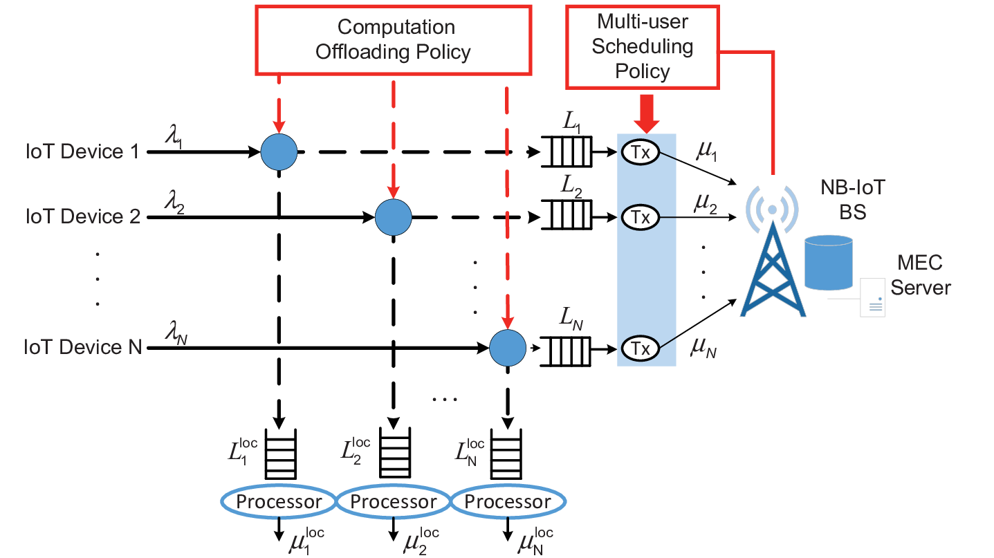
We consider an IoT edge computing system, where a BS with an MEC server serves IoT devices in a singel cell [22]. For each IoT device , the sensed data arrives in packets according to a Poisson distribution of mean arrival rate . There are two queues for each IoT device to buffer the sensed packets. One is the transmission queue for the packets that are to be offloaded to the MEC server for remote computation, and the other is the processing queue for the packets that are be locally processed by the IoT device. When a new packet arrives at an IoT device, the offloading function decides whether to place it in the transmission queue for offloading, or in the processing queue for local processing. Moreover, the multi-user scheduling function in the wireless network decides how to allocate the radio resources to different IoT devices for the transmission of the offloaded packets. The system model for the IoT edge computing system considered in this paper is illustrated in Fig.1.
Assumption 1 (Resource Unit (RU) configuration in NB-IoT)
We consider that the RU configuration with subcarriers time slots is always selected for every IoT device [38]. Therefore, only one IoT device can be scheduled for transmission at the same time.
Assumption 2 (Link adaption in NB-IoT)
In LTE system, link adaptation is performed dynamically per ms subframe to adapt the Modulation and Coding Scheme (MCS) level according to the instantaneous channel quality. As a narrowband transmission technology with a relatively low data rate, the transmission of a transport block (TB) in NB-IoT can occupy multiple consecutive subframes, i.e., a TB may be mapped to RUs in time [38]. This means that the transmission duration can be larger than the coherence time of the wireless channel. Therefore, in this paper, we consider that the link adaptation is performed according to the time-average wireless channel conditions of the IoT devices determined only by the large-scale fading effects, i.e., pathloss and shadowing. Moreover, we focus on those IoT applications where the locations of the IoT devices will not often change once they are deployed, e.g., smart metering. Therefore, the MCS level and the corresponding transmission data rate for an IoT device will remain the same as long as it does not change its location.
As a narrowband transmission technology with a relatively low data rate, the transmission of a transport block in NB-IoT can occupy multiple consecutive subframes [38]. In this paper, we consider that the transmission duration of a packet is exponentially distributed with a mean value , where is the mean transmission rate in terms of packets per second for IoT device . Moreover, the power consumption is a constant value for any IoT device [39].
We consider that the mean local processing time of IoT device is exponentially distributed with a mean of , where is the mean processing rate in terms of packets per second for IoT device . The power consumption for processing the sensed data locally at the IoT device is a constant value denoted by [17].
In this paper, we will try to jointly derive the optimal scheduling policy and computation offloading policy that minimizes the weighted sum of the average delay and power consumption over all the IoT devices. Specifically, the average delay depends on the delay values for both the offloaded as well as the un-offloaded packets. The delay of an offloaded packet includes three parts, i.e., the uplink transmission delay, the remote computation delay, and possibly the downlink transmission delay. We make the following assumption when deriving the average delay for the offloaded packets.
Assumption 3 (Delay for offloaded packets)
We assume that the average delay for the offloaded packets equal to their average uplink transmission delay. This is because the sum of the remote computation delay and the downlink transmission delay is usually neligible compared with the uplink transmission delay and local computation delay due to much more powerful CPUs of the MEC servers and much heavier uplink IoT traffic.
III CTMDP Model
In this section, we shall formulate an infinite horizon average reward Continuous Time Markov Decision Process (CTMDP) problem to minimize the weighted sum of the average delay and power consumption for the IoT devices.
III-A Global System State
We formulate a CTMDP model where the global system states are observed at each packet arrival and departure event. We denote the global system state at the -th decision epoch, , by .
Transmission queue state
is the vector of transmission queue length observed at the beginning of the -th decision epoch when the packet arrival/departure event has just occurred. , denotes the transmission queue length of IoT device , where is the maximum transmission queue length.
Processing queue state
is the vector of processing queue length observed at the beginning of the -th decision epoch, where , denotes the processing queue length of IoT device . is the maximum processing queue length.
Event
Let indicate the event occurred at the beginning of the -th decision epoch which triggers the state transition from to .
-
represents a packet arrival at IoT device ;
-
represents a packet departure from the scheduled transmission queue;
-
represents a packet departure from the processing queue of IoT device , where .
Scheduled transmission queue
is the scheduling action at the last (i.e., -th) decision epoch.
-
represents the index of the scheduled transmission queue at the last (i.e., -th) decision epoch;
-
means no transmission queue is scheduled.
Example 1 (Definition of global system state)
The global system state ( denotes a vector of zeros) indicates that the system state transits to the current state due to a packet arrival at IoT device . At the beginning of the current system state, all the transmission queues and processing queues are empty. No transmission queue is scheduled at the previous system state.
The cardinality of the global system state space is , which grows exponentially with the number of IoT devices .
III-B Action
When a system state transition occurs due to a packet arrival or departure event, an action will be taken in the CTMDP model. Define the action at the -th decision epoch as .
Offloading action
represents the offloading action, which is only performed when there is a packet arrival.
-
means the newly arrived packet is offloaded;
-
means the newly arrived packet is not offloaded; or an offloading action is not applicable in the current system state (i.e., when in the current system state is a packet departure event);
-
means the newly arrived packet is dropped because both the transmission queue and processing queue of the IoT device are saturated.
From the above definition, it is obvious that the offloading action space is dependent on the system state. This dependency is further demonstrated by the fact that if one of two queues (i.e., transmission queue and processing queue) of the IoT device at which the packet arrived is saturated, the packet can only be dispatched to the other queue, and thus the offloading action is determined. Therefore, the state-dependent offloading action space is given as
| (1) |
After the offloading action is made in the -th decision epoch, the arrived packet will be dropped or added to the transmission queue or processing queue of IoT device depending on the offloading action. Therefore, the processing and transmission queue length of IoT device can be different from the values of and in the system state. Let and denote the processing and transmission queue length of any IoT device during the -th decision epoch after the offloading decision is made with system state , we have
| (2) |
and
| (3) |
Define the post-decision transmission and processing queue vectors at the -th decision epoch as and , based on the values of which the scheduling action will be made for the -th decision epoch.
Scheduling action
is the scheduling action.
-
represents the index of the transmission queue that is scheduled at the current (-th) decision epoch;
-
means that no queue is scheduled, which only happens when all the transmission queues are empty at the time the scheduling action is determined, i.e., .;
In this paper, we consider non-preemptive scheduling. Therefore, the scheduling action is only updated when (1) there is a packet departure from a transmission queue (i,e, ); (2) no queue is scheduled at the time that an arrival event occurs (i.e., and ). In either case, the scheduled IoT device is selected from the the set of IoT devices with non-empty transmission queues, i.e., . Otherwise, the scheduling action remains the same as the previous decision epoch (i.e., ). Therefore, the state-dependent scheduling action set is given as
| (4) |
Note that the cardinalities of the offloading action space and scheduling action space are and , respectively.
III-C Post-Decision Global System State
We define the post-decision global system state at the -th decision epoch as , which is a deterministic function of the global system state and the action at the -th decision epoch as below:
| (5) |
Note that the state space of post-decision global system states is the same with that of the global system states as denoted by .
III-D Transition Probability
Given the global systems state and action at the -th decision epoch, the transition to the global systems state at the -th decision epoch can be described in two phases.
- Phase 1
-
where can be derived by (5) as a deterministic function of and ;
- Phase 2
-
where is a deterministic function of and as below:
where , .
Note that the event at the -th decision epoch occurs when there is a packet arrival at any of the IoT devices, or there is a packet departure from the scheduled transmission queue, or from any of the non-empty processing queues. Therefore, the transition probabilities corresponds to the probabilities that event happens:
| (9) |
where we set as will not happen when no transmission queue is scheduled during the -th decision epoch, i.e., .
The duration of the -th decision epoch or equivalently, the sojourn time of the CTMDP in state given action is exponentially distributed with parameter as
| (10) |
where can also be expressed as a function of the post-decision state .
III-E Reward Function
In order to derive the reward function of the CTMDP model, we first examine the optimization objective, which is to find the policy that minimizes the weighted sum of the average delay and power consumption over all the IoT devices. Note that a policy in an MDP model is a function that specifies the action that the decision maker will choose when in state . We formulate the above dynamic optimization problem as an average reward CTMDP problem.
Problem 1 (average reward CTMDP problem to minimize the weighted sum of average delay and power consumption)
| (11) | ||||
where and on the RHS of the first equality are the weights for the average delay and power consumption of IoT device , respectively. The weights and indicate the relative importance of the average delay and power consumption of IoT device in the optimization problem. The RHS of the second equality is the classical form of an average reward CTMDP problem, where and are the starting time and duration of the the -th decision epoch. represents that a reward is incurred at this rate when the system is in state and action is chosen at the the -th decision epoch.
From (11) and using Little’s Law to derive the delay, we can derive the expression of as below:
| (12) |
where is a random variable that takes the value of if the condition in the subscript is true, and otherwise. The detailed derivation is given in Appendix A.
According to the CTMDP theory [40], the reward function of the CTMDP model can be derived as
| (13) |
where can also be expressed as a function of the post-decision state .
The optimal policy of the above CTMDP problem can be derived by solving the post-decision Bellman equation as
| (14) |
where is the post-decision global value function, and is the optimal average reward rate.
IV Solution by DRL
IV-A Local System State
Define the local system state for IoT device at the -th decision epoch as .
- Local event
-
, where
-
indicates a packet arrives at IoT device ;
-
indicates a packet departs from the transmission queue of IoT device ;
-
indicates a packet departs from the processing queue of IoT device ;
-
indicates the event at the -th decision epoch does not happen at IoT device .
- Local schedule
-
, where
-
indicates that IoT device is scheduled at the -th decision epoch;
-
indicates that IoT device is not scheduled at the -th decision epoch.
Given the global system state at the -th decision epoch, the local system state at IoT device can be derived by
| (15) |
| (16) |
The global system state corresponds to the aggregation of the local system states .
Example 2 (Definition of local system state)
Consider there are IoT devices in the system, and the global system state is . Thus, the local system states at the IoT devices are , , and , respectively.
Given the local system state of IoT device at the -th decision epoch, and the action , we define the post-decision local system state , which can be derived by a deterministic function as
| (17) |
Given the post-decision local system state of IoT device at the -th decision epoch, and the event at the -th decision epoch, the local system state of IoT device at the -th decision epoch can be derived by a deterministic function as below by combining (III-D) with the definitions of (post-decision) local system states:
As a remark, note that the cardinality of the local state space for any IoT device is , which does not grow with the number of IoT devices . In contrast, the cardinality of the global state space grows exponentially with the number of IoT devices .
IV-B Value Function Approximation
First, the local reward function is given as
| (22) |
so that .
Moreover, we decompose the optimal average reward rate in (III-E) as the sum of optimal local average reward rates of IoT , i.e.,
| (23) |

In order to formulate our approximation architecture, we first introduce some notations to efficiently describe the mapping relations between the post-decision global system states and the post-decision local system states. Specifically, denote as the -th post-decision global system state in the state space. We introduce a mapping function which denotes the index of the post-decision local system state of device within its local state space when the post-decision global system state is . Therefore, let denote the local system state of device when the global system state is . In other words, we have .
The approximation architecture for the post-decision global value function is given as
| (24) |
where is the cardinality of the local system space of any device , and is the post-decision per-node value function of IoT device for its post-decision local system state . In the following discussion, we’ll omit the term “post-decision” before the global value function and per-node value function for simplicity. is the feature vector of the post-decision global system state . The simplest method is to set for any . However, the feature values of the local system state are the same for all the global system states that belongs to, i.e., the component values within the set are the same. This can lead to inaccuracy in the approximation by (24). In this paper, we will use an ANN to train the values of and simultaneously as shown in Fig.2.
IV-B1 Input layer
The input of the neural network is a post-decision global system state , . The input layer has neurons, where the -th neuron corresponds to the -th post-decision local system state of device , i.e., .
- •
Activation : The activation of the neuron is denoted by , which is a - variable indicating whether is a component of the input post-decision global system state , i.e, . Let be the -dimensional matrix of input neurons where the element in the -th row and -th column is .
IV-B2 Convolutional layer
The number of neurons in the convolutional layer is . The -th neuron corresponds to the device .
- •
Activation : The activation of the -th neuron is denoted by , which represents the convolutional layer feature extracted from the local system state that is encoded by the -th row of . Let be the -dimensional activation vector of the convolutional layer whose -th element is .
- •
C-weight/Filter : The filter is a -dimensional vector , where each element is referred to as the c-weight.
Thus, we have
| (25) |
where denotes the transpose of the matrix .
IV-B3 Fully connected layer
The number of neurons in the fully connected layer is the same with that in the input layer, i.e., , where the -th neuron corresponds to the post-decision local system state .
- •
Activation : The activation of the neuron is denoted by . Let be the -dimensional activation vector of the fully connected layer whose -th element is .
- •
F-weight : The f-weight is the weight of the link from the -th neuron in the convolutional layer to the neuron in the fully connected layer. Let denote the -dimensional matrix of f-weights, whose element in the -th row and the -th column is .
To derive the activation vector of the fully connected layer, we have
| (26) |
where we set to be the Tanh function defined by .
IV-B4 Multiplication layer
Note that when , we would like according to (24). In order to guarantee this, we add a multiplication layer between the fully connected layer and the output layer. There are also neurons in the multiplication layer.
- •
Activation : The activation of the -th neuron is the feature in (24). The -dimensional activation vector whose -th element is can be derived by
(27) where is the Hadamard product or the elementwise product of two vectors.
Remark 1 (Discussion on the multiplication layer)
Note that the neural network and the DRL algorithm still work without the multiplication layer. The advantage of the multiplication layer lies in that it greatly reduces the number of weights or parameters that need to be udpated at each decision epoch. Specifically, among the neurons in the multiplication layer, only neurons are active per decision epoch, which means that only the f-weights and per-node value functions associated with these active neurons need to be updated. This is similar to Dropout in NN, which can prevent overfitting of the value function. Therefore, the multiplication layer not only greatly reduces the computation complexity of the DRL algorithm, but also improves its performance.
IV-B5 Output layer
- •
Activation : The output of the neural network is the global value function of the input post-decision global system state , . Therefore, there is only one output neuron whose activation is .
- •
Weight/Per-node value function : The purpose of the output layer is to derive the global value function of according to (24). The per-node value function is the weight of the link from the neuron in the fully connected layer to the output neuron. Let be the -dimensional per-node value function (weight) vector with the -th element as .
Then, (24) can be written as below
| (28) |
| (24) |
In the following discussion, we will refer to our proposed algorithm as the neural-ICFMO algorithm, which takes the first letter of each neural network layer.
IV-C Optimal Control Action
To illustrate the structure of our solution, we first assume that we could obtain the per-node value function vector , the f-weight matrix , the c-weight vector , and the local optimal average reward rate for every IoT device via somemeans. At the -th decision epoch, we focus on deriving the optimal action under the current system state to minimize the value of the RHS of (24) as below:
| (25) |
Under the system state , the action space is formed by all the actions that is the combination of any eligible offloading action and eligible scheduling action , where and are given by (1) and (4), respectively. The algorithm to determine the optimal control action is given in Algorithm 1.
IV-D Per-Node Value Function and Weight Update
In the above discussion, we consider that all the per-node value functions, f-weights, c-weights, and are known for every IoT device, and derive the optimal control actions based on these values. In this section, we will discuss how to derive the above values using the stochastic gradient (SGD) TD(0) method under function approximation for the average-reward problem [18]. The loss function at the -th decision epoch is defined as
| (26) |
where is the average reward rate of IoT device up to the -th decision epoch. The gradient for the loss function is derived by the well-known backpropagation algorithm for the ANN. The detailed procedures and equations to update the value functions and weights are given in Appendix B and summarized in Algorithm 2 below. Note that at the -th decision epoch, is used in place of in (IV-C) to derive the optimal action . In the following discussion, we add a subscript to the notations described in Section III.B to represent the parameter values at the -th decision epoch.
IV-E Semi-Distributed Implementation of the Solution
The proposed deep reinforcement learning algorithm (i.e., Algorithm 2) can be implemented centrally at the BS. In this case, the BS needs to store the per-node value function vectors, the f-weights and the c-weights for all the IoT devices, whose number grows quadratically instead of exponentially with the number of IoT devices due to the function approximation. Moreover, all the computational tasks for deriving control actions and maintaining the per-node value function vectors, the f-weights and c-weights need to be performed at the BS. On the other hand, the proposed algorithm also allows semi-distributed implementation, in which the BS and IoT devices collaboratively determine the optimal policy as illustrated in Fig.3.
Specifically, we consider that each IoT device stores and updates its own per-node value function vector and the f-weight vectors , . Note that the -dimensional local f-weight vector of IoT device consists of the f-weights from any convolutional neuron , to its local system state . On the other hand, the BS stores and updates the c-weight vector . At the beginning of the -th decision epoch, the BS first derives the convolutional feature vector of the global system state , which corresponds to the activation vector of the convolutional layer of the proposed NN. The BS broadcasts the vector and the value of to the IoT devices, where every IoT device derives a bid for each eligible action under the current system state. The IoT devices submit the bids to the BS, which determine the optimal control action by (IV-C) based on the bid values. The BS notifies the optimal action to the IoT devices, which calculate the values of by (-B) and submit them to the BS. Then, the BS derives the value of by (30) and broadcasts the value to the IoT devices, which updates their per-node value functions and f-weights, respectively. Finally, every IoT device derives the vector by (35) and submits the information to the BS, while the BS updates the c-weights according to (34).

Remark 2 (Signaling overhead of semi-distributed implementation)
The signaling overhead associated with each message in Fig. 3 is listed in Table I. The signaling overhead grows linearly with the number of IoT devices . Note that message ③ is needed irrespective of the implementation method. Messages ④, ⑤, and ⑥ are only needed in the learning phase. After the convergence of the parameters in the neural network, only messages ① and ② are needed. The frequency of the signaling exchange depends on the packet arrival and departure duration of NB-IoT applications, which is typically much longer than the ms time slot in LTE system.
| Message | ① | ② | ③ | ④ | ⑤ | ⑥ |
|---|---|---|---|---|---|---|
| Overhead (bytes) |
V Simulation Results
In this section, we evaluate the performance of our proposed computation offloading and user scheduling algorithm using DRL, i.e., neural-ICFMO, via simulation. Specifically, we compare its performance with the following algorithms:
- •
Queue-aware (QA) algorithm: Both the offloading and scheduling algorithms take into account the queue length and consider load balancing. Specifically, if the transmission queue is shorter than the processing queue at an IoT device, the arrived packet will be offloaded, and vice versa. On the other hand, the IoT device with the largest transmission queue length will be scheduled for transmission.
- •
MUMTO algorithm: We adapt the MUMTO algorithm in [10], which is a typical offloading and resource allocation algorithm designed based on the deterministic task model. Specifically, the optimization objective at the -th decision epoch is , where and are the packet transmission/processing delay and power consumption of IoT device if action is selected at the -th decision epoch.
- •
Neural-ICO algorithm: It is similar to the DQN algorithm used in [23, 25], except that the output from the neural network is the value functions for the post-decision states instead of the Q factors for the state and action pairs. The function approximation architecture of this algorithm is given in Fig.11 in Appendix C.
We developed a discrete-event system-level simulator for the NB-IoT MEC system, where the the simulation parameters are given in Table II. We simulate a circular cell of radius with a BS in the center. The IoT devices are uniformly distributed in the cell area in random. We divide the circular area of the considered cell into disjunct zones by concentric circles around the BS, where the zone is the region between two concentric circles with radius and . We consider that all the IoT devices in zone , select the same MCS level from the MCS levels of the NB-IoT uplink data channel, so that their transmission data rates can be determined according to the Table V in [38]. Then, the mean transmission rate in terms of packets per second for IoT device can be derived as , where is the mean packet size. Note that the MCS level selection schemes are not the focus of this paper, and our proposed offloading and scheduling algorithm can be used for any link adaptation schemes. The transmission power of the IoT device is derived according to the NB-IoT uplink open loop power control formulas given in [39]. The CPU cycles of the IoT devices are considered to be uniformly distributed. Therefore, the mean local processing rate and local power consumption can be derived according to (1) in [8] and (4) in [11], respectively. Without loss of generality, we set the weights of delay and power consumption to be in the reward function. For both the proposed Neural-ICFMO algorithm and the Neural-ICO algorithm, we use the -greedy algorithm to explore the actions. Specifically, the optimal action derived by Algorithm 1 is selected with probability at the -th decision epoch, where with and .
| Parameter | Value |
|---|---|
| Cell radius | m |
| Zone number | |
| Path-loss channel model | |
| m | |
| Maximum transmission power | dBm |
| Number of CPU cycles for processing one bit of data | |
| CPU at the IoT device | cycles/sec |
| The effective switched capacitance of the CPU | |
| Mean packet size | kbits |
| Maximum queue length , | 7 packets |
V-A Performance vs. varying IoT device numbers
We set the packet arrival rate pkts/s. The baseline algorithm QA, the MUMTO algorithm, the proposed Neural-ICFMO algorithm, and the Neural-ICO algorithm are simulated when the number of IoT devices is varied from to . From Fig.4, it can be observed that the proposed Neural-ICFMO algorithm constantly outperforms the other three algorithms in terms of the weighted sum of delay and power consumption, which is the optimization objective as given in (11) for both the Neural-ICFMO and Neural-ICO algorithms. The performance of the QA and the MUMTO algorithms are quite similar, and the performance improvements of the proposed Neural-ICFMO algorithm as well as the Neural-ICO algorithm over these two algorithms increase with the increasing IoT device number. This is because the MUMTO algorithm solves a static optimization problem independently at each decision epoch to optimize the current performance, without considering the impact of the current decision to the long-term time-average performance. Therefore, its performance is not as good as those of the Neural-ICFMO and Neural-ICO algorithms. The proposed Neural-ICFMO algorithm also outperforms the Neural-ICO algorithm due to its neural network architecture for function approximation. Specifically, the neurons in the fully connected layer of the Neural-ICFMO algorithm correspond to the local system states of the IoT devices. This design principle not only facilitates its semi-distributed implementation, but also improves its performance compared with the Neural-ICO algorithm.
Fig.5 and Fig.6 compare the average delay and the power consumption of the four algorithms with increasing IoT device number, respectively. It can be observed that the proposed Neural-ICFMO algorithm achieves the best delay performance, but not the best power consumption performance. This is because the delay value is larger than the power consumption value in our configuration, so that the Neural-ICFMO sacrifices a small amount of power consumption performance to improve a larger amount of delay performance, so that it can achieve the best tradeoff in minimizing the weighted sum of the delay and power consumption. It can also be observed from Fig.6 that the power consumption values can decrease with the increasing IoT device number for the Neural-ICFMO and the Neural-ICO algorithms. For example, the power consumption of Neural-ICFMO is W when and W when . This is because in order to optimize the weighted sum of delay and power consumption, both the Neural-ICFMO and Neural-ICO algorithms may choose to give more priority to minimizing delay or power consumption depending on the specific configuration. Note that the weighted sum of delay and power consumption increases with the increasing IoT device number as given in Fig.4, which makes sense as the increasing IoT device number leads to increasing traffic load and decreasing performance.


V-B Performance vs. varying packet arrival rates
We set the number of IoT devices to be . The four algorithms discussed above are simulated when the packet arrival rate is varied from pkts/s to pkts/s. From Fig.7, it can be observed that the proposed Neural-ICFMO algorithm performs constantly better than the other three algorithms with various packet arrival rates in terms of the weighted sum of delay and power consumption. The baseline QA algorithm outperforms the MUMTO algorithm in this configuration, which demonstrates that load balance is a good strategy. The performance of the Neural-ICO algorithm is approximately the same with that of the proposed Neural-ICFMO algorithm when the arrival rates are small. However, the performance gap between the two algorithms increases with the increasing arrival rate.
Fig.8 and Fig.9 compare the average delay and the power consumption of the four algorithms with increasing arrival rate, respectively. It can be observed that the proposed Neural-ICFMO algorithm achieves the best delay performance and the best power performance under small packet arrival rates. When the packet arrival rate is larger than pkts/s, the MUMTO algorithm achieves the best power performance. However, the delay performance of the MUMTO algorithm is the worst among all the algorithms, and its weighted sum of delay and power consumption is the largest.
V-C Convergence
Fig.10 shows the convergence property of the proposed Neural-ICFMO algorithm and the Neural-ICO algorithm. We plot the value function of global state and the weighted sum of delay and power consumption performance of IoT devices versus the number of decision epochs at a mean arrive rate pkts/s. It can be seen that the value functions of Neural-ICFMO and Neural-ICO algorithms converge at approximately the same speed while their performance improve with increasing number of decision epochs. The performance of Neural-ICFMO is slightly better than that of the Neural-ICO after convergence. The weighted sum of average delay and power consumption for both Neural-ICFMO and Neural-ICO algorithms at the th decision epoch are already smaller than those of the baseline QA and MUMTO algorithms.


VI Conclusion
In this paper, we have proposed a semi-distributed joint computation offloading and multi-user scheduling algorithm based on DRL in NB-IoT edge computing system to minimize the weighted sum of average delay and power consumption over all the IoT devices. Specifically, we consider the stochastic arrival model and formulate the optimization problem into an infinite horizon average reward CTMDP problem. The CTMDP model is based on post-decision states to obtain model-free solution without requiring the knowledge of the underlying stochastic process. In order to deal with the curse-of-dimensionality problem, we use DRL techniques and propose a neural network architecture for approximating the value functions of the post-decision states. The function approximation architecture enables auction-based semi-distributed implementation of the proposed algorithm. Simulation results demonstrate that the proposed algorithm not only outperforms the baseline algorithm, but also RL algorithms based on other function approximation architectures.
-A Derivation of reward rate
According to Little’s Law, the average delay of IoT device can be derived as
| (27) | ||||
where and denote the local processing (no offloading) probability and the offloading probability of IoT device , respectively.
The average power consumption of IoT device can be derived as the sum of the average local processing power consumption and the average transmission power consumption for remote processing,
| (28) |
where represents the probability of IoT device being scheduled so that it will transmit with a power of . On the other hand, represents the probability that the post-decision processing queue states of IoT device is not zero so that it will process the packets with a power of .
-B Procedure for per-node value function and weight updates
Step 1: Per-node value function update
At the -th decision epoch, after the optimal control action is determined, the per-node value function vector is updated based on the observation of the post-decision global and local system states at the -th and -th decision epoch as given below:
| (29) |
where
| (30) |
and
| (31) |
where is a value as close to 1 as possible, e.g., , and enables the algorithm to converge gracefully to the optimal solution. is the number of visits to post-decision local system state for IoT device up to the -th decision epoch, i.e., .
Step 2: F-weight vector update
For every device , update the -dimensional f-weight vector for the links from all the convolutional neurons to the fully connected layer neuron , which corresponds to the transpose of the -th column vector of the matrix .
| (32) |
where
| (33) |
and is the derivative of the Tanh function.
Step 3: C-weight vector update
The c-weight vector is updated as below:
| (34) |
where is an -dimensional vector derived by
| (35) |
Step 4: Average reward update
The average cost rate at IoT device up to the beginning of the -th decision epoch, i.e., , is updated as below:
| (36) |
| (37) |
| (38) |
where is the duration of the -th decision epoch. and are the total accumulative reward and total time up to the beginning of the -th decision epoch, respectively.
Note that and are sequences of step sizes that both satisfy
where represents either or . Moreover, we must make sure that converges to faster than . One example that satisfies this condition is and . Ideally, we have .
-C Function Approximation Architecture for the Neural-ICO algorithm
The function approximation architecture for the Neural-ICO algorithm is given in Fig.11. Note that we have one convolutional layer between the input layer and output layer. We have tried to add a fully connected layer after the convolutional layer, but it turns out that this additional layer does not contribute to improving the performance.

References
- [1] J. Pan and J. McElhannon, “Future edge cloud and edge computing for Internet of Things applications,” IEEE Internet Things J, vol. 5, no. 1, pp. 439-449, Feburary 2018.
- [2] N. Abbas, Y. Zhang, A. Taherkordi, and T. Skeie, “Mobile edge computing: a survey,” IEEE Internet Things J, vol. 5, no. 1, pp. 450-465, Feburary 2018.
- [3] W. Yu, F. Liang, X. He, W.Hatcher, C. Lu, J. Lin, and X. Yang, “A survey on the Edge Computing for the Internet of Things,” IEEE Access, vol. 6, pp. 6900-6919, March 2018.
- [4] G. Premsankar, M. Francesco, and T. Taleb, “Edge computing for the Internet of Things: a case study,” IEEE Internet Things J, vol. 5, no. 2, pp. 1275-1284, April 2018.
- [5] J. Chen, K. Hu, Q. Wang, Y. Sun, Z. Shi, and S. He, “Narrowband Internet of Things: implementations and applications,” IEEE Internet Things J, vol. 4, no. 6, pp. 2309-2314, December 2017.
- [6] J. Xu , J. Yao, L. Wang, Z. Ming, K. Wu, and L. Chen, “Narrowband Internet of Things: evolutions, technologies, and open issues,” IEEE Internet Things J, vol. 5, no. 3, pp. 1449-1462, June 2018.
- [7] H. Malik, H. Pervaiz, M. Alam, Y. Moullec, A. Kuusik, and M. Imran, “Radio resource management scheme in NB-IoT systems,” IEEE Access, vol. 6, pp. 6900-6919, March 2018.
- [8] Y. Mao, C. You, J. Zhang, K. Huang, and K. B. Letaief, “A Survey on Mobile Edge Computing: The Communication Perspective,” IEEE Commun. Surveys Tuts., vol. 19, no. 4, pp. 2322-2358, fourth quarter 2017.
- [9] J. Zhang, W. Xia, F. Yan, and L. Shen, “Joint computation offloading and resource allocation optimization in heterogeneous networks With mobile edge computing,” IEEE Access, vol. 6, pp. 19324-19377, April 2018.
- [10] M. Chen, B. Liang, M. Dong, “Joint offloading decision and resource allocation for multi-user multi-task mobile cloud,” in Proc. IEEE ICC, Kuala Lumpur, Malaysia, May 2016, pp. 1-6.
- [11] Y. Mao, J. Zhang, S. H. Song, and K. B. Letaief, “Stochastic joint radio and computational resource management for multi-user mobile-edge computing systems,” IEEE Trans. Wirel. Commun., vol. 16, no. 9, pp. 5994-6009, September 2017.
- [12] X. Lyu, W. Ni, H. Tian, R. Liu, X. Wang, G. B. Giannakis, and A. Paulraj, “Optimal schedule of mobile edge computing for Internet of Things using partial information,” IEEE J Sel. Area Comm., vol. 35, no. 11, pp. 2606-2615, November 2017.
- [13] Y. Cui and V. K. N. Lau, “Distributive stochastic learning for delay-optimal OFDMA power and subband Allocation”, IEEE Trans. Signal Process., vol. 58, no. 9, pp. 4848-4858, Sept. 2010.
- [14] L. Lei, Y. Kuang, X. Shen, K. Yang, J. Qiao and Z. Zhong, “Optimal Reliability in Energy Harvesting Industrial Wireless Sensor Networks”, IEEE Trans. Wirel. Commun., vol. 15, no. 8, pp. 5399-5413, August 2016.
- [15] J. Liu, Y. Mao, J. Zhang, and K. B. Letaief, “Delay-optimal computation task scheduling for mobile-edge computing systems,” in Proc. IEEE Int. Symp. Inf. Theory (ISIT), Barcelona, Spain, Jul. 2016, pp. 1451-1455.
- [16] S.-T. Hong and H. Kim, “QoE-aware computation offloading scheduling to capture energy-latency tradeoff in mobile clouds,” in Proc. IEEE Int. Conf. Sens. Commun. Netw. (SECON), London, U.K., Jun. 2016, pp. 1-9.
- [17] S. Chen, Y. Wang, and M. Pedram, “A semi-Markovian decision process based control method for offloading tasks from mobile devices to the cloud,” in Proc. IEEE Glob. Commun. Conf. (GLOBECOM), Atlanta, GA, USA, Dec. 2013, pp. 2885-2890.
- [18] R. S. Sutton and A. G. Barto, “Reinforcement Learning: An Introduction”, Second edition in progress, The MIT Press, Cambridge, Massachusetts London, England.
- [19] V. Mnih, et. al., “Human-level control through deep reinforcement learning”, Nature, vol. 518, pp. 529-533, Feb. 2015.
- [20] M. Moghadari, E. Hossain, and L. B. Le, “Delay-optimal distributed scheduling in multi-user multi-relay cellular wireless networks”, IEEE Trans. Commun., vol. 61, no. 4, pp. 1349-1360, April 2013.
- [21] L. Lei, Y. Kuang, N. Cheng, X. Shen, Z. Zhong, and C. Lin, “Delay-optimal dynamic mode selection and resource allocation in Device-to-Device communications—part II: practical algorithm”, IEEE Trans. Veh. Technol., vol. 65, no. 5, pp. 3491-3505, May 2016.
- [22] L. Lei, H. Xu, X. Xiong, K. Zheng, W. Xiang, “Joint computation offloading and multi-user scheduling using approximate dynamic programming in NB-IoT edge computing system”, IEEE Internet Things J, Early Access Article, 2019.
- [23] X. Chen, H. Zhang, C. Wu, S. Mao, Y. Ji, M. Bennis, “Optimized computation offloading performance in virtual edge computing systems via deep reinforcement learning”, IEEE Internet Things J, Early Access Article, 2018.
- [24] Y. Wei, F. R. Yu, M. Song, Z. Han, “Joint Optimization of Caching, Computing, and Radio Resources for Fog-Enabled IoT Using Natural Actor-Critic Deep Reinforcement Learning”, IEEE Internet Things J, Early Access Article, 2018.
- [25] X. He, K. Wang, H. Huang, T. Miyazaki, Y. Wang, S. Guo, “Green resource allocation based on deep reinforcement learning in content-centric IoT”, IEEE Trans. Emerg. Topics Comput., Early Access Article, 2018.
- [26] Z. Chen and X. Wang, “Decentralized computation offloading for multi-user mobile edge computing: A deep reinforcement learning approach,” [Online]. Available: http://arxiv.org/abs/1812.07394.
- [27] L. Huang, X. Feng, C. Zhang, L. Qian, Y. Wu, “Deep reinforcement learning-based joint task offloading and bandwidth allocation for multi-user mobile edge computing,” Digital Communications and Networks, vol. 5, no. 1, pp. 10-17, 2019.
- [28] J. Li, H. Gao, T. Lv and Y. Lu, “Deep reinforcement learning based computation offloading and resource allocation for MEC,” 2018 IEEE Wireless Communications and Networking Conference (WCNC), Barcelona, 2018, pp. 1-6.
- [29] Y. Wei, Z. Zhang, F. R. Yu and Z. Han, “Joint User Scheduling and Content Caching Strategy for Mobile Edge Networks Using Deep Reinforcement Learning”, in 2018 IEEE International Conference on Communications Workshops (ICC Workshops), Kansas City, MO, 2018, pp. 1-6.
- [30] J. Wang, L. Zhao, J. Liu, and N. Kato, “Smart resource allocation for mobile edge computing: A deep reinforcement learning approach,” IEEE Transactions on Emerging Topics in Computing, Early Access Article, March 2019.
- [31] M. L. Littman, “Markov games as a framework for multi-agent reinforcement learning”, in Proceedings of the eleventh international conference on machine learning, vol. 157, pp. 157–163, 1994.
- [32] M. Tan, “Multi-agent reinforcement learning: Independent vs. cooperative agents”, in Proceedings of the tenth international conference on machine learning, pp. 330–337, 1993.
- [33] J. Foerster, “Stabilising Experience Replay for Deep Multi-Agent Reinforcement Learning”, https://arxiv.org/abs/1702.08887, 2018.
- [34] T. T. Nguyen, N. D. Nguyen, and S. Nahavandi, “Deep reinforcement learning for multi-agent systems: A review of challenges, solutions and applications”, arXiv preprint arXiv:1812.11794, 2018.
- [35] L. Busoniu, R. Babuska, and B. De Schutter, “A comprehensive survey of multi-agent reinforcement learning,” IEEE Transactions on Systems, Man, and Cybernetics, Part C: Applications and Reviews, vol. 38, no. 2, pp. 156–172, Mar. 2008.
- [36] P. Hernandez-Leal, M. Kaisers, T. Baarslag, E. M. de Cote, “A Survey of Learning in Multiagent Environments: Dealing with Non-Stationarity”, https://arxiv.org/abs/1707.09183, 2019.
- [37] L. Lei, Z. Zhong, C. Lin, and S. Shen, “Operator controlled device-to-device communications in LTE-advanced networks,” IEEE Wireless Mag., vol. 19, no. 3, pp. 96-104, June 2012.
- [38] R. Ratasuk, N. Mangalvedhe, J. Kaikkonen and M. Robert, “Data Channel Design and Performance for LTE Narrowband IoT,” in Proc. 2016 IEEE VTC-Fall, Sept. 2016, pp.1-5.
- [39] C. Yu, L. Yu, Y. Wu, Y. He, and Q. Lu, “Uplink scheduling and link adaptation for Narrowband Internet of Things systems”, IEEE Access, vol.5, pp.1724-1734, Feb. 2017.
- [40] M. L. Puterman, Markov Decision Processes: Discrete Stochastic Dynamic Programming, New York: Wiley, 1994.