Characterizing the Uncertainty of Jointly Distributed Poses in the Lie Algebra

The Special Euclidean group, or $\mathrm{SE}(d)$, represents the space of homogeneous transformation matrices or the space of matrices that apply a rigid body rotation and translation to points in $\mathbb{R}^{d}$ (represented in homogeneous form). Formally, in three dimensions, $\mathrm{SE}(3)$ is defined as follows:

where $\mathrm{SO}(3)$ is the Special Orthogonal group is the space of valid rotation matrices:

and $\mathbf{I}_{d}$ is the identity matrix of dimension $d$. A variety of methods have been developed for parameterizing these objects such as Euler angles or quaternions [6].

Both $\mathrm{SE}(3)$ and $\mathrm{SO}(3)$ are matrix Lie groups meaning they are smooth manifolds that also satisfy the formal definition of a mathematical group [12, 13] with the standard matrix multiplication operation. Intuitively, this means that while the general group is non-linearm, each of these groups can be locally approximated using a Euclidean vector space. Additionally, for any given point on the manifold, consider the set of all paths on the manifold that pass through that point. The set of all velocities (both in terms of direction and speed) of those paths at the given point form a vector space called the tangent space. The tangent space centered at the identity is called the Lie algebra. This relationship is depicted in Fig. 2.

The Lie algebra of $\mathrm{SO}(3)$ is denoted $\mathfrak{so}(3)$ and is the space of skew-symmetric $3\times 3$ matrices [14, 12]:

This space is isomorphic to $\mathbb{R}^{3}$ since skew-symmetric matrices have zeros on the diagonal entries and the lower entries are completely identified by three upper entries (hence $\mathrm{dim}~\mathfrak{so}(3)=3$). Therefore, it is very convenient to work with $\mathbb{R}^{3}$ instead. Note, we can use the $\wedge$ operator to take an element of $\mathbb{R}^{3}$ and transform it to an element of $\mathfrak{so}(3)$:

where $\boldsymbol{\phi}\in\mathbb{R}^{3}$. The $\vee$ operator denotes the inverse of $\wedge$.

Similarly, the Lie algebra of $\mathrm{SE}(3)$, or $\mathfrak{se}(3)$, is defined as follows:

This space of matrices is isomorphic to $\mathbb{R}^{6}$ and we overload the $\wedge$ operator to convert between the Euclidean vector and matrix forms:

where $\boldsymbol{\xi}\in\mathbb{R}^{6}$ and $\boldsymbol{\rho},\boldsymbol{\phi}\in\mathbb{R}^{3}$.

Understanding the relationship between the group and algebra spaces can enable one to leverage the fact that the algebra is a vector space. The next few subsections cover some important concepts from Lie group Theory that we need in the rest of the paper. In doing so, we use $\mathcal{G}$ to represent a given Lie group and $\mathfrak{g}$ to represent its associated Lie algebra.

The Lie algebra, $\mathfrak{g}$, represents the tangent space of the manifold at the identity. However, given a specific tangent vector, we may want to convert it to its associated transformation in the group space $\mathcal{G}$. The exponential map, $\operatorname{exp}:\mathfrak{g}\rightarrow\mathcal{G}$, (which can be defined in closed form for $\mathrm{SE}(3)$), enables us to perform this conversion,

The logarithm map, $\operatorname{log}:\mathcal{G}\rightarrow\mathfrak{g}$, on the other hand, enables us to go the other direction from an action/transformation in the group space to the velocity that would have induced it,

This relationship is visualized in Fig. 2.

Assuming $\mathbf{T}\in\mathcal{G}$ and $\boldsymbol{\xi}\in\mathfrak{g}$, the adjoint action of $\mathbf{T}$ on $\boldsymbol{\xi}$, or $\operatorname{Ad}_{\mathbf{T}}(\boldsymbol{\xi})$ is defined as follows:

The adjoint action describes the affect that transforming to the group space applying a transformation on the left and its inverse on the right has on an element of the Lie algebra. This gives rise to the following property, which we use later on:

Finally, we also want to characterize the effect that multiplication in the group space has on the Lie algebra. More specifically, suppose we want to compute the Lie algebra element, $\boldsymbol{\xi}_{ac}\in\mathfrak{g}$, that is generated by taking the logarithm of the product of the exponential of two Lie algebra elements $\boldsymbol{\xi}_{ab},\boldsymbol{\xi}_{bc}\in\mathfrak{g}$. The Baker-Campbell-Hausdorff (BCH) formula describes this relationship purely in the Lie algebra space without requiring the application of the exponential or the logarithm:

where $[\cdot,\cdot]$ is the Lie bracket of $\mathfrak{g}$ [15, (7.18)]. For brevity, in the special case where we consider elements in $\mathrm{SE}(3)$, we adopt the notation of [1]:

which allows us to write the BCH formula as:

Finally, as discussed in [1], one can define random variables for $\mathrm{SE}(3)$ according to

where $\bar{\mathbf{T}}_{\ell}\in\mathrm{SE}(3)$ is a ‘large’ noise free value and $\boldsymbol{\xi}_{\ell}\in\mathbb{R}^{6}$ is a ‘small’ noisy perturbation (using the nomenclature of [1]). Two examples of this noisy perturbation are depicted in the middle row of Fig. 1. By defining $\boldsymbol{\xi}_{\ell}$ to be a zero-mean Gaussian random variable $\boldsymbol{\xi}_{\ell}\sim\mathcal{N}(\mathbf{0},\mathbf{\Sigma}_{\ell})$ in the Lie algebra, we induce a probability distribution function over $\mathrm{SE}(3)$ that is parameterized with a mean $\bar{\mathbf{T}}_{\ell}\in\mathrm{SE}(3)$ and a covariance $\mathbf{\Sigma}_{\ell}$ defined in the Lie algebra [1].

We use these properties in Sections IV, V, VI, and VII to propose a framework for modeling jointly correlated poses and to derive uncertainty propagation formulas for the operations in Fig. 3. However, we first review the SSC coordinate based method.

Under SSC notation, the relative transformation between the coordinate frame $i$ and $j$, or the pose of coordinate frame $j$ with respect to frame $i$, is denoted by

where $x_{ij}$, $y_{ij}$, and $z_{ij}$ are position coordinates and $\phi_{ij}$, $\theta_{ij}$, and $\psi_{ij}$ are Euler angles that encode the position and orientation of the coordinate frame $j$ with respect to the frame $i$. However, because each relative transformation is derived from noisy measurements, our estimate is uncertain and we do not know the true value of $\mathbf{x}_{ij}$. Instead, we track a nominal mean value of its parameters and an associated $6\times 6$ covariance matrix, $\hat{\mathbf{x}}_{ij}$ and $\mathbf{\Sigma}_{\mathbf{x}_{ij}}$, respectively.

The stochastic map, proposed in [5], treats all of the uncertain transformations as jointly Gaussian multivariate random variables by stacking them into a single state vector $\mathbf{x}$ and tracking the mean and covariance of that state. Assuming we have $n$ relative transformations we want to track, if we index them from $a=1,\dots,n$, then $\mathbf{x}$ and its associated mean and covariance are:

where $\mathbf{x}$ is a vector of length $6n$, $\mathbf{\Sigma}_{\mathbf{x}_{a}}$ is the $6\times 6$ covariance matrix of the relative transformation $\mathbf{x}_{a}$ and the off diagonal blocks of the form $\mathbf{\Sigma}_{\mathbf{x}_{a}\mathbf{x}_{b}}$ are the respective $6\times 6$ cross covariance matrices.

Suppose we are given a noisy observation of a robot’s relative pose between time steps $i$ and $j$ $(\mathbf{x}_{ij})$ and another observation of its relative pose between time steps $j$ and $k$ $(\mathbf{x}_{jk})$, we may want to calculate the relative pose between time steps $i$ and $k$ $(\mathbf{x}_{ik})$ by composing the observations $\mathbf{x}_{ij}$ and $\mathbf{x}_{jk}$ (see Fig. 3). The SSC head-to-tail operation is a nonlinear function $f_{\oplus}:\mathbb{R}^{6}\times\mathbb{R}^{6}\rightarrow\mathbb{R}^{6}$ that takes the parameter vectors $\mathbf{x}_{ij}$ and $\mathbf{x}_{jk}$ as input and outputs the parameter vector $\mathbf{x}_{ik}$ that results from composing the respective homogeneous transformation matrices. The $\oplus$ operator denotes this operation:

The mean and covariance of the resulting pose are estimated up-to first order as

and

where $J_{\oplus}(\hat{\mathbf{x}}_{ij},\hat{\mathbf{x}}_{jk})$ is the Jacobian of $f_{\oplus}$ at $\hat{\mathbf{x}}_{ij}$ and $\hat{\mathbf{x}}_{jk}$, and

Suppose we are given a robotic vehicle that is tasked with navigating through an a priori unknown environment after which it must return to the origin location. While it is common to represent the robotic vehicle’s current location with respect to the origin using estimation theory, it may be useful to instead characterize the pose of the origin with respect to the local robot coordinate frame. Formally, given an uncertain estimate of the pose of coordinate frame $j$ with respect to frame $i$ ($\mathbf{x}_{ij}$), we want to determine the pose of frame $i$ with respect to frame $j$ ($\mathbf{x}_{ji}$). This amounts to finding the vector $\hat{\mathbf{x}}_{ji}$ that corresponds to the inverse of $\hat{\mathbf{x}}_{ij}$ (in terms of homogeneous transformation matrices) and representing the uncertainty with respect to this new frame of reference.

The SSC pose inverse operation is a nonlinear function $f_{\ominus}:\mathbb{R}^{6}\rightarrow\mathbb{R}^{6}$ takes a pose and computes the inverse of the pose as a homogeneous transformation matrix:

The mean and covariance of the resulting pose are estimated up-to first order as

and

where $J_{\ominus}(\hat{\mathbf{x}}_{ij})$ is the Jacobian of $f_{\ominus}$ at $\hat{\mathbf{x}}_{ij}$.

Finally, the SSC tail-to-tail operation takes uncertain estimates of two coordinate frames with respect to a single origin frame and evaluates the relative pose between them. More succinctly, given $\mathbf{x}_{ij}$ and $\mathbf{x}_{ik}$, find $\mathbf{x}_{jk}$. This operation is useful when using a method such as pose graph SLAM (SLAM) for navigation since the robot pose at multiple time steps is often estimated with respect to a single fixed coordinate frame.

The SSC relative pose operation is a nonlinear function $f_{\ominus\oplus}:\mathbb{R}^{6}\times\mathbb{R}^{6}\rightarrow\mathbb{R}^{6}$ that is defined by first applying the inverse and then the head-to-tail operation:

The mean and covariance of the resulting pose up-to first order are estimated as

and

where $J_{\ominus\oplus}(\hat{\mathbf{x}}_{ij},\hat{\mathbf{x}}_{ik})$ is the Jacobian of $f_{\ominus\oplus}$ at $\hat{\mathbf{x}}_{ij}$ and $\hat{\mathbf{x}}_{ik}$, and

Suppose we have two uncertain poses $\mathbf{T}_{ij}$ and $\mathbf{T}_{jk}$ with perturbations $\boldsymbol{\xi}_{ij}$ and $\boldsymbol{\xi}_{jk}$ that are jointly Gaussian in the Lie algebra with covariance matrix

Our goal is to find the mean and covariance of $\mathbf{T}_{ik}$, $\{\bar{\mathbf{T}}_{ik},\mathbf{\Sigma}_{ik}\}$. Under the standard group multiplication operation:

Following the random variable definition in (14) and using the property described in (10),

where $\mathrm{Ad}_{\bar{\mathbf{T}}_{ij}}$ is the matrix form of the adjoint action of $\bar{\mathbf{T}}_{ij}$ on $\mathfrak{se}(3)$. Letting

gives us

We can now use the BCH (BCH) formula (13) to show that

where $\boldsymbol{\xi}^{\prime}_{jk}=\mathrm{Ad}_{\bar{\mathbf{T}}_{ij}}\boldsymbol{\xi}_{jk}$. Computing the covariance $\mathbf{\Sigma}$ amounts to evaluating $E[\boldsymbol{\xi}_{ik}\boldsymbol{\xi}_{ik}^{\top}]$. Multiplying out up-to fourth order, we get:

This derivation is identical to the one proposed in [1] until the last step. Since [1] assumes the individual poses are independent, the cross terms in (47) and (49) are zero and the evaluation of the 4th order terms in (48) is simplified. If this assumption is true and $\boldsymbol{\xi}_{ij}$ and $\boldsymbol{\xi}^{\prime}_{jk}$ are independent of one another, as is the case when $\mathbf{T}_{ij}$ and $\mathbf{T}_{jk}$ are independent measurements of consecutive robot motion, then the cross terms in (48) and the covariance $\mathbf{\Sigma}$ can be calculated up to 4th order as described in [1]. However, if the poses $\mathbf{T}_{ij}$ and $\mathbf{T}_{jk}$ are correlated, as is often the case when they are derived from the solution of a MLE (MLE) problem such as Pose Graph SLAM or in the case of wheel slip, the cross terms must be included and evaluation of the fourth order terms in (48) and (49) becomes more difficult¹¹ 1 If increased accuracy is needed then Isserlis Theorem can be applied to evaluate the fourth order terms in (48) and (49).. If the correlation is not taken into account, then the result of the pose composition operation under-approximates the true distribution and consistency is lost as shown in Fig. 4.

A first order estimate of covariance (second order in the perturbation variables) can be obtained be evaluating

resulting in

Thus, first order pose composition on the Lie algebra can be performed for correlated poses using (44) for mean propagation and (51) for covariance propagation. As noted previously, this is equivalent to the first order method presented in [1] with the exception of the two additional cross terms in (51) needed to model cross correlation.

While both the SSC operations presented in [5] and the Lie algebra based methods presented in this paper (and $\Sigma_{2nd}$ in [1, (55)]) are first order approximation methods (in terms of covariance), characterizing rotation uncertainty in the Lie algebra space results in a more accurate characterization of pose uncertainty. This is because Euler angle parameterization is a chart and does not cover the entire manifold whereas the Lie algebra inherently captures the group structure and can model any arbitrary group element. In addition, since the Lie algebra is a vector space [12], modeling the uncertainty as a Gaussian distribution is convenient and well-defined.

To demonstrate this, we performed an experiment similar to the one proposed in [1]. We generated a sequence of $N$ noisy pose transformations of the form $\mathbf{T}_{ab}=\operatorname{exp}(\boldsymbol{\xi}_{ab}^{\wedge})\bar{\mathbf{T}}_{ab}$, with

and

where $\sigma_{t}$ and $\sigma_{r}$ are scaling parameters for the translation and rotation noise respectively. In addition, each consecutive perturbation variable $\boldsymbol{\xi}_{ab}$ was drawn such that it was correlated with the perturbation variable before it with correlation coefficient $\rho$.

We then composed these transformations end-to-end and repeated the process to generate 10000 sample trajectories. These Monte-Carlo simulation results were then used to evaluate the uncertainty predicted by the SSC head-to-tail operation as well as the Lie-algebra based pose composition method derived in this section, both with and without correlation being taken into account. A top down view of one such experiment with $N=10$, $\sigma_{t}=5$, $\sigma_{r}=5$, and $\rho=0.4$ is shown in Fig. 4.

As expected, the Lie algebra based method significantly outperforms SSC head-to-tail because it takes into account the structure of the $\mathrm{SE}(3)$ group. In addition, it is easily seen that dropping the cross covariance terms results in an under-approximation of the true covariance, if positive correlation is indeed present. A more thorough investigation of this experiment is described in §IX-A.

In the next two sections, we provide a derivation of the inverse and relative pose operations on the Lie algebra, which as far as we know have not been previously published.

Given uncertain estimates of two coordinate frames with respect to a common base frame, our aim is estimate the relative transformation between the two poses. For example, given possibly correlated uncertain transformations $\mathbf{T}_{ij}$ and $\mathbf{T}_{ik}$ representing the poses of coordinate frames $j$ and $k$ with respect to frame $i$, we want to find the mean $\bar{\mathbf{T}}_{jk}$ and covariance $\mathbf{\Sigma}_{jk}$ that parameterize the pose uncertainty of frame $k$ with respect to frame $j$.

We start by assuming that the $\bar{\mathbf{T}}_{ij}$ and $\bar{\mathbf{T}}_{ik}$ are known and that the associated perturbations $\boldsymbol{\xi}_{ij}$ and $\boldsymbol{\xi}_{ik}$ are jointly correlated in the Lie algebra with known covariance

Under the standard group inverse and multiplication actions, the following must hold:

Expanding (60) using the random variable definition in (14) and the derivation in (55) results in

where $\boldsymbol{\xi}_{ij}^{\prime}=-\mathrm{Ad}_{\bar{\mathbf{T}}_{ij}^{-1}}\boldsymbol{\xi}_{ij}$ and $\boldsymbol{\xi}_{ik}^{\prime}=\mathrm{Ad}_{\bar{\mathbf{T}}_{ij}^{-1}}\boldsymbol{\xi}_{ik}$. Letting

gives us

Expanding the BCH formula in a similar manner to (46) and taking the expectation as in (47) results in the following up to first order:

Evaluating the expectations in (64) results in

Thus, uncertainty can be propagated through the relative pose function via (62) and (65). A summary of the uncertainty propagation methods derived in the last three sections is provided in Fig. 3.

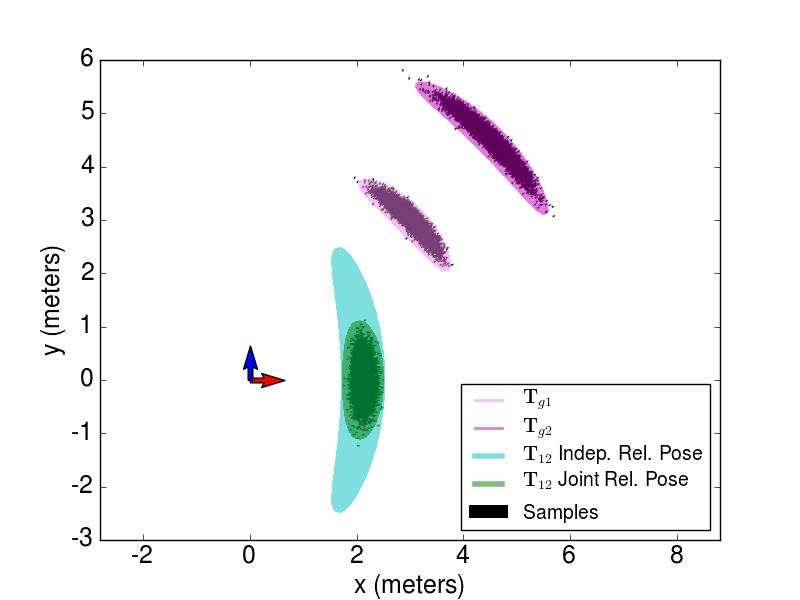
Ignoring correlation of the associated perturbation variables leads to under/over-estimation of uncertainty, depending on if the correlation is positive or negative and if the operation being performed is pose composition or relative pose estimation. Fig. 5 and Fig. 6 show an example of this for the case of relative pose with positive correlation.

To create these plots, we generated $M=10000$ sets of two uncertain poses $\mathbf{T}^{m}_{g1}=\operatorname{exp}(\boldsymbol{\xi}_{g1}^{m\wedge})\bar{\mathbf{T}}_{g1}$ and $\mathbf{T}_{g2}=\operatorname{exp}(\boldsymbol{\xi}_{g2}^{m\wedge})\bar{\mathbf{T}}_{g2}$, with mean values

and

under the assumption that the perturbation variables ($\boldsymbol{\xi}^{m}_{g1}$) and ($\boldsymbol{\xi}^{m}_{g2}$) are jointly correlated in the Lie algebra with marginal covariance matrices

and cross covariance

where $\alpha$ is a scaling parameter. We then used the relative pose operation presented in this section to estimate $\mathbf{T}_{12}$ both with and without taking uncertainty into account.

In Fig. 6, we evaluate the estimated covariance error for increasing values of $\alpha$ with respect to the Monte-Carlo simulation under the following covaraiance error metric

where

with

and

Fig. 4, Fig. 5, and Fig. 6 show that ignoring correlation leads to inconsistent estimates of uncertainty.

Assuming we are given a mean parameter vector $\hat{\mathbf{x}}$ and associated covariance $\hat{\boldsymbol{\Sigma}}$ as defined in (III-A), to apply our proposed propagation methods, we must first transform $\hat{\mathbf{x}}$ and $\hat{\boldsymbol{\Sigma}}$ into into our proposed representation such that the means of the associated transformations are represented in the group space via $\bar{\mathbf{T}}_{1:n}$ and the perturbations are represented as multivariate Guassian random variables, $\boldsymbol{\xi}_{1:n}$, with covariance $\boldsymbol{\Sigma}_{1:n}$ in the associated Lie algebra as defined in (38) and (39). Converting from a coordinates based method for uncertainty characterization to the Lie algebra representation is a non-linear operation. As such, the unscented transform [23] is a better choice for converting between representations than a first order linearization method.

The unscented transform, first proposed by Julier and Uhlmann 1997 in 1997, takes an input Gaussian distribution defined in one space and a non-linear function that maps the input space to an output space and finds a Gaussian approximation for the transformed distribution. This is done by using the input mean and covariance to create a deterministic set $\mathcal{X}_{1:K}$ of $K=2m+1$ sigma points, where $m$ is the dimension of the input space. These sigma points are then passed through the non-linear function and a weighted mean and sample covariance is used to find a Gaussian approximation to the output distribution.

Assuming we have a function $f:\mathbb{R}^{d}\mapsto\mathcal{G}$ that maps from a parameter vector, $\mathbf{x}_{i}$, to an element of the Lie group, $\mathcal{G}$, we can define a function $\ell_{i}$ that takes a perturbed parameter vector $\tilde{\mathbf{x}}_{i}$, centers it on the identity, and transforms it to the Lie algebra space as follows:

where $\hat{\mathbf{x}}_{i}$ is the mean parameter vector associated with $\tilde{\mathbf{x}}_{i}$.

We can then use the standard unscented transform [24, (12)] to generate a set $\mathcal{X}_{1:K}$ of $2nd+1$ sigma points from $\hat{\mathbf{x}}$ and $\hat{\boldsymbol{\Sigma}}$, where $n$ is the number of modeled Lie group elements. After which, the predicted Lie group representation for the jointly correlated poses can be obtained as follows:

where $\ell$ is a vectorized version of $\ell_{i}$ and $\mathcal{W}_{k}$ is the standard weight from [24, (12)]. Fig. 7 shows a result of this process.

References

- Barfoot and Furgale [2014] T. D. Barfoot and P. T. Furgale, “Associating uncertainty with three-dimensional poses for use in estimation problems,” IEEE Trans. on Robotics, vol. 30, no. 3, pp. 679–693, 2014.
- Dissanayake et al. [2001] M. G. Dissanayake, P. Newman, S. Clark, H. F. Durrant-Whyte, and M. Csorba, “A solution to the simultaneous localization and map building (SLAM) problem,” IEEE Trans. Robot. Autom., vol. 17, no. 3, pp. 229–241, 2001.
- Thrun et al. [2005] S. Thrun, W. Burgard, and D. Fox, Probabilistic robotics. MIT press, 2005.
- Smith and Cheeseman [1986] R. C. Smith and P. Cheeseman, “On the representation and estimation of spatial uncertainty,” Int. J. Robot. Res., vol. 5, no. 4, pp. 56–68, 1986.
- Smith et al. [1990] R. Smith, M. Self, and P. Cheeseman, “Estimating uncertain spatial relationships in robotics,” Auton. Robot., pp. 167–193, 1990.
- Spong et al. [2005] M. W. Spong, S. Hutchinson, and M. Vidyasagar, Robot modeling and control. Wiley New York, 2005.
- Murray et al. [1994] R. M. Murray, Z. Li, and S. Shankar Sastry, A mathematical introduction to robotic manipulation. CRC press, 1994.
- Huang and Dissanayake [2007] S. Huang and G. Dissanayake, “Convergence and consistency analysis for extended kalman filter based SLAM,” IEEE Trans. on Robotics, vol. 23, no. 5, pp. 1036–1049, 2007.
- Rodríguez-Arévalo et al. [2018] M. L. Rodríguez-Arévalo, J. Neira, and J. A. Castellanos, “On the importance of uncertainty representation in active slam,” IEEE Trans. on Robotics, 2018.
- Wang and Chirikjian [2008] Y. Wang and G. S. Chirikjian, “Nonparametric second-order theory of error propagation on motion groups,” The International journal of robotics research, vol. 27, no. 11-12, pp. 1258–1273, 2008.
- Long et al. [2012] A. W. Long, K. C. Wolfe, M. J. Mashner, and G. S. Chirikjian, “The banana distribution is gaussian: A localization study with exponential coordinates,” Proc. Robot.: Sci. & Syst. Conf., vol. 265, Jul 2012.
- Tapp [2016] K. Tapp, Matrix groups for undergraduates. American Mathematical Soc., 2016, vol. 79.
- Baker [2012] A. Baker, Matrix groups: An introduction to Lie group theory. Springer Science & Business Media, 2012.
- Chirikjian [2011] G. S. Chirikjian, Stochastic Models, Information Theory, and Lie Groups, Volume 2: Analytic Methods and Modern Applications. Springer Science & Business Media, 2011.
- Barfoot [2017] T. D. Barfoot, State Estimation for Robotics. Cambridge University Press, 2017.
- Kim and Kim [2017] Y. Kim and A. Kim, “On the uncertainty propagation: Why uncertainty on lie groups preserves monotonicity?” in Proc. IEEE/RSJ Int. Conf. Intell. Robots and Syst., Vancouver, BC, Canada, Sep. 2017, pp. 3425–3432.
- Forster et al. [2017] C. Forster, L. Carlone, F. Dellaert, and D. Scaramuzza, “On-manifold preintegration for real-time visual–inertial odometry,” IEEE Transactions on Robotics, vol. 33, no. 1, pp. 1–21, 2017.
- Hartley et al. [2018] R. Hartley, J. G. Mangelson, L. Gan, M. G. Jadidi, J. M. Walls, R. M. Eustice, and J. W. Grizzle, “Legged robot state-estimation through combined forward kinematic and preintegrated contact factors,” in Proc. IEEE Int. Conf. Robot. and Automation, Brisbane, Australia, May 2018, pp. 1–8.
- Wheeler et al. [2018] D. O. Wheeler, D. P. Koch, J. S. Jackson, T. W. McLain, and R. W. Beard, “Relative navigation: A keyframe-based approach for observable gps-degraded navigation,” IEEE Control Syst. Mag., vol. 38, no. 4, pp. 30–48, 2018.
- [20] E. Eade, “Lie groups for 2D and 3D transformations,” accessed: 2018-12-05. [Online]. Available: http://ethaneade.com/lie.pdf
- Kaess et al. [2008] M. Kaess, A. Ranganathan, and F. Dellaert, “iSAM: Incremental smoothing and mapping,” IEEE Trans. on Robotics, vol. 24, no. 6, pp. 1365–1378, 2008.
- Kümmerle et al. [2011] R. Kümmerle, G. Grisetti, H. Strasdat, K. Konolige, and W. Burgard, “g2o: A general framework for graph optimization,” in Proc. IEEE Int. Conf. Robot. and Automation, Shanghai, China, May 2011, pp. 3607–3613.
- Julier [2002] S. J. Julier, “The scaled unscented transformation,” in Proc. Amer. Control Conf., vol. 6, Anchorage, Alaska, USA, May 2002, pp. 4555–4559.
- Julier and Uhlmann [1997] S. J. Julier and J. K. Uhlmann, “New extension of the kalman filter to nonlinear systems,” in Signal processing, sensor fusion, and target recognition VI, vol. 3068. International Society for Optics and Photonics, 1997, pp. 182–194.
- Dellaert and Kaess [2006] F. Dellaert and M. Kaess, “Square Root SAM: Simultaneous localization and mapping via square root information smoothing,” Int. J. Robot. Res., vol. 25, no. 12, pp. 1181–1203, 2006.
- Kaess et al. [2012] M. Kaess, H. Johannsson, R. Roberts, V. Ila, J. J. Leonard, and F. Dellaert, “iSAM2: Incremental smoothing and mapping using the bayes tree,” Int. J. Robot. Res., vol. 31, no. 2, pp. 216–235, 2012.
- Rosen et al. [2016] D. Rosen, L. Carlone, A. Bandeira, and J. Leonard, “SE-Sync: A certifiably correct algorithm for synchronization over the Special Euclidean group,” in Proc. Int. Work. Algorithmic Foundations of Robot., 2016.
- Mangelson et al. [2019] J. G. Mangelson, J. Liu, R. M. Eustice, and R. Vasudevan, “Guaranteed globally optimal planar pose graph and landmark slam via sparse-bounded sum-of-squares programming,” in Proc. IEEE Int. Conf. Robot. and Automation, Montreal, Canada, May 2019, pp. 1–8.
- Kaess and Dellaert [2009] M. Kaess and F. Dellaert, “Covariance recovery from a square root information matrix for data association,” Journal of Robotics and Autonomous Systems, RAS, vol. 57, no. 12, pp. 1198–1210, December 2009.
- Olson et al. [2006] E. Olson, J. Leonard, and S. Teller, “Fast iterative alignment of pose graphs with poor initial estimates,” in Proc. IEEE Int. Conf. Robot. and Automation, Orlando, Florida, May 2006, pp. 2262–2269.
- Mangelson et al. [2018] J. G. Mangelson, D. Dominic, R. M. Eustice, and R. Vasudevan, “Pairwise consistent measurement set maximization for robust multi-robot map merging,” in Proc. IEEE Int. Conf. Robot. and Automation, Brisbane, Australia, May 2018, pp. 1–8.
![[Uncaptioned image]](1906.07795v1/figures/jman_small.jpg) |
Joshua Mangelson received the B.S. degree in electrical engineering from Brigham Young University, Provo, UT, USA in 2014 and the M.S. degree in robotics from the University of Michigan, Ann Arbor, MI, USA in 2016. He is currently a Ph.D. candidate in robotics at the University of Michigan with expected completion in April 2019. His research interests lie in the development of navigation, mapping, perception, and planning algorithms with mathematical and performance guarantees that enable the design of reliable field robotic systems for operation in unstructured environments. He is especially interested in the development of large-scale multi-agent teams for autonomous inspection of underwater structures. He is the recipient of the IEEE ICRA Best Multi-Robot Paper Award and the IEEE OCEANS Best Poster Award both in 2018. |
![[Uncaptioned image]](1906.07795v1/figures/mgj.jpg) |
Maani Ghaffari received the Ph.D. degree from the Centre for Autonomous Systems (CAS), University of Technology Sydney, NSW, Australia, in 2017. He is currently an Assistant Research Scientist at the Robotics Institute and Department of Naval Architecture and Marine Engineering, University of Michigan, Ann Arbor, MI, USA. His research interests include applied mathematics, robotic perception, machine learning, and planning under uncertainty with applications in robotics and autonomous systems. |
![[Uncaptioned image]](1906.07795v1/figures/RamVasudevan.JPG) |
Ram Vasudevan received the B.S. degree in electrical engineering and computer sciences, the M.S. degree in electrical engineering, and the Ph.D. degree in electrical engineering from the University of California at Berkeley in 2006, 2009, and 2012, respectively. He is currently an Assistant Professor in mechanical engineering with the University of Michigan, Ann Arbor, with an appointment in the University of Michigan’s Robotics Program. His research interests include the development and application of optimization and systems theory to quantify and improve human and robot interaction. |
![[Uncaptioned image]](1906.07795v1/figures/RME.jpg) |
Ryan M. Eustice received the B.S. degree in mechanical engineering from Michigan State University, East Lansing, MI, USA, in 1998 and the Ph.D. degree in ocean engineering from the Joint Program between the Massachusetts Institute of Technology (MIT), Cambridge, MA, USA and the Woods Hole Oceanographic Institution (WHOI), Woods Hole, MA, USA, in 2005. Currently, he is the Senior Vice President of Automated Driving at the Toyota Research Institute and a Professor with the Department of Naval Architecture and Marine Engineering, University of Michigan, Ann Arbor, MI, USA, with joint appointments in the Department of Electrical Engineering and Computer Science and in the Department of Mechanical Engineering. His research interests include autonomous navigation and mapping, automated driving, mobile robotics, and autonomous underwater vehicles. |