A bosonic system in thermal or kinetic equilibrium is described by its temperature $T$ and effective chemical potential $\mu$ via the momentum distribution

where $E=\sqrt{m^{2}+\vec{p}^{2}}$. Here the chemical potential is not necessarily associated with the conserved Noether current, instead it reflects approximate conservation of a particle number in a given regime. The above distribution applies also to bosonic systems in an expanding FRW Universe [20, 21, 22].

In general, the dark matter temperature $T$ can be very different from that of the observable sector $T_{\rm SM}$, as long as the interaction between the two is very weak [4]. Furthermore, if the number changing processes in the dark sector are inefficient, dark matter can be assigned effective chemical potential $\mu$ which determines its number density at a given temperature,

where $\mu<m$. Even in the simplest case of real scalar dark matter, both $T$ and $\mu$ are in general necessary to describe its state. These determine the initial conditions for the evolution of the system from the relativistic regime to freeze–out and its eventual state we observe today.

Dark matter and observable matter may be produced by very different mechanisms resulting in different thermodynamic properties of the two sectors. In particular, their temperatures may differ by orders of magnitude and the hidden sector can be endowed with chemical potential if the number changing processes are inefficient.

Consider a simple possibility that the observed matter and dark matter are produced after inflation via direct interaction with the inflaton $\phi$. Suppose that the leading interaction terms are

where the unitary gauge for the Higgs field $h$ has been assumed. For the purpose of illustration, let us also choose the simplest inflaton potential,

with $m_{\phi}\sim 10^{13}\;{\rm GeV}\gg m$. The matter production mechanisms depend on the balance between $\sigma$ and $\lambda_{\phi S}\phi$. For relatively small $\sigma$, SM matter is produced at late times via perturbative decay of the inflaton, while dark matter can be produced efficiently right after inflation through parametric resonance.

Let us consider these mechanisms in more detail. During the preheating stage, the inflaton oscillates with a decreasing amplitude as $\phi(t)\simeq\phi_{0}/m_{\phi}t\;\sin m_{\phi}t$, where $\phi_{0}$ is close to the Planck scale. This creates an oscillating mass term for $S$ and leads to efficient dark matter production as long as $q=\lambda_{\phi S}\phi^{2}/m_{\phi}^{2}\gg 1$. When $q$ reaches 1, the resonance stops and the subsequent DM evolution is determined primarily by its self–coupling $\lambda$. If $\lambda$ is small enough, the total number of the DM quanta remains approximately constant.

For small $\lambda_{\phi S}\lesssim 10^{-8}$, the resonance is efficient for a short time of order 10$m_{\phi}^{-1}$ and produces relativistic DM quanta with typical momentum $k\sim m_{\phi}$ (see [23] for a recent study). It converts only a small fraction of the inflaton energy into radiation. The corresponding DM number density is conveniently parametrized by

where $c$ depends on the strength of the resonance $q$ and $a$ is the FRW scale factor which we set to one at this stage. The energy of the DM quanta and their density evolve in time as

As long as the energy density of the Universe is dominated by the inflaton, $a\propto t^{2/3}$.

Radiation domination sets in when perturbative inflaton decay $\phi\rightarrow hh$ rate becomes comparable to the Hubble rate,

where $\phi_{\rm end}$ is the inflaton amplitude at the end of the resonance. This equation can be solved for $a$ which plays the role of the time variable. The resulting reheating temperature is found via the usual relation

which assumes that nearly all of the inflaton energy converts into Standard Model radiation.¹¹ 1 Here we neglect the $h$ production via tachyonic resonance. This is justified for $\sigma\phi/m_{\phi}^{2}<1$. At this point, the ratio between the average energy of the DM quanta $E(a)\simeq m_{\phi}/a$ and $T_{R}$ is given by

for $\sigma\ll M_{\rm Pl}$. This ratio stays constant in time since both quantities scale as radiation. Thus, it determines the ratio between the hidden sector temperature $T$ and that of the observable sector $T_{\rm SM}=T_{R}$, once dark matter reaches kinetic equilibrium through self–interaction,

While the temperature is fixed by the average energy of the quanta, the number density is an independent quantity determined by the production mechanism. It is instructive to compare the DM number density $n(a)$ to the equilibrium density at temperature $T(a)$ with zero chemical potential, $n(T)\simeq\zeta(3)/\pi^{2}\;T^{3}$,

This quantity also stays constant in time if the number changing interactions are suppressed. Its magnitude depends strongly on the efficiency of parametric resonance. If the resonance is weak, $\lambda_{\phi S}<10^{-8}$, one finds $c\ll 0.1$ and ${n(a)/n(T(a))}\ll 1$.²² 2 We thank Stanislav Rusak for verifying this point with lattice simulations. This implies under–density of the DM quanta at a given temperature and thus the presence of negative chemical potential.

The thermalization of dark matter is controlled by the self–coupling $\lambda$. For small $\lambda\ll 1$, e.g. $10^{-6}$ for typical cases, dark matter reaches kinetic equilibrium at some stage, however the number changing processes are suppressed by a further factor of $\lambda^{2}$ and chemical equilibrium never sets in.

Note that integrating out the inflaton leads to a tiny Higgs–DM coupling of order $(\lambda_{\phi S}/8\pi^{2})\sigma^{2}/m_{\phi}^{2}$. At sufficiently small $\sigma$, it is irrelevant to both thermalization and freeze–in production of dark matter [3], making the effect emphasised in Ref. [18] negligible.

This example illustrates that dark matter and observed matter can be produced by very different mechanisms, in which case one expects different temperatures in the two sectors. Furthermore, the dark sector can be endowed with effective chemical potential, as long as the number changing interactions are inefficient.

Consider the reaction rate $\Gamma_{2\rightarrow 4}$. Following Gelmini and Gondolo [5], we find it convenient to express this rate in terms of the cross section $\sigma(p_{1},p_{2})$,

where $F(p_{1},p_{2})=\sqrt{(p_{1}\cdot p_{2})^{2}-m^{4}}$ and $1+f(k_{i})$ are the final state Bose–Einstein enhancement factors. In this expression, the momentum distribution function can be put in a Lorentz–covariant form as (see e.g. [24])

where $u_{\mu}$ is the 4–velocity of our reference frame relative to the gas rest frame in which $u=(1,0,0,0)^{T}$. Apart from the Bose–Einstein factors, the above cross section is manifestly Lorentz–invariant.

The reaction rate is then expressed as

where the Møller velocity is defined by

It is clear that the rate is proportional to the thermal average $\langle\sigma v_{\rm M\o l}\rangle$.

The cross section is easiest calculated in the center--of--mass frame.³³ 3 The public code CalcHEP [25] computes the cross sections either in the center–of–mass or in the lab frame. Thus, for numerical analysis, it is necessary to convert our expressions into one of these frames. Hence, for each pair $p_{1},p_{2}$ in the gas rest frame, we find the center–of–mass frame and compute the corresponding cross section. The 4-velocity factor is thus a function of the momenta, $u_{\mu}(p_{1},p_{2})$.

Introduce

such that

The center–of–mass frame is defined by the requirement that $p$ has zero spacial components. Let us parametrize the timelike $p$ as

where $E$ is the particle energy in the center–of–mass frame, $\eta$ is the rapidity and $\theta,\phi$ are the angular variables (see Appendix A). Then

where $\Omega_{p}$ is the solid angle in $p$-space. Due to the $\delta$–functions, the $k$–integral reduces to angular integration over the solid angle $\Omega_{k}$ in $k$–space. We thus have, for any $G(p_{1},p_{2})$,

where in the integrand one must set $k_{0}=0,|{\bf k}|=\sqrt{E^{2}-m^{2}}$ in $k$-dependent quantities. Note that $E$ is half the center–of–mass energy.

The cross section is calculated in the center–of–mass frame. Thus, we need to transform the final state momenta $k_{i}$ to that frame, $k_{i}\rightarrow\Lambda k_{i}$, where $\Lambda$ is the corresponding Lorentz transformation given in Appendix A. Due to Lorentz–covariance, $\sigma(p_{1},p_{2})$ retains the same form except for the Bose–Einstein enhancement factors which now become

since $(\Lambda^{-1}u)\cdot k_{i}=k_{i}^{0}\cosh\eta+k_{i}^{3}\sinh\eta$ (see Appendix A). As a result, the center–of–mass cross section depends on $\eta$ as well, $\sigma_{\rm CM}(E,\eta)$. The angular integrations can be performed explicitly with the result

Here, $\sigma_{\rm CM}(E,\eta)$ includes the Bose–Einstein factors for the final state and is non–zero for $E\geq 2m$. The cross section can be computed numerically with CalcHEP by absorbing $1+f(k_{i})$ into a momentum–dependent vertex. Note that in our convention, the symmetry factors due to the identical particles in the initial and final states, namely, $1/(2!4!)$, have been absorbed into $\sigma$. In the small $T$ limit, the final state enhancement factors can be neglected and one recovers the Gelmini–Gondolo result

where $K_{1}(x)$ is the modified Bessel function and $\mu$ is set to zero.

The rate $\Gamma_{4\rightarrow 2}$ can be obtained from $\Gamma_{2\rightarrow 4}$ by noting that

such that

Therefore

While obtaining $\sigma_{\rm CM}(E,\eta)$ for the $2\rightarrow 4$ and $4\rightarrow 2$ reactions in a closed form does not seem possible, the $2\rightarrow 2$ reaction is simple enough such that $\sigma_{\rm CM}^{2\rightarrow 2}(E,\eta)$ can be computed explicitly. The corresponding reaction rate is needed to describe kinetic equilibrium. We have

where $|{\cal M}|^{2}=\lambda^{2}/(2!2!)$. As explained above, we include the symmetry factors for the final and initial states in the amplitude, so the large $E$ limit of this cross section differs from the standard result (see e.g. [26]) by $1/2!$. This is admissible since we are only interested in the thermal averages, which are convention–independent. The angular dependence comes entirely from $f(k_{i})$. Computing the integral, we obtain

where we have set $\mu=0$. A non–zero $\mu$ is trivially included via the replacement $E\cosh\eta\rightarrow E\cosh\eta-\mu$. Plugging this result into an analog of (22), we obtain $\Gamma_{2\rightarrow 2}$.

Finally, let us note that at high temperatures it is important to include the thermal mass term, i.e.

This regularizes the behaviour of the rates at $T\gg m$ and cures the infrared divergence as $m\rightarrow 0$.

Thermal or kinetic equilibrium is maintained if the relevant reaction rate is larger than the Hubble rate. It is convenient to express this condition in terms of the quantities appearing in the Boltzmann equation. For full thermal equilibrium, we require

which implies that the number changing interactions are efficient and the Bose–Einstein distribution is realized. On the other hand, kinetic equilibrium is maintained as long as

such that the scattering rate is high enough to define a temperature. This is a weaker condition since normally $\Gamma_{2\rightarrow 2}\gg\Gamma_{2\rightarrow 4}$. The system is still described by the Bose–Einstein distribution which maximizes entropy, however a non–zero chemical potential is necessary to account for approximate particle number conservation.

Throughout this paper we assume that before and around freeze–out, the energy density of the Universe is dominated by the SM fields. This can be either due to higher temperature $T_{\rm SM}$ in the observed sector or due to a larger number of SM degrees of freedom $g_{*}$. In this case,

In the relativistic regime, $T\gg m$, the temperature ratio

remains constant. We find that the ratio $\Gamma_{2\rightarrow 4}/(nH)$ is maximized around $T\sim 5m/\sqrt{\lambda}$, i.e. when the thermal mass becomes comparable to the bare mass (see Sec. 4.3). Imposing condition (37) at this temperature, we obtain a lower bound on $\lambda$ at each $m$. The allowed parameter space is shown in Fig. 2. The values of $\lambda$ above the green lines are $consistent$ with thermal equilibrium for a given $\xi$.⁴⁴ 4 The constraint provides the necessary condition for thermal equilibrium, while the thermalization process depends on further details such as the initial distribution function. (Naively, since $n\propto T^{3}$ and $\Gamma_{2\rightarrow 4}\propto T^{4}$, one expects the constraint (37) at high temperature to be of the type $m\ll T<{\rm const}\times\lambda^{4}\xi^{-2}M_{\rm Pl}$; while this shows the right trend, i.e. the minimal $\lambda$ increases with $m$, in reality the $\lambda$–dependence is more complicated due to the thermal mass contribution.)

Regarding kinetic equilibrium, the ratio $\Gamma_{2\rightarrow 2}/(nH)$ is maximized at $T\sim{\cal O}(m)$. Using our result for $\Gamma_{2\rightarrow 2}$, we find the allowed parameter space in Fig. 2.⁵⁵ 5 The reaction rate is affected by the chemical potential. However, if $|\mu|$ is small compared to the temperature, the effect is not very significant. The couplings above the purple lines are necessary for maintaining kinetic equilibrium in the relativistic regime. Since the rate involves a lower power of $\lambda$, the $m$ and $\xi$ dependences are stronger than those in the case of full thermal equilibrium.

Here we require thermalization in the relativistic regime. In the non–relativistic case, the bound on the coupling is stronger (see Appendix B), so Fig. 2 gives the necessary condition.

We see that thermal equilibrium requires self–coupling of order $10^{-4}$–$10^{-3}$ at $m\sim 1$ GeV, while for kinetic equilibrium $\lambda$ can be as small as $10^{-8}$–$10^{-7}$. Thus, there is a large window in which only kinetic equilibrium is maintained and the DM number is approximately conserved.

In the non–relativistic regime, the expressions for the reaction rates simplify. The momentum distribution is given by the Maxwell–Boltzmann function $f(p)=e^{-(E-\mu)/T}$ and the final state enhancement factors can be neglected. In this case, the chemical potential dependence factorizes out and according to (15) we have,

It is conventional to $define$

which is momentum independent in the non-relativistic limit $k_{i}\simeq(m,\vec{0})^{T}$. As usual, we absorb the symmetry factor $1/(2!4!)$ into $|{\cal M}_{4\rightarrow 2}|^{2}$. We thus have

where the equilibrium particle density is $n_{\rm eq}=(2\pi)^{-3}\int d^{3}{\bf p}f(p)_{\mu=0}$ and $\langle...\rangle$ denotes a thermal average at $\mu=0$ over the momenta of the incoming particles. Expressing the chemical potential in terms of the particle densities as $e^{\mu/T}=n/n_{\rm eq}$, we obtain the Boltzmann equation in the form

An important feature of this equation is that $\langle\sigma_{4\rightarrow 2}v^{3}\rangle$ is temperature independent.

It is convenient to replace the time variable with the SM sector temperature and the number density with the total particle number, which stays approximately constant when the number changing interactions become inefficient. Let us define

where $s_{\rm SM}$ is the entropy density dominated by the SM contribution,

with $g_{*s}$ being the number of degrees of freedom contributing to the entropy. This number is a function of the temperature such that

In terms of the new variables, the Boltzmann equation reads

where the modified Hubble rate is defined by

and $H=\sqrt{\pi^{2}g_{*}/90}\;m^{2}/(x^{2}M_{\rm Pl})$. Observe that the $x$–dependent prefactor on the right hand side of the Boltzmann equation falls off sharply with $x$, namely as $x^{-8}$. This implies particle number conservation at late times.

Our next task is to derive $Y_{\rm eq}(x)$. Indeed, there are two unknowns in our system: $T(t)$ and $\mu(t)$ which should be determined by 2 equations. The second constraint comes from entropy conservation in the dark sector, $sa^{3}=const$, or

which is constant in time. The entropy density in the non–relativistic limit is given by

where in $s$ we also include the subleading term proportional to $T$. This allows us to express $T$ as

Since $Y_{\rm eq}=Ye^{-\mu/T}$, we obtain

This is to be inserted in the Boltzmann equation, while $c$ is determined by the boundary condition at $\mu=0$:

and $Y_{0}$ is fixed by the initial dark and observed sector temperatures, $T_{0}$ and $T_{{\rm SM}0}$.

Now the Boltzmann equation can be solved numerically. We assume that at the initial point defined by $T_{0}$ and $T_{{\rm SM}0}$, the system enjoys thermal equilibrium ($\mu=0$). Then, $Y(x)$ is found by solving the Boltzmann equation with this boundary condition. In the non–relativistic limit, we find (see Appendix C)

where we have factored out the $1/(2!4!)$ symmetry coefficient associated with the initial and final state phase space. The resulting solution for a representative set of input parameters is shown in Fig. 3.

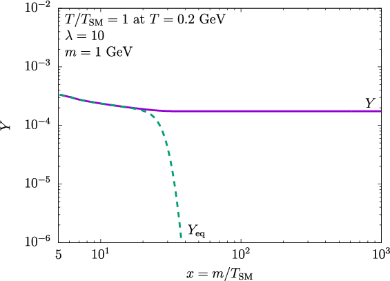
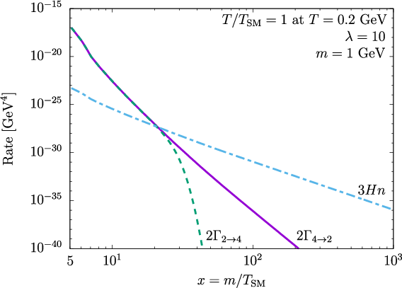
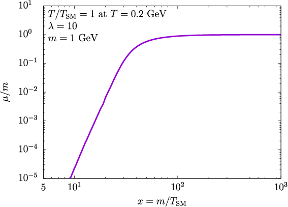
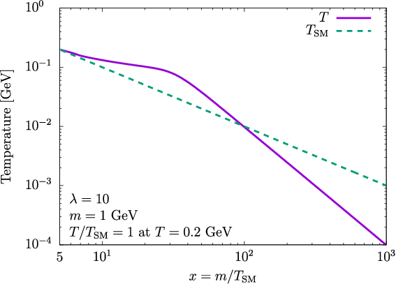
The upper left panel of Fig. 3 shows that $Y(x)$ follows $Y_{\rm eq}$ closely up until $x\sim 25$, at which point it freezes–out and the number density remains approximately constant. As we see from the right upper panel, the freeze–out is well described by

After that, $\Gamma_{4\rightarrow 2}$ becomes suppressed compared to $3nH$, whereas $\Gamma_{2\rightarrow 4}$ turns negligible even faster.

The effective chemical potential becomes appreciable, of order $T$, around the freeze–out point after which it can be approximated by a linear function of $T$ asymptotically approaching $m$, $m-\mu\propto T$. This follows from the entropy and particle number conservation in the dark sector (see Eq. 51). In this regime, $T\propto T_{\rm SM}^{2}$ as required by Eq. 52. Before the freeze–out, the $T$ dependence on $T_{\rm SM}$ is only logarithmic. Non–relativistic behaviour of DM leads to the heating of the dark sector [4], which can be viewed as a result of appreciable $\Gamma_{4\rightarrow 2}$ at that stage.

Note that $Y_{\rm eq}(x)$ is not a solution to the Boltzmann equation since $Y_{\rm eq}^{\prime}(x)$ does not vanish. The true solution $Y(x)$ is close to the “equilibrium” value until freeze–out. This implies that the right hand side of the Boltzmann equation is necessarily non–zero which entails reduction of the total DM number $na^{3}$ during this period. We find that the reaction rate difference $2(\Gamma_{4\rightarrow 2}-\Gamma_{2\rightarrow 4})$ is indeed not far from $3nH$ such that the number reduction is tangible.

After the freeze–out, the particle number is approximately constant, typically within 10%. Hence one can approximate

where $x_{f}$ is the freeze–out point. This is a slightly different condition compared to what is often used in the literature. Here, we do not neglect the $Y_{\rm eq}(x)$ term which makes the number reduction less efficient, especially in the vicinity of the freeze–out point.

For $m/T\lesssim 1$, the relativistic effects are important and one should use the Bose–Einstein distribution function. As Fig. 4 shows, the resulting reaction rates differ from their Maxwell–Boltzmann analogs by $10\%$ to $100\%$ at $m/T\sim 1$, while at $m/T\sim 0.1$ this difference can reach two orders of magnitude. The Bose–Einstein rates are greater due to the enhancement factors for the low energy states. Therefore, the effect is sensitive to the value of the thermal mass and $decreases$ for larger couplings.

As in the non–relativistic case, the evolution of the system is determined by the chemical potential and the temperature. The Boltzmann equation and entropy conservation fix $\mu$ and $T$ as functions of $T_{\rm SM}$. Defining

and $x\equiv m/T_{\rm SM}$, we rewrite the Boltzmann equation as an equation for $\mu(y)$ and $x(y)$:⁶⁶ 6 This can be derived by expressing the left hand side of the Boltzmann equation in terms of $dY/dx$ with $Y=n/s_{\rm SM}$, and calculating this derivative explicitly in terms of $f(p)$.

where

with $E(p)=\sqrt{m^{2}_{\rm eff}+{\bf p}^{2}}\equiv\sqrt{m^{2}+\lambda T^{2}/24+{\bf p}^{2}}$, $n=\int d^{3}{\bf p}/(2\pi)^{3}f(p)$ and $I_{1,2},\Gamma_{2\rightarrow 4}$, $\Gamma_{4\rightarrow 2}$, $\tilde{H},n$ are to be expressed in terms of $\mu,x$ and $y$. The modified Hubble rate $\tilde{H}$ is defined by Eq. 49. Note that we have included the thermal mass correction which leads to an extra contribution in Eq. 60.

The second equation for $\mu(y)$ and $x(y)$ is provided by the entropy conservation condition

with

and $s_{\rm SM}$ from Eq. 46. Here the energy density $\rho$ and the pressure $p$ are given by the standard Bose–Einstein formulas, and are to be expressed in terms of $\mu$ and $y$.

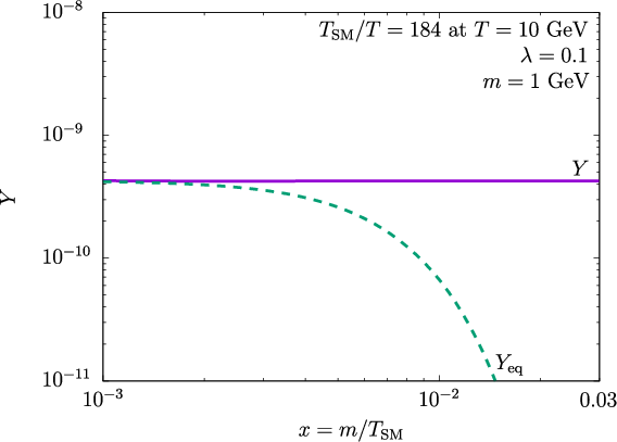
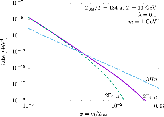
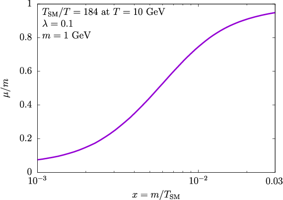
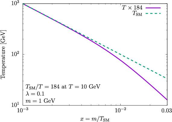
The two coupled equations can be solved numerically.⁷⁷ 7 We compute $\Gamma_{2\rightarrow 4}$ by integrating numerically the CalcHEP output. We present our results in Fig.5. The corresponding freeze–out temperature is $T_{f}=1.2$ GeV with $m=1$ GeV, which makes the freeze–out regime relativistic.

Compared to the non–relativistic case, we observe a few differences. First, the evolution of $Y$ and $\mu$ is slower. Second, there is no “warming” period in which the dark temperature decreases much slower than $T_{\rm SM}$. After freeze–out, $T$ decreases faster than $T_{\rm SM}$ does. This is due to approximate conservation of the particle number $n/T_{\rm SM}^{3}$: the increase in $\mu$ gets compensated by a decrease in $T$. Eventually, $T\propto T_{\rm SM}^{2}$ in the non–relativistic regime. For comparison, we present the evolution of $\xi$ for relativistic and non–relativistic freeze–out in Fig. 6.

Again, we find that $Y(\infty)$ can be well approximated by $Y$ at freeze–out.

Freeze–out at $T\gg m,m/\sqrt{\lambda}$ is not possible in our model. In this regime, $T/T_{\rm SM}$ stays constant by virtue of entropy conservation and

Thus, if the thermal equilibrium condition $3nH<2\Gamma_{2\rightarrow 4}$ is satisfied at some point, it will continue to hold as long as dark matter remains ultra--relativistic.⁸⁸ 8 This is in contrast to the SM neutrino case, where the reaction rate involves a higher power of $T$. As a result, no freeze out is possible.

We note that the thermal mass effect is important in this regime. Due to the infrared singularity, the high temperature rates contain the $T/m_{\rm eff}$ factors. For instance, $\Gamma_{2\rightarrow 2}\propto T^{4}\ln{T\over m_{\rm eff}}\;,$ where $m_{\rm eff}$ includes the thermal correction (36). At $T>5m/\sqrt{\lambda}$, the effective mass is dominated by the thermal term and the expected behaviour $\Gamma_{2\rightarrow 2}\propto T^{4}$ is reproduced. (Here we neglect the usual log–running of the coupling constant which is insignificant for $\lambda$ in the range of interest.) Similar considerations apply to $\Gamma_{2\rightarrow 4}$. The effect of the thermal mass is clearly seen in the left panel of Fig. 7: while in the non–relativistic regime the rate scales as $\lambda^{4}$, at higher temperatures this is no longer true. The $T^{4}$–behaviour is recovered when the thermal mass dominates.

Fig. 7 (right) collects the different regimes in the $\Gamma_{2\rightarrow 4}$ behavior and presents an overall picture. At high temperatures, $\Gamma_{2\rightarrow 4}/n\propto T$ evolves slower than $H\propto T_{\rm SM}^{2}$ does. This changes when the thermal mass becomes subdominant, which is marked as “rel./semi-rel.” in the plot. Finally, in the non–relativistic regime $\Gamma_{2\rightarrow 4}/n\propto n^{3}$ is exponentially suppressed. The magnitude of the rate relative to $H$ is determined by the coupling constant. The plot makes it clear that freeze–out in the ultra–relativistic regime is impossible. Also, if the dashed line is above the solid line, thermalization is never achieved. This is determined by $\Gamma_{2\rightarrow 4}$ in the relativistic/semi–relativistic regime where $T$ is not too far from $m$. The resulting lower bounds on $\lambda$ are presented in Fig. 2.

In this subsection, we assume that dark matter has been in thermal equilibrium and analyze the $(m,\lambda,\xi)$–parameter space consistent with the observed DM relic density. This constraint can be put in the form

Let us discuss the main qualitative features of the model. Consider first the non–relativistic freeze–out regime. As discussed earlier, we define the freeze–out point by

Solving this equation for $T_{f}$ and equating $Y(x_{f})=Y(\infty)$, we find that the correct relic density is reproduced along the curves with the approximate scaling

where $\xi_{f}$ is $T_{\rm SM}/T$ at the freeze–out point and we have neglected the logarithmic terms. For a fixed $\xi_{f}$, the mass–coupling relation is approximately linear and the freeze out temperature decreases with the coupling,

where the constant is positive. Thus, at sufficiently small $\lambda$, the non-relativistic approximation breaks down and a fully relativistic analysis is necessary.

Our numerical results with the relativistic reaction rates are presented in Fig. 8. We observe that in most allowed parameter space the freeze–out is relativistic, i.e. $m/T_{f}<3$ as marked by the green dotted line. In this region, the constant $\xi_{f}$ curves tend to approach a vertical at $T\gtrsim m$ since $Y$ is determined mostly by $\xi$ and rather insensitive to $\lambda$. These curves exhibit characteristic kinks due to a change in the SM degrees of freedom at QCD phase transition ($T_{\rm SM}\sim 10^{-1}$ GeV) and electron decoupling. It is interesting that $T_{f}$ does not vary monotonically along the constant $\xi_{f}$ curve: first, it decreases down to a minimum value and increases from there on.

For a given $\xi_{f}$, the correct relic density curve cannot be continued indefinitely to smaller $\lambda$: at some point, $3nH>2\Gamma_{2\rightarrow 4}$ for any $T$ (see Sec. 4.3). Thus, the relic density and freeze–out equations have no simultaneous solution. The excluded region is marked “no thermalization” in Fig. 8. Although different points on the border of this region correspond to different $\xi$, its shape is consistent with Fig. 2. We note that here the thermal mass effect is significant which makes analytical calculations more challenging.

Another constraint is imposed by the bound on DM self–interaction from the Bullet Cluster, $\sigma/m<1\;{\rm cm^{2}/g}$, with $\sigma=\lambda^{2}/(128\pi m^{2})$. It excludes light DM with significant self–coupling. Finally, perturbative unitarity is violated in the process $SS\rightarrow SS$ if $\lambda\gtrsim 8\pi$ [27]. We note that the nucleosynthesis constraint on the effective number of neutrinos is insignificant here since the dark matter contribution to the energy density in the relativistic regime is suppressed by $T^{4}/T^{4}_{\rm SM}\ll 1$.

In the non–relativistic regime, we find qualitative agreement with the results of Ref. [13] although there are numerical differences.

Fig. 8 shows that the correct relic density can be obtained for a wide range of DM masses: from 10 keV to 100 TeV, as long as the dark temperature is significantly below $T_{\rm SM}$. Thus, both the “warm” and the “cold” options are open.

For small enough self–coupling (see Fig. 2), the system reaches only kinetic but not thermal equilibrium. The notion of temperature is still well defined in this case, but the Bose–Einstein distribution involves an effective chemical potential from the start. The latter is determined by the initial number density. Assuming $T\gg m$, we have

References

- [1] E. Aprile et al. [XENON Collaboration], Phys. Rev. Lett. 121, no. 11, 111302 (2018) doi:10.1103/PhysRevLett.121.111302 [arXiv:1805.12562 [astro-ph.CO]].
- [2] V. Silveira and A. Zee, Phys. Lett. 161B, 136 (1985). doi:10.1016/0370-2693(85)90624-0
- [3] L. J. Hall, K. Jedamzik, J. March-Russell and S. M. West, JHEP 1003, 080 (2010) doi:10.1007/JHEP03(2010)080 [arXiv:0911.1120 [hep-ph]].
- [4] E. D. Carlson, M. E. Machacek and L. J. Hall, Astrophys. J. 398, 43 (1992). doi:10.1086/171833
- [5] P. Gondolo and G. Gelmini, Nucl. Phys. B 360, 145 (1991). doi:10.1016/0550-3213(91)90438-4
- [6] J. McDonald, Phys. Rev. D 50, 3637 (1994) doi:10.1103/PhysRevD.50.3637 [hep-ph/0702143 [HEP-PH]].
- [7] C. P. Burgess, M. Pospelov and T. ter Veldhuis, Nucl. Phys. B 619, 709 (2001) doi:10.1016/S0550-3213(01)00513-2 [hep-ph/0011335].
- [8] A. Djouadi, O. Lebedev, Y. Mambrini and J. Quevillon, Phys. Lett. B 709, 65 (2012) doi:10.1016/j.physletb.2012.01.062 [arXiv:1112.3299 [hep-ph]].
- [9] J. M. Cline, K. Kainulainen, P. Scott and C. Weniger, Phys. Rev. D 88, 055025 (2013) Erratum: [Phys. Rev. D 92, no. 3, 039906 (2015)] doi:10.1103/PhysRevD.92.039906, 10.1103/PhysRevD.88.055025 [arXiv:1306.4710 [hep-ph]].
- [10] J. M. Cornell [GAMBIT Collaboration], PoS ICHEP 2016, 118 (2016) doi:10.22323/1.282.0118 [arXiv:1611.05065 [hep-ph]].
- [11] T. Binder, T. Bringmann, M. Gustafsson and A. Hryczuk, Phys. Rev. D 96, no. 11, 115010 (2017) doi:10.1103/PhysRevD.96.115010 [arXiv:1706.07433 [astro-ph.CO]].
- [12] N. Bernal, C. Garcia-Cely and R. Rosenfeld, JCAP 1504, no. 04, 012 (2015) doi:10.1088/1475-7516/2015/04/012 [arXiv:1501.01973 [hep-ph]].
- [13] N. Bernal and X. Chu, JCAP 1601, 006 (2016) doi:10.1088/1475-7516/2016/01/006 [arXiv:1510.08527 [hep-ph]].
- [14] M. Heikinheimo, T. Tenkanen, K. Tuominen and V. Vaskonen, Phys. Rev. D 94, no. 6, 063506 (2016) Erratum: [Phys. Rev. D 96, no. 10, 109902 (2017)] doi:10.1103/PhysRevD.96.109902, 10.1103/PhysRevD.94.063506 [arXiv:1604.02401 [astro-ph.CO]].
- [15] N. Bernal, M. Heikinheimo, T. Tenkanen, K. Tuominen and V. Vaskonen, Int. J. Mod. Phys. A 32, no. 27, 1730023 (2017) doi:10.1142/S0217751X1730023X [arXiv:1706.07442 [hep-ph]].
- [16] M. Fairbairn, K. Kainulainen, T. Markkanen and S. Nurmi, JCAP 1904, no. 04, 005 (2019) doi:10.1088/1475-7516/2019/04/005 [arXiv:1808.08236 [astro-ph.CO]].
- [17] A. D. Dolgov and K. Kainulainen, Nucl. Phys. B 402, 349 (1993) doi:10.1016/0550-3213(93)90646-7 [hep-ph/9211231].
- [18] P. Adshead, Y. Cui and J. Shelton, JHEP 1606, 016 (2016) doi:10.1007/JHEP06(2016)016 [arXiv:1604.02458 [hep-ph]].
- [19] M. Olechowski and P. L. Szczerbiak, Eur. Phys. J. C 78, no. 9, 704 (2018) doi:10.1140/epjc/s10052-018-6195-0 [arXiv:1807.00490 [hep-ph]].
- [20] J. Bernstein, L. S. Brown and G. Feinberg, Phys. Rev. D 32, 3261 (1985). doi:10.1103/PhysRevD.32.3261
- [21] J. Bernstein, “Kinetic Theory In The Expanding Universe,” doi:10.1017/CBO9780511564185
- [22] E. W. Kolb and M. S. Turner, “The Early Universe,” Front. Phys. 69, 1 (1990).
- [23] K. Enqvist, M. Karciauskas, O. Lebedev, S. Rusak and M. Zatta, JCAP 1611, 025 (2016) doi:10.1088/1475-7516/2016/11/025 [arXiv:1608.08848 [hep-ph]].
- [24] A. K. Das, “Finite Temperature Field Theory,” Singapore, Singapore: World Scientific (1997) 404 pp.
- [25] A. Belyaev, N. D. Christensen and A. Pukhov, Comput. Phys. Commun. 184, 1729 (2013) doi:10.1016/j.cpc.2013.01.014 [arXiv:1207.6082 [hep-ph]].
- [26] M. E. Peskin and D. V. Schroeder, “An Introduction to quantum field theory”, 1997, 842 pp.
- [27] C. Y. Chen, S. Dawson and I. M. Lewis, Phys. Rev. D 91, no. 3, 035015 (2015) doi:10.1103/PhysRevD.91.035015 [arXiv:1410.5488 [hep-ph]].
- [28] H. E. Haber and H. A. Weldon, Phys. Rev. Lett. 46, 1497 (1981). doi:10.1103/PhysRevLett.46.1497
- [29] H. E. Haber and H. A. Weldon, Phys. Rev. D 25, 502 (1982). doi:10.1103/PhysRevD.25.502
- [30] M. Tanabashi et al. [Particle Data Group], Phys. Rev. D 98, no. 3, 030001 (2018). doi:10.1103/PhysRevD.98.030001