Typical properties of interval maps
preserving the Lebesgue measureThanks: We thank the A*MIDEX project (ANR-11-IDEX-0001-02), funded itself by the “Investissements d’avenir” program of the French Government, managed by the French National Research Agency (ANR). The first author was supported by the European Regional Development Fund, project No. CZ 02.1.01/0.0/0.0/16_019/0000778. We thank two anonymous referees as well as Pierre-Antoine Guiheneuf for suggestions which lead to numerous improvement to our exposition.

Jozef Bobok and Serge Troubetzkoy Address: Department of Mathematics of FCE
Czech Technical University in Prague
Thákurova 7, 166 29 Prague 6, Czech Republic Email address: jozef.bobok@cvut.cz Address: Aix Marseille Univ, CNRS, Centrale Marseille, I2M, Marseille, Francepostal address: I2M, Luminy, Case 907, F-13288 Marseille Cedex 9, France Email address: serge.troubetzkoy@univ-amu.fr URL: www.i2m.univ-amu.fr/perso/serge.troubetzkoy/

Abstract.

We consider the class of the continuous functions from $[0,1]$ into itself which preserve the Lebesgue measure. This class endowed with the uniform metric constitutes a complete metric space. We investigate the dynamical properties of typical maps from the space.

Key words and phrases:

weakly mixing, leo, entropy

2000 Mathematics Subject Classification

37E05, 37B40, 46B25, 46.3

1. Introduction and summary of results

This article is about typical properties of continuous maps of the interval which preserve the Lebesgue measure. Throughout the article the word typical will mean that with respect to the uniform topology there is a dense $G_{\delta}$ set of maps having this property. Such results are in the domain of approximation theory. To our knowledge, the use of approximation techniques in dynamical systems was started in 1941 by Oxtoby and Ulam who considered a simplicial polyhedron with a non-atomic measure which is positive on open sets. In this setting they showed that the set of ergodic measure-preserving homeomorphisms is typical in the strong topology [32]. In 1944 Halmos introduced approximation techniques in a purely metric situation: the study of invertible mode 0 maps of the interval $[0,1]$ which preserve the Lebesgue measure. He showed that the typical invertible map is weakly mixing, i.e., has continuous spectrum [19],[20],[21]. In 1948 Rohlin showed that the set of (strongly) mixing measure preserving invertible maps is of the first category [29]. In 1967 Katok and Stepin [24] introduced the notation of speed of approximation. One of the notable applications of their method is the typicality of ergodicity and weak mixing for certain classes of interval exchange transformations. Katok has shown that interval exchange transformations are never mixing [23].

The study of typical properties of homeomorphism of compact manifolds which preserve regular measures was continued and generalized by Katok and Stepin in 1970 [25] who showed the typicality of ergodicity, of simple continuous spectrum, and the absence of mixing. In 1980 Yano showed that the generic homeomorphism of a compact manifold has infinite entropy [35]. More recently Alpern and co-authors have unified the studies of homeomorphisms and of measure preserving transformations and shown that if a property is typical for measure preserving transformations then it is typical for homeomorphisms [3], [2], [4]. Recently many authors have shown that that the shadowing property is generic in various setting: [12], [18], [26], [27],[33].

Except for Yano’s result which also holds for generic continuous maps of compact manifolds, all of these results are about invertible maps. The measure theoretic properties of $C^{0}$ -generic systems on compact manifolds have first been studied by Abdenur and Andersson [1]; their main result is that a $C^{0}$ -generic map has no physical measure, however the Birkhoff average of any continuous function is convergent for Lebesgue a.e. point. Catsigeras and Troubetzkoy gave a quite detailed description of the invariant measures of $C^{0}$ generic continuous maps of compact manifolds with or without boundary (as well as for generic homeomorphisms in the same setting) [13], [14], [15].

Many more more details of the history of approximation theory can be found in the surveys [16], [7].

In this article we consider the set $C(\lambda)$ if continuous non-invertible maps of the unit interval $[0,1]$ which preserve the Lebsegue measure $\lambda$ . Every such map has a dense set of periodic points. Furthermore, except for the two exceptional maps $id$ and $1-id$ , every such map has positive metric entropy. The $C(\lambda)$ -typical function (all the properties will be defined later in the article):

(i)

is weakly mixing with respect to $\lambda$ (Theorem 15),
(ii)

is leo (Theorem 9),
(iii)

satisfies the periodic specification property (Corollary 10)
(iv)

has a knot point at $\lambda$ almost every point [11],
(v)

maps a set of Lebesgue measure zero onto $[0,1]$ (Corollary 22),
(vi)

has infinite topological entropy (Proposition 26),
(vii)

has Hausdorff dimension = lower Box dimension = 1 $<$ upper Box dimension = 2 [31].

Furthermore, in analogy to Rohlin’s result, we show that the set of mixing maps in $C(\lambda)$ is dense (Corollary 14) and of the first category (Theorem 20). We also show that for any $c>0$ as well as for $c=\infty$ the set of maps having metric entropy $c$ is dense in $C(\lambda)$ , however, we do not know if there is a value $c$ such that this set is generic.

Points i) and vi) and the furthermore results are analogous to results in the invertible case, and the proofs of these results follow the same general plan as in the invertible case. The other points have no analogies in the invertible case

Let $\mu$ be a probability Borel measure with full support, let $C(\mu)$ be the set of all continuous interval maps preserving the measure $\mu$ equipped with the uniform metric. The map $h\colon~[0,1]\to[0,1]$ defined as $h(x)=\mu([0,x])$ for $x\in[0,1]$ , is a homeomorphism of $[0,1]$ . In fact, in this settings $\lambda=h^{*}\mu$ , i.e., $\lambda$ is the pushforward measure of $\mu$ by $h$ . Moreover, the map $H\colon~C(\lambda)\to C(\mu)$ given by $f\longmapsto h^{-1}\circ f\circ h$ is a homermoprhism of the spaces $C(\lambda)$ and $C(\mu)$ . Using $H$ , we can transfer the properties (i)-(vi) listed above into the context of $C(\mu)$ . In particular, the property (iv) in $C(\mu)$ says that $C(\mu)$ -typical function has a knot point at $\mu$ almost every point [11].

2. Maps in $C(\lambda)$

Let $\lambda$ denote the Lebesgue measure on $[0,1]$ and ${\mathcal{B}}$ the Borel sets in $[0,1]$ . Let $C(\lambda)$ consist of all continuous $\lambda$ -preserving functions from $[0,1]$ onto $[0,1]$ , i.e.,

C(\lambda)=\{f\colon~[0,1]\to[0,1]\colon~\forall A\in{\mathcal{B}},~\lambda(A)=\lambda(f^{-1}(A))\}.

We consider the uniform metric $\rho$ on $C(\lambda)$ : $\rho(f,g):=\sup_{x\in[0,1]}|f(x)-g(x)|$ .

Proposition 1.

$(C(\lambda),\rho)$ is a complete metric space.

We leave the standard proof of this result to the reader.

Definition 2.

We say that continuous maps $f,g\colon~[a,b]\subset[0,1]\to[0,1]$ are $\lambda$ -equivalent if for each Borel set $A\in{\mathcal{B}}$ ,

\lambda(f^{-1}(A))=\lambda(g^{-1}(A)).

For $f\in C(\lambda)$ and $[a,b]\subset[0,1]$ we denote by $C(f;[a,b])$ the set of all continuous maps $\lambda$ -equivalent to $f\upharpoonright[a,b]$ . We define

C_{*}(f;[a,b]):=\{h\in C(f;[a,b])\colon~h(a)=f(a),~h(b)=f(b)\}.

Definition 3.

Let $f$ be from $C(\lambda)$ and $[a,b]\subset[0,1]$ . For any fixed $m\in{\mathbb{N}}$ , let us define the map $h=h\langle f;[a,b],m\rangle\colon~[a,b]\to[0,1]$ by $j\in\{0,\dots,m-1\}$ and

(1)

h(a+x):=\begin{cases}f\left(a+m\Big(x-\frac{j(b-a)}{m}\Big)\right)\text{ if }x\in\left[\frac{j(b-a)}{m},\frac{(j+1)(b-a)}{m}\right],~j\text{ even},\\ f\left(a+m\Big(\frac{(j+1)(b-a)}{m}-x\Big)\right)\text{ if }x\in\left[\frac{j(b-a)}{m},\frac{(j+1)(b-a)}{m}\right],~j\text{ odd}.\end{cases}

Then $h\langle f;[a,b],m\rangle\in C(f;[a,b])$ for each $m$ and $h\langle f;[a,b],m\rangle\in C_{*}(f;[a,b])$ for each $m$ odd .

Example 4.

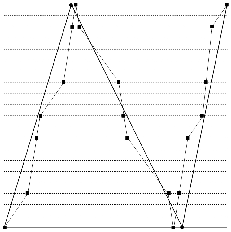
In Figure 1, for $f\in C(\lambda)$ shown on the left, on the right we show the regular $3$ -fold window perturbation of $f$ by $h=h\langle f;[a,b],3\rangle\in C_{*}(f;[a,b])$ .

Figure 1. The map

g

3

-fold regular window perburbation of the map

f

For a fixed $h\in C_{*}(f;[a,b])$ , the map $g=g\langle f,h\rangle\in C(\lambda)$ defined by

(2)

g(x):=\begin{cases}f(x)\text{ if }x\notin[a,b],\\ h(x)\text{ if }x\in[a,b]\end{cases}

will be called the window perturbation of $f$ (by $h$ on $[a,b]$ ). In particular, if $h=h\langle[f;[a,b],m\rangle$ , $m$ odd, resp. $h$ is piecewise affine, we will speak of regular $m$ -fold, resp. piecewise affine window perturbation $g$ of $f$ (on $[a,b]$ ) - see Figure 1.

The following useful observation will be repeatedly used in our text. We will omit its proof since it is a straightforward consequence of the uniform continuity of $f$ .

Lemma 5.

Let $f$ be from $C(\lambda)$ . For each $\varepsilon>0$ there is $\delta>0$ such that

(3)

\forall~[a,b]\subset[0,1],~b-a<\delta~\forall~h\in C_{*}(f;[a,b])\colon~\rho(f,g\langle f,h\rangle)<\varepsilon.

In particular, for each $\varepsilon>0$ there is a positive integer $n_{0}>0$ such that for each $n>n_{0}$ , if $I_{j}=[\frac{j}{n},\frac{(j+1)}{n}]$ and

g\upharpoonright I_{j}=h\langle f;I_{j},m(j)\rangle

with odd numbers $m(j)$ for every $j\in\{0,\dots,n-1\}$ , then $\rho(f,g)<\varepsilon$ independently of the numbers $m(j)$ .

Below we introduce three classical types of mixing in topological dynamics. We consider them in the context of $C(\lambda)$ .

A map $f\in C(\lambda)$ is called

•

transitive if for each pair of nonempty open sets $U,V$ , there is $n\geqslant 0$ such that $f^{n}(U)\cap V\neq\emptyset$ ,
•

topologicalyl mixing if for each pair of nonempty open sets $U,V$ , there is $n_{0}\geq 0$ such that $f^{n}(U)\cap V\neq\emptyset$ for every $n\geqslant n_{0}$ ,
•

leo (locally eventually onto) if for every nonempty open set $U$ there is $n\in{\mathbb{N}}$ such that $f^{n}(U)=[0,1]$ .

For each map $f\in C(\lambda)$ the set of periodic points is dense in $[0,1]$ , this is a consequence of the Poincaré Recurrence Theorem and the fact that in dynamical system given by an interval map the closures of recurrent points and periodic points coincide [17]. Thus Proposition 6 and Lemma 7, stated below, apply to elements of $C(\lambda)$ .

For two intervals $J_{1},J_{2}$ with pairwise disjoint non-empty interiors we write $J_{1}<J_{2}$ if $x_{1}<x_{2}$ for some points $x_{1}\in J_{1}$ and $x_{2}\in J_{2}$ . Throughout the article we will denote the interior of an interval $J$ by the notation $J^{\circ}$ .

Figure 2.

f,g\in C(\lambda)

; Prop. 6(5):

{\mathcal{J}}(f)=\{J_{i}\}_{i=1}^{5}

f(J_{1})=J_{5}

f(J_{2})=J_{4}

f(J_{3})=J_{3}

f(J_{4})=J_{2}

f(J_{5})=J_{1}

; Prop. 6(4):

{\mathcal{J}}(g)=\{J_{i}\}_{i=1}^{5}

g(J_{i})=J_{i}

for each

i

Proposition 6.

[6] Suppose $f$ has a dense set of periodic points. The following assertions hold (Figure 2).

(i)

There is a collection (perhaps finite or empty) ${\mathcal{J}}={\mathcal{J}}(f)=\{J_{1},J_{2},\dots\}$ of closed subintervals of $[0,1]$ with mutually disjoint interiors, such that for each $i$ , $f^{2}(J_{i})=J_{i}$ , and there is a point $x_{i}\in J_{i}$ such that $\{f^{4n}(x_{i})\colon~n\geqslant 0\}$ is dense in $J_{i}$ .
(ii)

If $\#{\mathcal{J}}\geqslant 2$ then either

(4) $\forall~J_{1},J_{2}\in{\mathcal{J}}\colon~J_{1}<J_{2}\implies f(J_{1})<f(J_{2})$

or

(5) $\forall~J_{1},J_{2}\in{\mathcal{J}}\colon~J_{1}<J_{2}\implies f(J_{1})>f(J_{2}).$
(iii)

For each $J\in{\mathcal{J}}$ , $f(J)\in{\mathcal{J}}$ and $f^{-1}(f(J))=J$ .
(iv)

If (4) is true then $f(J)=J$ for each $J\in{\mathcal{J}}$ .
(v)

If (5) holds true $f(J)=J$ if and only if $J^{\circ}\cap{\hbox{{\rm Fix}}}(f)\neq\emptyset$ and there is at most one such interval.
(vi)

If $x\in(0,1)\setminus\bigcup_{i\geqslant 1}J_{i}^{\circ}$ , then $f^{2}(x)=x$ .
(vii)

For each $J\in{\mathcal{J}}$ , the map $f^{2}\upharpoonright J$ is topologically mixing.
(viii)

For each $J\in{\mathcal{J}}$ , if $f(J)=J$ then the map $f\upharpoonright J$ is topologically mixing.
(ix)

The map $f$ is surjective.

Proof.

Properties (i)-(vi) had been proved in [6]. The other ones easily follow.
(vii) It is well known that an interval map $g\colon~J\to J$ is topologically mixing if and only if $g^{2}$ is transitive [8, Theorem 46]. By (i), the set $\{f^{4n}(x)\colon~n\geqslant 0\}$ is dense in $J$ for some $x\in J$ , hence $f^{4}\upharpoonright J$ is transitive, i.e., $f^{2}\upharpoonright J$ is topologically mixing.
(viii) From (vii) we know that $f^{2}\upharpoonright J$ is topologically mixing hence also transitive and as in (vii) we can deduce that $f\upharpoonright J\colon~J\to J$ is topologically mixing.
(ix) Since $f$ is continuous, the image $f([0,1])$ is a closed interval and by our assumption it contains a dense subset of $[0,1]$ , so $f([0,1])=[0,1]$ . ∎

Lemma 7.

Suppose $f$ has a dense set of periodic points.

(i)

The map $f$ is transitive but not topologically mixing if and only if ${\mathcal{J}}=\{[0,b],[b,1]\}$ and $f([0,b])=[b,1]$ .
(ii)

The map $f$ is topologically mixing if and only if ${\mathcal{J}}=\{[0,1]\}$ .
(iii)

The map $f$ is leo if and only if ${\mathcal{J}}=\{[0,1]\}$ and both of the sets $f^{-2}(0)\cap(0,1)$ and $f^{-2}(1)\cap(0,1)$ are non-empty.

Proof.

Parts (i) and (ii) follow immediately from Proposition 6, thus we begin by the only if direction of (iii).

By (ii), if ${\mathcal{J}}\neq\{[0,1]\}$ then $f$ is not topologically mixing, and thus not leo, thus we suppose ${\mathcal{J}}=\{[0,1]\}$ . Suppose first that $f^{-2}(0)\cap(0,1)=\emptyset$ . The leo map $f$ is continuous and surjective hence every point in $(0,1)$ must have at least one preimage in $(0,1)$ . This fact and our assumption $f^{-2}(0)\cap(0,1)=\emptyset$ imply $f^{-1}(0)\subset\{0,1\}$ .

If $f(1)\neq 0$ then $f^{-1}(0)=\{0\}$ and $0\notin f^{n}((0,1])$ for every $n$ positive. If $f(1)=0$ then by our assumption, $f^{-1}(1)\cap(0,1)=\emptyset$ hence $f(0)=1$ . It implies that $f^{2}(0)=0$ , $f^{2}(1)=1$ and $0\notin f^{2n}((0,1])$ , what contradicts the leo property of $f$ . The case when $f^{-2}(1)\cap(0,1)=\emptyset$ can be proven analogously.

We turn to the if direction. We assume that ${\mathcal{J}}=\{[0,1]\}$ and that $f^{-2}(0)\cap(0,1)\neq\emptyset\neq f^{-2}(1)\cap(0,1)=\emptyset$ ; since by (ii) $f$ is topologically mixing, for every nonempty open $L\subset[0,1]$ there has to exist a positive $n$ for which $f^{n}(L)\cap f^{-2}(0)\neq\emptyset\neq f^{n}(L)\cap f^{-2}(1)$ hence $f^{n+2}(L)=[0,1]$ . ∎

For any set $X\subset C([0,1])$ we denote by $X_{property}$ the set of all maps in $X$ having a property (in lower index abbreviated) in question. We denote by $PA(\lambda)$ the set of all piecewise affine maps from $C(\lambda)$ .

Proposition 8.

The set $PA(\lambda)_{leo}$ is dense in $C(\lambda)$ .

Proof.

Fix an $f\in C(\lambda)$ and $\varepsilon>0$ . It had been shown in [11] that there exists a map $d^{\star}\in PA(\lambda)$ such that $\rho(d^{\star},f)<\varepsilon$ .

Let us show with the help of Lemma 5 that there exists a map $d^{\star\star}\in PA(\lambda)_{leo}$ for which $\rho(d^{\star\star},d^{\star})<\varepsilon$ . First we prove
Claim. $PA(\lambda)_{leo}=PA(\lambda)_{tmix}$ .
Proof of Claim. Any leo map is topologically mixing. So let $f\in PA(\lambda)_{tmix}$ and show that $f\in PA(\lambda)_{leo}$ . If $f^{-1}(0)\cap(0,1)=f^{-1}(1)\cap(0,1)=\emptyset$ , then since $f$ is surjective either $f^{-1}(0)=\{0\}$ , $f^{-1}(1)=\{1\}$ or $f^{-1}(0)=\{1\}$ and $f^{-1}(1)=\{0\}$ . But $f\in C(\lambda)$ , so $f^{\prime}\equiv 1$ on some neighborhood of $\{0,1\}$ in the first case or $f^{\prime}\equiv-1$ on some neighborhood of $\{0,1\}$ in the latter case - a contradiction with topological mixing of $f$ . So assume that $f^{-1}(0)\cap(0,1)\neq\emptyset$ . As in the proof of Lemma 7, since $f$ is continuous and surjective, $f^{-2}(0)\cap(0,1)\neq\emptyset$ and by Lemma 7(iii), it is sufficient to show that $f^{-2}(1)\cap(0,1)\neq\emptyset$ , resp. $f^{-1}(1)\cap(0,1)\neq\emptyset$ . Let $f^{-1}(1)\cap(0,1)=\emptyset$ . We are done if $\{0\}\subset f^{-1}(1)$ , since then $f^{-2}(1)\cap(0,1)\cap f^{-1}(0)\neq\emptyset$ . It remains to comment the case $f^{-1}(1)=\{1\}$ . Then since $f\in C(\lambda)$ , $f^{\prime}\equiv 1$ on some neighborhood of $1$ - a contradiction with topological mixing of $f$ . The case when $f^{-1}(1)\cap(0,1)\neq\emptyset$ can be captured analogously. This finishes the proof of the claim.

By our claim we are done if $d^{\star}\in PA(\lambda)_{tmix}$ , so assume that this is not the case. Notice that since $d^{\star}$ is piecewise affine, the set ${\mathcal{J}}(d^{\star})$ is a finite set, ${\mathcal{J}}(d^{\star})=\{J_{i}\colon~i=1,\dots,k\}$ with $2\leqslant k<\infty$ , and thus the set $[0,1]\setminus\bigcup{\mathcal{J}}(d^{\star})$ has a finite number of connected components, each one is an interval. Without loss of generality we can assume that each of these intervals is reduced to a single point (if it were not the case, we could use Proposition 6 and a finite number of regular $m$ -fold, $m\geqslant 3$ , piecewise affine window perturbations on a finite collection of sufficiently small adjacent subintervals of those connected components as described in Lemma 5 - see Figure 3(Left)). Let $J=[a,b]$ and $J^{\prime}=[b,c]$ be two adjacent element of ${\mathcal{J}}(d^{\star})$ - see Figure 3(Right).

Figure 3. Left:

f\in C(\lambda)

\bigcup{\mathcal{J}}(f)=\bigcup\{J_{i}\}_{i=1}^{2}

is not dense, regular

3

-fold perturbations of

f

on new

J

’s; Right: Perturbation on

U_{1}(b)

and

U_{2}(b)\subset U_{1}(b)

from the proof of Prop. 8.

•

Using a piecewise affine window perturbation (not necessarily regular) on some neighborhood of $b$ if necessary, w.l.o.g. we can assume that $d^{\star}$ is strictly monotone with a constant slope on neighborhood $U_{1}(b)$ of $b$ .
•

Choosing sufficiently small $\varepsilon_{1}<\varepsilon$ we can consider the regular $3$ -fold window perturbation of $d^{\star}$ on $U_{2}(b)\subset U_{1}(b)$ resulting in the map $d^{\star}_{1}\in PA(\lambda)$ satisfying $\rho(d^{\star},d^{\star}_{1})<\varepsilon_{1}$ . Moreover, by Proposition 6 and Lemma 7 either

- $\#{\mathcal{J}}(d^{\star}_{1})=k-1<\#{\mathcal{J}}(d^{\star})=k$ in the case of Equation (4), resp. Equation (5) with $b\in{\hbox{{\rm Fix}}}(f)$ or

- $\#{\mathcal{J}}(d^{\star}_{1})=k-2<\#{\mathcal{J}}(d^{\star})=k$ in the case of Equation (5) with $b\notin{\hbox{{\rm Fix}}}(f)$ .

Finitely many modifications of $d^{\star}$ with $\varepsilon_{1},\dots,\varepsilon_{\ell}$ , $\ell\leqslant k-1$ , satisfying

\varepsilon_{1}+\cdots+\varepsilon_{\ell}<\varepsilon

result to maps $d^{\star}_{1},\dots,d^{\star}_{\ell}$ for which

\rho(d^{\star}_{i},d^{\star}_{i+1})<\varepsilon_{i+1},\quad i\in\{1,\dots,\ell-1\},

$d^{\star}_{\ell}\in C(\lambda)$ , $\#{\mathcal{J}}(d^{\star}_{\ell})=1$ , and

\rho(d^{\star},d^{\star}_{\ell})<\varepsilon_{1}+\sum_{i=1}^{\ell-1}\rho(d^{\star}_{i},d^{\star}_{i+1})<\varepsilon.

Summarizing, from Lemma 7(iii) we obtain that $d^{\star\star}=d^{\star}_{\ell}$ is topologically mixing hence also from $PA(\lambda)_{leo}$ and $\rho(d^{\star\star},f)<2\varepsilon$ . ∎

Theorem 9.

The $C(\lambda)$ -typical function is leo.

Proof.

By Proposition 8 we can fix a countable dense collection $\{f_{n}\}_{n}$ from $PA(\lambda)_{leo}$ . Using a $2$ -fold piecewise affine window perturbation of $f_{n}$ on $[0,\varepsilon]$ , resp. $[1-\varepsilon,1]$ if necessary - see Example 3 and Lemma 5 - without loss of generality we can assume that for each $n\in{\mathbb{N}}$ we have $f_{n}(0)\in(0,1)$ and $f_{n}(1)\in(0,1)$ .

Let $B(g,\varepsilon):=\{f\in C(\lambda):\rho(f,g)<\varepsilon\}$ . For a given sequence $\{\varepsilon_{n}:\varepsilon_{n}>0\}_{n}$ which we will choose later, we consider the dense $G_{\delta}$ set

G:=\bigcap_{N\geqslant 1}\bigcup_{n\geqslant N}B(f_{n},\varepsilon_{n}).

We claim that we can choose $\varepsilon_{n}$ in such a way that any $f\in G$ is leo.

Consider a sequence $(J_{m})_{m\in{\mathbb{N}}}$ of all open rational subintervals of $(0,1)$ . For each $n,m$ there is a $j(n,m)\in{\mathbb{N}}$ such that $f_{n}^{j(n,m)}(J_{m})=[0,1]$ . Choose $\varepsilon_{n}>0$ so small so that for all $f\in B(f_{n},\varepsilon_{n})$ we have $f^{j(n,m)}(J_{m})\supset(1/n,1-1/n)$ for $m=1,2,\dots,n$ . Additionally we assume that $\varepsilon_{n}>0$ is so small that $f(0)\in(0,1)$ and $f(1)\in(0,1)$ .

Now consider an $f\in G$ . Then there exists an infinite sequence $(n_{k})_{k\in{\mathbb{N}}}$ so that $f\in B(f_{n_{k}},\varepsilon_{n_{k}})$ . By Proposition 6(ix) the map $f$ is surjective. Thus there are points $a,b\in[0,1]$ such that $f(a)=0$ and $f(b)=1$ . By the choice of $\varepsilon_{n}$ we have such points $a,b\in(0,1)$ .

Fix an open interval $J\subset[0,1]$ . Choose an $m$ so that $J_{m}\subset J$ . Suppose $n_{k}$ satisfies the following conditions (i) $n_{k}\geqslant m$ and (ii) $a,b\in(1/n_{k},1-1/n_{k})$ . Assume $a<b$ , the other case being similar. By construction of $G$ and the above two assumptions we have

f^{j(n_{k},m)}(J)\supset f^{j(n_{k},m)}(J_{m})\supset(1/n_{k},1-1/n_{k})\supset[a,b].

Thus $f^{j(n_{k},m)+1}(J)\supset f([a,b])=[0,1].$ ∎

For integers $a\geqslant b\geqslant 0$ let $f^{[a,b]}(x):=\{f^{j}(x):a\leqslant j\leqslant b\}$ . A family of orbit segments $\{f^{[a_{j},b_{j}]}(x_{j})\}_{j=1}^{n}$ is an $N$ -spaced specification if $a_{i}-b_{i-1}\geqslant N$ for $2\leqslant i\leqslant n$ . We say that a specification $\{f^{[a_{j},b_{j}]}(x_{j})\}_{j=1}^{n}$ is $\varepsilon$ -shadowed by $y\in[0,1]$ if

d(f^{k}(y),f^{k}(x_{i}))\leqslant\varepsilon\text{ for }a_{i}\leqslant k\leqslant b_{i}\text{ and }1\leqslant i\leqslant n.

We say that $f$ has the specification property if for any $\varepsilon>0$ there is a constant $N=N(\varepsilon)$ such that any $N$ -spaced specification $\{f^{[a_{j},b_{j}]}(x_{j})\}_{j=1}^{n}$ is $\varepsilon$ -shadowed by some $y\in[0,1]$ . If additionally, $y$ can be chosen in such a way that $f^{b_{n}-a_{0}+N}(y)=y$ then $f$ has the periodic specification property.

Applying a result of Blokh [10] we obtain

Corollary 10.

The $C(\lambda)$ -typical function satisfies the periodic specification property.

3. Mixing properties in $C(\lambda)$

We start by introducing three classical types of mixing in a measure-theoretical dynamics [34]. We state them in the context of $C(\lambda)$ .

Definition 11.

A map $f\in C(\lambda)$ is called

(i)

ergodic, if for every $A,B\in{\mathcal{B}}$ ,

$\lim_{n\to\infty}\frac{1}{n}\sum_{j=0}^{n-1}\lambda(f^{-j}(A)\cap B)=\lambda(A)\lambda(B).$
(ii)

weakly mixing, if for every $A,B\in{\mathcal{B}}$ ,

$\lim_{n\to\infty}\frac{1}{n}\sum_{j=0}^{n-1}|\lambda(f^{-j}(A)\cap B)-\lambda(A)\lambda(B)|=0.$
(iii)

strongly mixing, if for every $A,B\in{\mathcal{B}}$ ,

$\lim_{n\to\infty}\lambda(f^{-j}(A)\cap B)=\lambda(A)\lambda(B).$

Analogously as before, for a subset $X\subset C(\lambda)$ we denote by $X_{slope>1}$ the set of all maps $f$ from $X$ for which $|f^{\prime}(x)|>1$ for all $x\in[0,1]$ at which derivative of $f$ exists.

We denote by $PAM(\lambda)$ the set of all piecewise affine Markov maps in $PA(\lambda)$ , i.e., maps for which all points of discontinuity of the derivative and also both endpoints $0,1$ are eventually periodic.

Proposition 12.

The set $PAM(\lambda)_{leo}$ is dense in $C(\lambda)$ .

Proof.

Let $f\in PA(\lambda)_{leo}$ , fix $\varepsilon>0$ . Denote $R(f)$ the set containing $\{0,1\}$ and all points of discontinuity of the derivative of $f$ , let $S(f)\subset R(f)$ be eventually periodic points from $R(f)$ and $T(f)=R(f)\setminus S(f)$ .

Clearly the set $R(f)$ is finite. Fix $t\in T=T(f)$ . By Proposition 6(ix) and Lemma 5 we can consider a periodic orbit $P=\{p_{1}<\cdots<p_{k}\}$ of $f$ such that for some three consecutive points $p_{i-1}<p_{i}<p_{i+1}$

•

$f\upharpoonright[p_{i-1},p_{i+1}]$ is affine,
•

$\mbox{\rm orb}(S(f),f)\cap[p_{i-1},p_{i+1}]=\emptyset$ ,
•

every window perturbation of $f$ by $h\in C(f;[p_{i-1},p_{i+1}])$ on $[p_{i-1},p_{i+1}]$ is $\varepsilon/m$ -close to $f$ , where $m=\#T$ ,
•

every piecewise affine window perturbation of $f$ on $[p_{i-1},p_{i+1}]$ belongs to $PA(\lambda)_{leo}$ ,
•

$\mbox{\rm orb}(t,f)\cap(p_{i-1},p_{i+1})\neq\emptyset$ .

Let $f^{\ell}(t)$ be the first iterate of $t$ in $(p_{i-1},p_{i+1})$ . By Lemma 5 there exists a $5$ -fold piecewise affine window perturbation (not necessarily regular) $g_{1}$ of $f$ by $h$ on $[p_{i-1},p_{i+1}]$ satisfying

g_{1}(f^{\ell}(t))=g_{1}(p_{i})=f(p_{i}).

Then $\#R(g_{1})=\#R(f)+6$ and $\#S(g_{1})\geqslant\#S(f)+7$ hence

		$\displaystyle\#T(f)-1=m-1=\#R(f)+6-(\#S(f)+7)\geqslant$
		$\displaystyle\geqslant\#R(g_{1})-\#S(g_{1})=\#T(g_{1}).$

Repeating the above procedure maximally $m=\#T$ -times, we obtain the required Markov map $g\in PAM(\lambda)_{leo}$ . ∎

Let $f$ be from $PAM(\lambda)_{slope>1}$ with a Markov partition

{\mathcal{A}}=\{A_{0}=[x_{0},x_{1}]\leqslant\cdots\leqslant A_{N-1}=[x_{N-1},x_{N}]\},

where the set $P_{f}=\{0=x_{0}<\cdots<x_{N}=1\}$ contains orbits of all points of discontinuity of derivative of $f$ and of the endpoints. To each point $x\in[0,1]$ we associate its itinerary $\Phi(x)=(\phi_{i}(x))_{i\geqslant 0}$ with respect to ${\mathcal{A}}$ , i.e., $\phi_{i}(x)\in\{0,1,\dots,N-1\}$ and $f^{i}(x)\in A_{\phi_{i}(x)}$ for each $i\geqslant 0$ (in this settings $\Phi$ is a one-to-finite multivalued map). Since $f$ is continuous, the system $(\Phi([0,1]),\sigma)$ is a subshift of the full shift $(\{0,1,\dots,N-1\}^{{\mathbb{N}}_{0}},\sigma)$ on the symbols $\{0,1,\dots,N-1\}$ [34].

Any map from $PAM(\lambda)_{leo}$ satisfies the hypothesis of [5, Theorem 3.2]. So any such map is in fact exact, i.e., for every $A\in\bigcap_{n\geqslant 0}T^{-n}({\mathcal{B}})$ , $\lambda(A)\lambda(A^{c})=0$ . It is known that every exact map has one-sided countable Lebesgue spectrum and hence is strongly mixing [34, p. 115]. For our purpose it will be convenient to prove explicitly the following.

Lemma 13.

Let $f$ be from $PAM(\lambda)_{slope>1}$ , consider ${\mathcal{A}}$ and $\Phi$ as above. The system $([0,1],{\mathcal{B}},\lambda,f)$ is isomorphic to the one-sided Markov shift $(\Phi([0,1])),{\mathcal{B}}^{\prime},\mu,\sigma)$ , where the measure $\mu$ on the Borel $\sigma$ -algebra ${\mathcal{B}}^{\prime}$ is given by the probability vector

(6)

p=(\lambda(A_{0}),\dots,\lambda(A_{N-1}))

and the stochastic matrix $P=\left(p_{ij}\right)_{i,j=0}^{N-1}$ , where

(7)

p_{ij}=\begin{cases}\frac{\lambda(A_{j})}{\lambda(f(A_{i}))},&f(A_{i})\supset A_{j}\\ 0,&\text{otherwise}\end{cases}.

In particular every map from $PAM(\lambda)_{leo}$ is strongly mixing.

Proof.

For the definition of isomorphic measure theoretic systems see [34, Definition 2.4]. Clearly, the vector $p$ is a probability vector and, since $f\in C(\lambda)$ with constant derivative on each $A_{i}$ , the matrix $P$ is stochastic and $pP=p$ . So the measure $\mu$ is defined well on the Borel $\sigma$ -algebra ${\mathcal{B}}^{\prime}$ generated by the cylinders in $\Phi([0,1])$ . Since $f\in PAM(\lambda)_{slope>1}$ , $\Phi$ is injective. Let $N$ be the set of those points $x$ from $[0,1]$ for which the set $\Phi(x)$ consists of more itineraries. Then $N$ is countable and, since $\Phi$ is a one-to-finite multivalued map, the set $\Phi(N)$ is also countable. Hence $\Phi\colon~[0,1]\setminus N\to\Phi([0,1]\setminus N)$ is a bijection and $\lambda([0,1]\setminus N)=\mu(\Phi([0,1]\setminus N))=1$ . Obviously,

\Phi\circ f=\sigma\circ\Phi\text{ on }[0,1]\setminus N.

To finish the proof we need to show that

\lambda(\Phi^{-1}(A))=\mu(A)\text{ for each }A\in{\mathcal{B}}^{\prime}.

Obviously it is sufficient to verify the last equality for cylinders, i.e., the sets

C_{\phi_{0},\dots,\phi_{k-1}}=\{(\phi_{i}(x))_{i\geqslant 0}\in\phi([0,1])\colon~\phi_{0}(x)=\phi_{0},\dots,\phi_{k-1}(x)=\phi_{k-1}\},

where $k\in{\mathbb{N}}$ and $\phi_{0},\dots,\phi_{k-1}\in\{0,\dots,N-1\}$ . By the definition of the Markov shift

\mu(C_{\phi_{0},\dots,\phi_{k-1}})=\lambda(A_{\phi_{0}})\prod_{j=1}^{k-1}\frac{\lambda(A_{\phi_{j}})}{\lambda(f(A_{\phi_{j-1}}))}=\clubsuit,

where the second factor equals to one if $k=1$ . Since $f$ has a constant derivative on each $A_{i}$ ,

\clubsuit=\lambda(\Phi^{-1}(C_{\phi_{0},\dots,\phi_{k}})).

If $f\in PAM(\lambda)_{leo}\cap PAM(\lambda)_{slope>1}$ , the matrix $P$ is irreducible and aperiodic, hence

(\Phi([0,1])),{\mathcal{B}}^{\prime},\mu,\sigma)

is strogly mixing [34, Theorem 1.31]. By the previous, it is also true for isomorphic $([0,1],{\mathcal{B}},\lambda,f)$ . ∎

Corollary 14.

The set $C(\lambda)_{smix}$ of strongly mixing maps is dense in $C(\lambda)$ .

Proof.

It is a consequence of Proposition 12 and Lemma 13. ∎

Theorem 15.

$C(\lambda)$ -typical function is weakly mixing.

Proof.

By Proposition 12 and Lemma 13 we can consider a countable dense set $\{f_{n}\}_{n}$ of weakly mixing maps. Suppose $\varepsilon_{n}$ are strictly positive. Let

\mathcal{G}:=\bigcap_{N\geqslant 1}\bigcup_{n\geqslant N}B(f_{n},\varepsilon_{n}).

Clearly $\mathcal{G}$ is a dense $G_{\delta}$ . We will show that the $\varepsilon_{i}$ can be chosen in such a way that all the configurations in ${\mathcal{G}}$ are weakly mixing.

Let $\{h_{j}\}_{j\geqslant 1}$ be a countable, dense collection of continuous functions in $L^{1}(X\times X)$ . For any $f\in C(\lambda)$ and $\ell\geqslant 1$ , let

S^{f}_{\ell}h_{j}(x,y):=\frac{1}{\ell}\sum_{k=0}^{\ell-1}h_{j}\big((f\times f)^{k}(x,y)\big).

The map $f$ is weakly mixing if and only if the map $f\times f$ is ergodic, and by the Birkhoff ergodic theorem, the map $f\times f$ is ergodic if and only if we have

\lim_{\ell\to\infty}S^{f}_{\ell}h_{j}(x)=\int_{X\times X}h_{j}(s,t)\,d(\lambda(s)\times\lambda(t))

for all $j\geqslant 1$ .

For each $n$ since $f_{n}$ is weakly mixing, there exists a set $B_{n}\subset X\times X$ and a positive integer $\ell_{n}$ such that $\lambda(B_{n})>1-\frac{1}{i}$ and

\Big|S^{f_{n}}_{\ell_{n}}h_{j}(x,y)-\int_{X\times X}h_{j}(s,t)\,d(\lambda(s)\times\lambda(t))\Big|<\frac{1}{i}

for all $(x,y)\in B_{n}$ , $1\leqslant j\leqslant n$ . We can assume that $\lim_{n\to\infty}\ell_{n}=\infty$ .

Now we would like to extend these estimates to the neighborhood $B(f_{n},\varepsilon_{n})$ for a sufficiently small strictly positive $\varepsilon_{n}$ . By the triangular inequality we have:

\begin{array}[]{ll}\Big|S^{g}_{\ell_{n}}h_{j}(x,y)-\int_{X\times X}h_{j}(s,t)\,d(\lambda(s)\times\lambda(t))\Big|\leqslant\\ \Big|S^{g}_{\ell_{n}}h_{j}(x,y)-S^{f_{n}}_{\ell_{n}}h_{j}(x,y)\Big|+\Big|S^{f_{n}}_{\ell_{n}}h_{j}(x,y)-\int_{X\times X}h_{j}(s,t)\,d(\lambda(s)\times\lambda(t))\Big|.\end{array}

For any point $(x,y)$ , and any $\ell\geqslant 1$ the point $g^{\ell}(x,y)$ varies continuously with $g$ in a small neighborhood of $f_{n}$ ; thus we can find $\varepsilon_{n}>0$ , and a set $\hat{B}_{n}\subset B_{n}$ of measure larger than $1-\textstyle\frac{2}{i}$ so that if $g\in B(f_{n},\varepsilon_{n})$ , then

\Big|S^{g}_{\ell_{n}}h_{j}(x,y)-\int_{X\times X}h_{j}(s,t)\,d(\lambda(s)\times\lambda(t))\Big|<\frac{2}{i}

for all $(x,y)\in\hat{B}_{n}$ , $1\leqslant j\leqslant i$ .

For each $g\in{\mathcal{G}}$ there is an infinite sequence $n_{k}$ such that $g\in B(f_{n_{k}},\varepsilon_{n_{k}})$ . Consider $\mathcal{B}(g)=\bigcap_{M=1}^{\infty}\bigcup_{i=M}^{\infty}\hat{B}_{n_{k}}$ . Since $\lambda(\hat{B}_{n_{k}})>1-\frac{1}{n_{k}}$ , it follows that $\lambda(\mathcal{B}(g))=1$ .

We can thus conclude that for $\lambda$ -a.e. $(x,y)$ , for all $j\geqslant 1$ ,

(8)

\lim_{k\to\infty}S^{g}_{\ell_{n}}h_{j}(x,y)=\int_{X\times X}h_{j}(s,t)\,d(\lambda(s)\times\lambda(t)),

and thus $g$ is weakly mixing. ∎

Definition 16.

We say a piecewise monotone map $f\colon~[0,1]\to[0,1]$ is expanding if there is a constant $c>1$ such that $|f(x)-f(y)|>c|x-y|$ whenever $x$ and $y$ lie in the same monotone piece. If $f$ is expanding Markov and a finite set $P_{f}=\{x_{0}<\cdots<x_{N}\}$ contains orbits of all points of discontinuity of the derivative and also of the endpoints $0,1$ , we let $P^{*}=\{0,\dots,N\}$ and define $f^{*}\colon~P^{*}\to P^{*}$ by $f^{*}(i)=j$ if $f(x_{i})=x_{j}$ .

Remark 17.

The set $P$ from Definition 16 is not uniquely determined. Any set $P^{\prime}=\bigcup_{k=0}^{n}f^{-k}(P)$ , $n\in\mathbb{N}$ , is also a finite set that contains orbits of all points of discontinuity of the derivative and also of the endpoints $0,1$ .

Theorem 18.

[9, Theorem 2.1] Expanding Markov maps $f$ and $g$ are topologically conjugate via an increasing homeomorphism $h$ if and only if $f^{*}=g^{*}$ . In this case $h(P_{f})=P_{g}$ , where $g=h\circ f\circ h^{-1}$ .

The next part of this paragraph will be devoted to the strong mixing maps in $C(\lambda)$ . We start with one useful lemma.

Lemma 19.

Let $f$ be from $PAM(\lambda)_{leo}$ . For each $\varepsilon>0$ there exists a strongly mixing measure $\mu\neq\lambda$ preserved by the map $f$ and a homeomorphism $h\colon~[0,1]\to[0,1]$ such that for $\nu=(\mu+\lambda)/2$

\lambda=h^{*}\nu,~\text{ i.e., }g=h\circ f\circ h^{-1}\in C(\lambda)\text{ and }||f-g||<\varepsilon.

Proof.

Consider the Markov partition

{\mathcal{A}}=\{A_{0}=[x_{0},x_{1}]\leqslant\cdots\leqslant A_{N-1}=[x_{N-1},x_{N}]\}

for $f$ , where the set $P_{f}=\{0=x_{0}<\cdots<x_{N}=1\}$ contains all orbits of points of discontinuity of derivative of $f$ and of the endpoints. Using Definition 16 and Remark 17 we can assume that for some $\{x_{i-1}<x_{i}<x_{i+1}\}\subset P_{f}$ there are points $\{x_{\ell-1}<x_{\ell}<x_{\ell+1}\leqslant x_{r-1}<x_{r}<x_{r+1}\}\subset P_{f}$ such that

f(\{x_{\ell-1},x_{\ell+1}\})=f(\{x_{r-1},x_{r+1}\})=\{x_{i-1},x_{i+1}\},~f(x_{\ell})=f(x_{r})=x_{i}

and

(9)

f^{-1}(x_{\ell})\cap P_{f}=\emptyset=f^{-1}(x_{r})\cap P_{f}.

The last conditions in (9) imply that for every $A_{j}\in{\mathcal{A}}$ and $s\in\{\ell,r\}$

(10)

\emptyset\neq f(A_{j})\cap(A_{s-1}\cup A_{s})^{\circ}\implies f(A_{j})\supset A_{s-1}\cup A_{s},

where as before $J^{\circ}$ denotes the interior of an interval $J$ .

In what follows we introduce a map $\alpha$ from $PAM(\lambda)_{leo}$ such that $P_{\alpha}$ differs from $P_{f}$ only in the points $x_{\ell},x_{r}$ . Fix $\delta>0$ . We can consider $\delta_{1}\in(0,\delta)$ and

P_{\alpha}=\{y_{0}<\cdots<y_{\ell-1}<y_{\ell}<y_{\ell+1}\leqslant y_{r-1}<y_{r}<y_{r+1}<\dots<y_{N}\}

satisfying

•

$x_{i}=y_{i}$ for $i\notin\{\ell,r\}$ and $0<|x_{\ell}-y_{\ell}|<\delta_{1}$ , $0<|x_{r}-y_{r}|<\delta_{1}$ ,
•

$\tilde{\alpha}(y_{i})=y_{j}$ if and only if $f(x_{i})=x_{j}$
•

the connect-the-dots map $\alpha$ extending $\tilde{\alpha}$ from the set $P_{\alpha}$ to the whole interval $[0,1]$ satisfies $\alpha\in PAM(\lambda)_{leo}$ .

Since both maps $f$ and $\alpha$ are expanding, by (10) also Markov and $f^{*}=\alpha^{*}$ , from Theorem 18 we obtain that $\alpha=h_{1}\circ f\circ h_{1}^{-1}$ with $h_{1}(P_{f})=P_{\alpha}$ . By Remark 17 we can consider the set $P_{f}$ $\delta$ -dense in $[0,1]$ hence the homeomorphism $h_{1}$ fulfils $0<||h_{1}-{\hbox{{\rm id}}}||<2\delta$ .

By Lemma 13 the map $\alpha$ with respect to $\lambda$ is measure isomorphic to a one-sided Markov shift given by the probability vector $q=(\lambda([y_{0},y_{1}]),\dots,\lambda([y_{N-1},y_{N}]))$ and the stochastic matrix $Q=\left(q_{ij}\right)_{i,j=0}^{N-1}$ , where

(11)

q_{ij}=\begin{cases}\frac{\lambda([y_{j-1},y_{j}])}{\lambda(\alpha([y_{i-1},y_{i}]))},&\alpha([y_{i-1},y_{i}])\supset[y_{j-1},y_{j}]\\ 0,&\text{otherwise}\end{cases}.

Since $\alpha=h_{1}\circ f\circ h_{1}^{-1}$ , the measure $\mu\neq\lambda$ (for $h_{1}(y_{\ell})\neq x_{\ell}$ ) given by $\lambda=h_{1}^{*}\mu$ is a strongly mixing measure preserved by the map $f$ . It follows that the measure $\nu=\frac{\mu+\lambda}{2}$ , as a convex combination of two strongly mixing measures, is a nonergodic measure with $\mbox{\rm supp}~\nu=[0,1]$ and preserved by the map $f$ . Let us consider a homeomorphism $h\colon~[0,1]\to[0,1]$ defined by

\lambda=h^{*}\nu.

Then from $|h_{1}(x)-x|<2\delta$ fulfilling for each $x\in[0,1]$ we obtain

x-\delta<\nu([0,x])=h(x)=\frac{\mu([0,x])+x}{2}=\frac{h_{1}(x)+x}{2}<x+\delta,

i.e., $||h-{\hbox{{\rm id}}}||<\delta$ . Now, taking $\delta$ sufficiently small we obtain

g=h\circ f\circ h^{-1}\in C(\lambda)\text{ and }||f-g||<\varepsilon.

∎

Theorem 20.

The set of all strongly mixing maps in $C(\lambda)$ is of the first category.

Proof.

As before we denote $C(\lambda)_{smix}$ the set of all strongly mixing maps in $C(\lambda)$ . Then

(12)

\displaystyle C(\lambda)_{smix}=\bigcap_{\varepsilon>0}\bigcap_{A,B\in{\mathcal{B}}}\bigcup_{n\geqslant 1}\bigcap_{k\geqslant n}F_{\varepsilon,A,B,k}

where

F_{\varepsilon,A,B,k}=\{f\in C(\lambda)\colon~|\lambda(f^{-k}(A)\cap B)-\lambda(A)\lambda(B)|\leqslant\varepsilon\}.

is a closed set for each pair $A,B\in{\mathcal{B}}$ . Using Propositions 12 and Corollary 14 we can consider a dense sequence $\{f_{j}\}_{j}$ of piecewise affine leo, strongly mixing maps in $C(\lambda)$ .

For a positive sequence $\{\varepsilon_{m}\}_{m}$ converging to $0$ and a map $f_{j}$ let us denote $\mu_{j,m}$ , $h_{j,m}$ , $\nu_{j,m}=(\mu_{j,m}+\lambda)/2$ all objects guaranteed in Lemma 19(ii) for $f=f_{j}$ and $\varepsilon=\varepsilon_{m}$ . Since each $\mu_{j,m}$ is orthogonal to $\lambda$ , there is a Borel set $A_{j,m}$ satisfying $\lambda(A_{j,m})=1$ and $\mu_{j,m}(A_{j,m})=0$ . Put $A=\bigcap_{j,m}A_{j,m}$ . Then $\lambda(A)=1$ and we can write for the map $g_{j,m}=h_{j,m}\circ f_{j}\circ h_{j,m}^{-1}\in C(\lambda)$ and each $k\in{\mathbb{N}}$

		$\displaystyle\|\lambda(g_{j,m}^{-k}(h_{j,m}(A))\cap h_{j,m}(A))-\lambda(h_{j,m}(A))\lambda(h_{j,m}(A))\|=$
(13)		$\displaystyle=$	$\displaystyle\|\nu_{j,m}(f_{j}^{-k}(A)\cap A)-\nu_{j,m}(A)\nu_{j,m}(A)\|=\|\frac{1}{2}\lambda(A)-\frac{1}{2}\lambda(A)\frac{1}{2}\lambda(A)\|=\frac{1}{4}.$

It shows that the closed set $F_{1/5,A,A,k}$ is nowhere dense for each $k$ hence by (12) the set $C(\lambda)_{smix}$ is of the first category in $C(\lambda)$ . ∎

The following theorem states a general result analogous to one of V. Jarník [22]. Recall that by a knot point of function $f$ we mean a point $x$ where $D^{+}f(x)=D^{-}f(x)=\infty$ and $D_{+}f(x)=D_{-}f(x)=-\infty$ .

Theorem 21.

[11] $C(\lambda)$ -typical function has a knot point at $\lambda$ -almost every point.

Corollary 22.

The $C(\lambda)$ -typical function maps a set of Lebesgue measure zero onto $[0,1]$ .

Proof.

Let $K$ be the set of knot points of $f$ . Each level set contains its maximum, it cannot be a knot point. Thus $f(K^{c})=[0,1]$ . ∎

It is an interesting question if functions from $C(\lambda)$ with knot points $\lambda$ -almost everywhere have infinite topological entropy.

4. Metric entropy in $C(\lambda)$

We start this section by an easy application of the Rohlin entropy formula (see for example Theorem 1.9.7 in [28]).

Lemma 23.

Let $f$ be from $PA(\lambda)$ . Then

h_{\lambda}(f)=\int_{0}^{1}\log|f^{\prime}(x)|~{\hbox{{\rm d}}}\lambda(x).

It follows from [34, Corollary 4.14.3] that if $f\in C(\lambda)\setminus\{{\hbox{{\rm id}}},1-{\hbox{{\rm id}}}\}$ then $h_{\lambda}(f)>0$ . Analogously as before, for $c\in(0,\infty]$ and $X\subset C(\lambda)$ we denote by $X_{entr<c}$ , resp. $X_{entr=c}$ the set of all maps $f$ from $X$ for which $h_{\lambda}(f)<c$ , resp. $h_{\lambda}(f)=c$ .

Proposition 24.

For every $c\in(0,\infty)$ the set $PAM(\lambda)_{entr=c}$ is dense in $C(\lambda)$ .

Proof.

We claim that for each $\varepsilon>0$

(14)

\forall~f\in PA(\lambda)_{slope>1}~\forall~\delta>0\colon~B(f;\delta)\cap PA(\lambda)_{entr<\varepsilon}\cap PA(\lambda)_{slope>1}\neq\emptyset.

In order to verify (14) we will proceed in several steps. In the first step we show that in $C(\lambda)$ any piecewise affine map with full laps can be approximated by a piecewise affine map with exactly two distinct slopes and of arbitrarily small metric entropy; in the second step we generalize our construction to any piecewise affine map. In the third step we prove the statement of the proposition.

I. Let $F\colon~[0,1]\to[0,1]$ be a continuous piecewise affine map with $m>1$ full laps, i.e., for which there are points $0=x_{0}<x_{1}<\cdots<x_{m}=1$ such that $F\upharpoonright[x_{i},x_{x_{i+1}}]$ , $i=0,\dots,m-1$ , is affine and $F([x_{i},x_{x_{i+1}}])=[0,1]$ for each $i$ . Clearly $F\in PAM(\lambda)_{slope>1}$ and $|F^{\prime}(x)|=1/\alpha_{i}$ for $\alpha_{i}=\lambda([x_{i},x_{i+1}])$ and each $x\in(x_{i},x_{i+1})$ . In fact the map $F$ is uniquely determined by the $(m+1)$ -tuple $(\pm,\alpha_{0},\dots,\alpha_{m-1})$ (we write $F\sim(+,\alpha_{0},\dots,\alpha_{m-1})$ ) satisfying

(15)

\sum_{i=0}^{m-1}\alpha_{i}=1,

$\alpha_{i}>0$ for each $i$ and in which the first coordinate indicates if $F$ increases ( $+$ ), resp. decreases ( $-$ ) on the interval $[0,\alpha_{0}]$ . Let us assume that $\alpha_{i}=p_{i}/q\in{\mathbb{Q}}$ for each $i$ and for $\eta>0$ and integer $M>2$ put

r(\eta,M)=\frac{\eta}{M(m-1)}\text{ and }s(\eta,M)=\frac{1-\eta}{M}.

For $\eta\in(0,1)$ , an $M$ divisible by $q$ where $\alpha_{i}=p_{i}/q$ , for $i\in\{0,\dots,m-1\}$ define a continuous map $h_{i}=h_{i}[\eta,M]\colon~[0,Mq^{-1}\gamma_{i}]\to\mathbb{R}$ , where $r=r(\eta,M)$ , $s=s(\eta,M)$ , $\gamma_{i}=\gamma_{i}(\eta,M)=p_{i}s+(q-p_{i})r$ and

•

$h_{i}$ is affine with slope $\frac{1}{1-\eta}$ on $[q_{i}r,q_{i}r+p_{i}s]$ , where $q_{i}=\sum_{j\leqslant i-1}p_{j}$
•

$h_{i}$ is affine with slope $\frac{m-1}{\eta}$ on $[0,q_{i}r]$ and $[q_{i}r+p_{i}s,\gamma_{i}]$
•

$h_{i}(x)=h_{i}(x-(\ell-1)\gamma_{i})+\frac{(\ell-1)q}{M}$ for $x\in[(\ell-1)\gamma_{i},\ell\gamma_{i}]$ , $1\leqslant\ell\leqslant Mq^{-1}$
•

$h_{i}(0)=0$ .

We leave the straightforward verification of the following properties to the reader (see Figure 4).

(i)

$h_{i}(Mq^{-1}\gamma_{i})=1$
(ii)

$h_{i}$ is strictly increasing
(iii)

$h_{i}$ is a piecewise affine map with two slopes $\frac{m-1}{\eta}$ and $\frac{1}{1-\eta}$ , the latter one on $Mq^{-1}$ pairwise disjoint closed intervals

(iv)

$\lim_{\eta\to 0_{+}}Mq^{-1}\gamma_{i}(\eta,M)=\alpha_{i}$ and

\forall~\iota,\kappa>0~\exists~\eta^{\prime},M^{\prime}~\forall~\eta<\eta^{\prime},M>M^{\prime}\colon~\max_{x\in[x_{i}+\iota,x_{i+1}-\iota]}|F(x)-h_{i}[\eta,M](x)|<\kappa.

(v)

$Mq^{-1}\sum_{i=0}^{m-1}\gamma_{i}(\eta,M)=1$ for each pair $\eta,M$

Let $H=H[\eta,M]\colon~[0,1]\to[0,1]$ be defined by (we put $\beta_{i}=Mq^{-1}\gamma_{i}(\eta,M)$ )

H(x):=\begin{cases}h_{i}(x-\sum_{j\leqslant i-1}\beta_{j}),\text{ for }x\in[\sum_{j\leqslant i-1}\beta_{j},\sum_{j\leqslant i}\beta_{j}],~i\text{ even }\\ h_{i}(\sum_{j\leqslant i}\beta_{j}-x),\text{ for }x\in[\sum_{j\leqslant i-1}\beta_{j},\sum_{j\leqslant i}\beta_{j}],~i\text{ odd. }\end{cases}

Clearly $H\in PA(\lambda)_{slope>1}$ and by (iv)

\rho(f,H[\eta,M])\to 0\text{ for }\eta\to 0_{+},~M\to\infty.

For the metric entropy of $H$ from Lemma 23 we obtain

	$\displaystyle h_{\lambda}(H)$	$\displaystyle=\int_{0}^{1}\log\|H^{\prime}[\eta,M](x)\|\,{\hbox{{\rm d}}}\lambda(x)=\sum_{i=0}^{m-1}\int_{0}^{Mq^{-1}\gamma_{i}}\log\|h_{i}^{\prime}\|\,{\hbox{{\rm d}}}\lambda$
		$\displaystyle=Mq^{-1}\sum_{i=0}^{m-1}\int_{0}^{\gamma_{i}}\log\|h_{i}^{\prime}\|\,{\hbox{{\rm d}}}\lambda$
		$\displaystyle=Mq^{-1}\sum_{i=0}^{m-1}\left(p_{i}s\log\frac{1}{1-\eta}+(\gamma_{i}-p_{i}s)\log\frac{m-1}{\eta}\right)$
(16)			$\displaystyle=(1-\eta)\log\frac{1}{1-\eta}+\eta\log\frac{m-1}{\eta},$

where the last equality follows from (v), Equality (15) and the easily verifiable fact that $Mq^{-1}p_{i}s=\alpha_{i}(1-\eta)$ .

Thus, for each $M$ , for any $c\in(0,\log(m-1))$ the is an $\eta$ such that the entropy of $H(\eta,M)$ equals $c$ .

Refer to caption — Figure 4. $F\sim(+,3/10,1/2,1/5)$ , $\eta=3/20$ , $q=10$ , $M=20$ .

II. Fix $f\in PA(\lambda)_{slope>1}$ , let $0=y_{0}<\cdots<y_{n}=1$ be such that $(y_{j},y_{j+1})$ , $j=0,\dots,n-1$ , are the maximal open intervals on which the map

\mbox{\rm card}f^{-1}\colon~[0,1]\to{\mathbb{N}},~m_{j}:=\mbox{\rm card}f^{-1}(y)\in{\mathbb{N}},~y\in(y_{j},y_{j+1})

is constant. This map is well defined since $f$ is piecewise affine with (absolute) slopes greater than $1$ . Let us denote $\alpha^{j}_{i}$ , $i=0,\dots,m_{j}-1$ , the Lebesgue measure of the $i$ th (from the left) connected components of $f^{-1}((y_{j},y_{j+1}))$ ; Fix the vector of $m_{j}$ ’s and $n$ as above, and consider the system of equations ( $z_{0}=0$ , $z_{n}=1$ , all other variables free)

\sum_{i=0}^{m_{j}-1}\beta^{j}_{i}=z_{j+1}-z_{j}\hbox{ for each }j\in\{0,\dots,n-1\}.

A solution of this equation is a $n-1+\sum_{j=0}^{n-1}m_{j}$ -tuple. Since $f\in C(\lambda)$ , $\sum_{i=0}^{m_{j}-1}\alpha^{j}_{i}=y_{j+1}-y_{j}$ for each $j\in\{0,\dots,n-1\}$ , thus it is a solution for this system. But this system has a open set of solutions, so it has solutions (arbitrarily close to the fixed solution) such that all the numbers $\alpha^{j}_{i}$ and the $y_{j}$ are rational for all $i,j$ . Each such solution corresponds to a map in $C(\lambda)$ , thus wlog we can replace $f$ by a close “rational” map.

Now we essentially repeat step I for $f$ restricted so that its image is $(y_{j},y_{j+1})$ . More precisely for each $j$ we can consider the map $F^{(j)}\sim(*,\alpha^{j}_{0},\dots,\alpha^{j}_{m_{j}-1})$ with $\sum_{i=0}^{m_{j}-1}\alpha^{j}_{i}<1$ , i.e.,

F^{(j)}\colon~[0,\sum_{i=0}^{m_{j}-1}\alpha^{j}_{i}]\to[0,\sum_{i=0}^{m_{j}-1}\alpha^{j}_{i}],~

where $*=+$ , resp. $*=-$ if $f$ increases, resp. decreases on the leftmost connected components of $f^{-1}([y_{j},y_{j+1}])$ . Let $\alpha^{j}_{i}=p^{j}_{i}/q$ . Using part I with $\eta\in(0,1)$ and $M$ divisible by $q$ , for each $j$ there is a map $H^{(j)}[\eta,M]$ that approximates (for small $\eta$ and large $M$ ) the map $F^{(j)}$ . Moreover, each $H^{(j)}$ is composed from $h^{(j)}_{i}$ , $i=0,\dots,m_{j}-1$ and we can use those maps to approximate the map $f$ by the uniquely determined map $H=H[\eta,M]\colon~[0,1]\to[0,1]$ in the following way.

Let $C^{j}_{i}$ denote the $i$ th connected component of $f^{-1}([y_{j},y_{j+1}])$ . Remember from step I that the graph of $H^{(j)}$ is produced by gluing various horizontally shifted copies of $h^{(j)}_{i}$ . The graph of $H$ is produced by gluing various copies of the same pieces, but with different vertical (with respect to $j$ ) and horizontal (with respect to $C_{i}^{j})$ shifts. More precisely the copies of $H_{i}^{(j)}:=h^{(j)}_{i}+y_{j}$ are glued in the same combinatorial order of the interval $C^{j}_{i}$ , i.e., the rightmost value (either $y_{j}$ or $y_{j+1}$ ) of preceding $H^{(j)}_{i}$ coincides with the leftmost value of the following $H^{(j^{\prime})}_{i^{\prime}}$ .

Note that $H[\eta,M]\in PA(\lambda)_{slope>1}$ , Equality (16) holds,

h_{\lambda}(H[\eta,M])\to 0\hbox{ for }\eta\to 0_{+}

and

\rho(f,H[\eta,M])\to 0\hbox{ for }\eta\to 0_{+}\hbox{ and }M\to\infty.

As in part I, for each $M$ , for any $c\in(0,\log(m-1))$ there is an $\eta$ such that the entropy of $H(\eta,M)$ equals $c$ . In particular, the proof of (14) is finished.

III. Fix a map $f\in PA(\lambda)_{slope>1}$ and $\varepsilon$ and $\delta$ positive. Using part II, for a sufficiently small $\eta$ and large $M$ , the map $H=H[\eta,M]\in PA(\lambda)_{slope>1}$ satisfies

\rho(f,H)<\delta/2,~\int_{0}^{1}\log|H^{\prime}(x)|~{\hbox{{\rm d}}}\lambda(x)=(1-\eta)\log\frac{1}{1-\eta}+\eta\log\frac{m-1}{\eta}<\varepsilon/2.

If $H$ is not Markov, we can use sufficiently small window perturbations of the piecewise affine map $H$ analogous to the ones from the proofs of Propositions 8 and 12 to obtain $\tilde{H}\in PAM(\lambda)_{slope>1}$ still satisfying

\rho(f,\tilde{H})<\delta,~h_{\lambda}({\tilde{H}})=\int_{0}^{1}\log|\tilde{H}^{\prime}(x)|~{\hbox{{\rm d}}}\lambda(x)<\varepsilon.

Let $S=S(\tilde{H})$ be the set consisting of all orbits of points of discontinuity of the derivative of $\tilde{H}$ and also both endpoints $0,1$ . Since $\tilde{H}$ is Markov, $S$ is finite and there exists a periodic orbit $P$ and its two consecutive points $p,p^{\prime}\in P$ such that $[p,p^{\prime}]\cap S=\emptyset$ , (i.e., $\tilde{H}\upharpoonright[p,p^{\prime}]$ is affine) and, $p$ and $p^{\prime}$ are so close that using Lemma 5, for every $m\geqslant 3$ any $m$ -fold piecewise affine perturbation (not necessarily regular) of $\tilde{H}$ on $[p,p^{\prime}]$ is still from $B(f;\delta)$ . Notice that each such perturbation $\hat{H}$ is again from $PAM(\lambda)_{slope>1}$ hence by Lemma 23 the entropy is given by the integral formula and

•

$h_{\lambda}(\hat{H})\in\left(h_{\lambda}(\tilde{H}),h_{\lambda}(\tilde{H})+(\log m)(p^{\prime}-p)\right]$ ,
•

Lemma 23 implies that the entropy $h_{\lambda}(\hat{H})$ is a continuous function of the slopes of the affine pieces of $\hat{H}\upharpoonright[p,p^{\prime}]$ and that each value from $\left(h_{\lambda}(\tilde{H}),h_{\lambda}(\tilde{H})+(\log m)(p^{\prime}-p)\right]$ is the entropy of some piecewise affine $m$ -fold perturbation $\hat{H}$ of $\tilde{H}$ on $[p,p^{\prime}]$

To see that for every $c\in(0,\infty)$ the set $PAM(\lambda)_{entr=c}$ is dense in $C(\lambda)$ , we proceed as follows. As mentioned in the beginning of the proof of Proposition 8 $PA(\lambda)$ is dense in $C(\lambda)$ . For each $f\in PA(\lambda)$ the slope of each affine piece is at least one, using a window perturbation we can make an arbitrarily small perturbation replacing these affine pieces with ones whose slopes are strictly greater than one, obtaining that $PA(\lambda)_{slope>1}$ is dense in $C(\lambda)$ .

Fix $c$ and an $g\in C(\lambda)$ , choose $f\in PA(\lambda)_{slope>1}$ arbitrarily close to $g$ . By Equation (14) we can find a ${H}\in PA(\lambda)_{slope>1}$ arbitrarily close of $g$ with entropy strictly less than $c$ . The above construction yields Markov map $\tilde{H}$ with small entropy, and for large enough $m$ it yields a Markov map $\hat{H}$ with entropy exactly $c$ . ∎

Proposition 25.

The set $C(\lambda)_{entr=+\infty}$ is dense in $C(\lambda)$ .

Proof.

We proceed like in the proof of the previous lemma. We fix $g\in C(\lambda)$ , and we repeat steps I and II, and then in step III we realize a sequence of window perturbations: sequences $(H_{n})_{n\geqslant 1}$ , $([p_{n},p_{n}^{\prime}])_{n\geqslant 1}$ and $(m_{n})_{n\geqslant 1}$ such that for each $n$ ,

•

$[p_{n},p_{n}^{\prime}]\supset[p_{n+1},p^{\prime}_{n+1}]$ ,
•

$H_{n+1}$ is a $m_{n}$ -fold window perturbation of $H_{n}$ on $[p_{n},p_{n}^{\prime}]$ ,
•

$H_{n}\in PAM(\lambda)_{slope>1}$ ,
•

$h_{\lambda}(H_{n})=h_{\lambda}(H_{n},{\mathcal{A}}_{n})>n$ , where ${\mathcal{A}}_{n}$ is a Markov partition for $H_{n}$ ,
•

for some $H_{\infty}\in B(g;\delta)$ , $\rho(H_{n},H_{\infty})\to 0$ for $n\to\infty$ ,
•

$h_{\lambda}(H_{\infty},{\mathcal{A}}_{n})\geqslant h_{\lambda}(H_{n},{\mathcal{A}}_{n})>n$ hence $h_{\lambda}(H_{\infty})=\infty$ .

∎

For completeness we prove the following fact, which is well known in many situations.

Proposition 26.

The set $C(\lambda)_{h_{top}=\infty}$ is a dense $G_{\delta}$ subset of $C(\lambda)$ .

Proof.

Every map $f\in C(\lambda)\setminus\{id\}$ , has a fixed point $b$ where the graph of $f$ is transverse to the diagonal at $b$ . Using an $(n+2)$ -fold window perturbation on a neighborhood of $b$ , we can create a map $g\in C(\lambda)$ arbitrarily close to $f$ with a horseshoe with entropy $\log n$ in the window. Since horseshoes are stable under perturbations, there is an open ball $B(g,\delta)$ such that each $h$ in this ball has topological entropy at least $\log n$ for any $n\geqslant 1$ . ∎

References

[1] F. Abdenur and M. Andersson, Ergodic theory of generic continuous maps Comm. Math. Phys. 318 (2013), no. 3, 831–855
[2] S. Alpern, Generic properties of measure preserving homeomorphisms, Ergodic theory (Proc. Conf., Math. Forschungsinst., Oberwolfach, 1978), 16–27, Lecture Notes in Math., 729, Springer, Berlin, 1979
[3] S. Alpern, A topological analog of Halmos’ conjugacy lemma, Invent. Math. 48 (1978)1–6.
[4] S. Alpern, V.S. Prasad, Typical Dynamics of volume preserving homeomorphisms, Cambridge Tracts in Mathematics 139, Cambridge University Press, Cambridge, 2000.
[5] J. Aaronson, M. Denker, M. Urbanski, Ergodic theory for Markov fibred systems and parabolic rational maps, Trans. Amer. Math. Soc. 337 (1993) 495-548.
[6] M. Barge, J. Martin, Dense periodicity on the interval, Proc. Amer. Math. Soc. 94(4) (1985) 731–735.
[7] SḂezuglyi, J. Kwiatkowski, K. Medynets, Approximation in ergodic theory, Borel, and Cantor dynamics, Algebraic and topological dynamics, 39–64, Contemp. Math., 385, Amer. Math. Soc., Providence, RI, 2005.
[8] L.S. Block, W.A. Coppel, Dynamics in one dimension, Lecture Notes in Mathematics 1513, Springer-Verlag, Berlin, 1992.
[9] L.S. Block, E.M. Coven, Topological conjugacy and transitivity for a class of piecewise monotone maps of the interval, Trans. Amer. Math. Soc. 300 (1987) 297–306.
[10] Blokh, Alexander. The Spectral Decomposition for One-Dimensional Maps Dynamics Reported 4 (1995), 1–59, Springer, Berlin, 1995.
[11] J. Bobok, On non-differentiable measure-preserving functions, Real Analysis Exchange 16(1) (1991) 119-129.
[12] W. Brian, J. Meddaugh, B. Raines, Shadowing is generic on dendrites, Discrete Contin. Dyn. Syst. Ser. S 12 (2019), no. 8, 2211–2220
[13] E. Catsigeras and S. Troubetzkoy, Pseudo-physical measures for typical continuous maps of the interval. Preprint ArXiV 1705.10133 [Math.DS], 2017.
[14] E. Catsigeras and S. Troubetzkoy, Invariant measures for typical continuous maps on manifolds. Nonlinearity 32 (2019), no. 10, 3981–4001.
[15] E. Catsigeras and S. Troubetzkoy, Ergodic measures with infinite entropy. Preprint ArXiV ARXIV : 1901.07221 [MathDS], 2019.
[16] J.R. Choksi, V.S. Prasad, Approximation and Baire category theorems in ergodic theory, Measure theory and its applications (Sherbrooke, Que., 1982), 94–113, Lecture Notes in Math., 1033, Springer, Berlin, 1983.
[17] E. M. Coven, G. A. Hedlund, ’ $\overline{P}=\overline{R}$ for maps of the interval, Proc. Amer. Math. Soc. 79 (1980) 316-318.
[18] P.A. Guihéneuf and T. Lefeuvre On the genericity of the shadowing property for conservative homeomorphisms Proc. Am. Math. Soc. 146 4225–37.
[19] P. R. Halmos, In general a measure preserving transformation is mixing, Ann. of Math. (2) 45, (1944) 786–792
[20] P.R. Halmos, Approximation theories for measure-preserving transformations, Trans. Amer. Math. Soc. 55 (1944) 1–18.
[21] P.R. Halmos, Lectures on ergodic theory, Publications of the Mathematical Society of Japan, no. 3, The Mathematical Society of Japan, 1956..
[22] V. Jarník, Über die Differenzierbarkeit stetiger Funktionen, Fundamenta Mathematicae 21(1933) 48-58.
[23] A. Katok, Interval exchange transformations and some special flows are not mixing, Israel J. Math. 35 (1980) no. 4, 301–310.
[24] A.B. Katok, A.M. Stepin, Approximations in ergodic theory, Uspehi Mat. Nauk 22 1967 no. 5 (137) 81–106.
[25] A.B. Katok, A.M. Stepin, Metric properties of homeomorphisms that preserve measure, Uspehi Mat. Nauk 25 1970 no. 2 (152) 193–220.
[26] P. Koscielniak, M. Mazur, P. Oprocha, L. Kubica, Shadowing is Generic on Various One-Dimensional Continua with a Special Geometric Structure,. J. Geom. Anal. 30 (2020), no. 2, 1836–1864.
[27] P. Koscielniak, M. Mazur, P. Oprocha, P. Pilarczyk, Shadowing is generic - a continuous map case, Discrete Contin. Dyn. Syst. 34 (2014), no. 9, 3591–3609.
[28] F. Przytycki, M. Urbański, Conformal Fractals: Ergodic Theory Methods, London Mathematical Society Lecture Note Series 371, Cambridge University Press, 2010.
[29] V. Rohlin, A “general” measure-preserving transformation is not mixing, Doklady Akad. Nauk SSSR (N.S.) 60, (1948) 349–351.
[30] S. Saks Theory of the Integral, 2nd revised edition, Monografie Mathematyczne, Hafner Publishing Company, 1937.
[31] J. Schmeling, R. Winkler, Typical dimension of the graph of certain functions, Monatsh. Math. 119 (1995) no. 4, 303–320.
[32] J. C. Oxtoby, S. M. Ulam, Measure-preserving homeomorphisms and metrical transitivity, Annals of Mathematics 42(2) (1941) 874–920.
[33] S.Yu. Pilyugin, O.B. Plamenevskaya, Shadowing is generic, Topology Appl9̇7 (1999), no. 3, 253–266.
[34] P. Walters, An Introduction to Ergodic Theory, Springer-Verlag, New York, 1982.
[35] K. Yano, A remark on the topological entropy of homeomorphisms Invent. Math. 59 (1980), 215–220.
[36] S.A. Yuzvinsky, Metric automorphisms with a simple spectrum, Dokl. Akad. Nauk SSSR 172 (1967) 1036–1038.

Abstract.

Key words and phrases:

2000 Mathematics Subject Classification

1. Introduction and summary of results

2. Maps in C⁡(λ)C(\lambda)

Proposition 1.

Definition 2.

Definition 3.

Example 4.

Lemma 5.

Proposition 6.

Proof.

Lemma 7.

Proof.

Proposition 8.

Proof.

Theorem 9.

Proof.

Corollary 10.

3. Mixing properties in C⁡(λ)C(\lambda)

Definition 11.

Proposition 12.

Proof.

Lemma 13.

Proof.

Corollary 14.

Proof.

Theorem 15.

Proof.

Definition 16.

Remark 17.

Theorem 18.

Lemma 19.

Proof.

Theorem 20.

Proof.

Theorem 21.

Corollary 22.

Proof.

4. Metric entropy in C⁡(λ)C(\lambda)

Lemma 23.

Proposition 24.

Proof.

Proposition 25.

Proof.

Proposition 26.

Proof.

References

2. Maps in $C(\lambda)$

3. Mixing properties in $C(\lambda)$

4. Metric entropy in $C(\lambda)$