Inverting Deep Generative models,
One layer at a time

We start with the simplest one-layer case to find if $\min_{{\boldsymbol{z}}}\|{\boldsymbol{x}}-G({\boldsymbol{z}})\|_{p}=0,$ for any $p$-norm. Since the problem is non-convex, further assumptions of $W$ are required [15] for gradient descent to work. When the problem is realizable, however, to find feasible ${\boldsymbol{z}}$ such that ${\boldsymbol{x}}=\phi({\boldsymbol{z}})\equiv\text{ReLU}(W{\boldsymbol{z}}+{\boldsymbol{b}})$, one could invert the function by solving a linear programming:

Its solution set is convex and forms a polytope, but possibly includes uncountable feasible points. Therefore, it becomes unclear how to continue the process of layer-wise inversion unless further assumptions are made. To demonstrate the challenges to generalize the result to deeper nets, we show that the solution set becomes non-convex, and to determine whether there exists any solution is NP-complete.

As a warm-up, we first present the NP-hardness to recover a binary latent code for a two layer network, and then generalize it to the real-valued case.

We defer the proof to the Appendix, which is constructive and shows the 3SAT problem is reducible to the above two-layer binary code recovery problem. Meanwhile, when the ReLU configuration for each layer is given, the recovery problem becomes to solve a simple linear system. Therefore the problem lies in NP, and together we have NP-completeness. With similar procedure, we could also construct a 4-layer network with real input and prove the following statement:

The conclusion holds naturally for generative models with deeper architecture.

Meanwhile, although the preimage for a single layer is a polytope thus convex, it doesn’t continue to hold for more than one layers, see Example 1. Fortunately, we present next that some moderate conditions guarantee a polynomial time solution with high probability.

In the previous section, we indicate that the per layer inversion can be achieved through linear programming (4). With Assumption 1 we will be able to prove that the solution is unique with high probability, and thus Theorem 3 holds for ReLU networks with arbitrary depth.

In our proof, we show that with high probability the observation ${\boldsymbol{x}}\in{\mathbb{R}}^{n}$ has at least $k$ non-zero entries, which forms $k$ equalities and the coefficient matrix is invertible with probability 1. Therefore the time complexity of exact recovery is no worse than $\sum_{i=0}^{d-1}n_{i}^{2.376}$ [7] since the recovery simply requires solving $d$ linear equations with dimension $n_{i-1},i\in[d]$.

Again we start with a single layer, i.e. we observe ${\boldsymbol{x}}=\phi({\boldsymbol{z}}^{*})+{\boldsymbol{e}}=\text{ReLU}(W{\boldsymbol{z}}^{*})+{\boldsymbol{e}}$. Depending on the distribution over the measurement noise ${\boldsymbol{e}}$, different norm in the objective $\|G({\boldsymbol{z}})-{\boldsymbol{x}}\|$ should be used, with corresponding error bound analysis. We first look at the case where the entries of ${\boldsymbol{e}}$ are uniformly bounded and the approximation of $\argmin_{{\boldsymbol{z}}}\|\phi({\boldsymbol{z}})-{\boldsymbol{x}}\|_{\infty}$.

Note that for an error $\|{\boldsymbol{e}}\|_{\infty}\leq\epsilon$, the true prior ${\boldsymbol{z}}^{*}$ that produces the observation ${\boldsymbol{x}}=\phi({\boldsymbol{z}}^{*})+{\boldsymbol{e}}$ falls into the following constraints:

which is also equivalent to the set $\{{\boldsymbol{z}}\big|\|\phi({\boldsymbol{z}})-{\boldsymbol{x}}\|_{\infty}\leq\epsilon\}$. Therefore a natural way to approximate the prior is to use linear programming to solve the above constraints.

If $\epsilon$ is known, inversion is straightforward from constraints (6). However, suppose we don’t want to use a loose guess, we could start from a small estimation and gradually increase the tolerance until feasibility is achieved. A layer-wise inversion is formally presented in Algorithm 1³³ 3 For practical use, we introduce a factor $\alpha$ to gradually increase the error estimation. In our theorem, it assumed we expicitly set $\epsilon$ to invert the $i$-th layer as the error estimation $\|{\boldsymbol{e}}\|_{0}(1/c_{2})^{d-i}$..

A key assumption that possibly conveys the error bound from the output to the solution is the following assumption:

With this assumption, we are able to show the following theorem that bounds the recovery error.

We argue that the assumptions required could be satisfied by random weight matrices sampled from i.i.d Gaussian distribution, and present the following corollary.

In this section we develop a generative model inversion framework using the $\ell_{1}$ norm. We introduce Algorithm 2 that tolerates error in different level for each output coordinate and intends to minimize the $\ell_{1}$ norm error bound.

Different from Algorithm 1, the deviating error allowed on each observation is no longer uniform and the new algorithm is actually optimizing over the $\ell_{1}$ error. Similar to the error bound analysis with $\ell_{\infty}$ norm we are able to get some tight approximation guarantee under some mild assumption related to Restricted Isometry Property for $\ell_{1}$ norm:

This assumption is a special case of the lower bound of the well-studied Restricted Isometry Property, for $\ell_{1}$-norm and sparsity $k$, i.e., $(k,\infty)$-RIP-1. Similar to the $\ell_{\infty}$ analysis, we are able to get recovery guarantees for generators with arbitary depth.

There is a significant volume of prior work on the RIP-1 condition. For instance, studies in [3] showed that a (scaled) random sparse binary matrix with $m=O(s\log(k/s)/\epsilon^{2})$ rows is $(s,1+\epsilon)$-RIP-1 with high probability. In our case $s=k$ and $\epsilon$ could be arbitrarily large, therefore again we only require the expansion factor to be constant. Similar results with different weight matrices are also shown in [19, 16, 1].

Our previous methods critically depend on the correct estimation of the ReLU configurations. In both Algorithm 1 and 2, we require the ground truth of all intermediate layer outputs to have many coordinates with large magnitude so that they can be distinguished from noise. An incorrect estimate from an "off" configuration to an "on" condition will possibly cause primal infeasibility when solving the LP. Increasing $\epsilon$ ameliorates this problem but also increases the recovery error.

With this intuition, a natural workaround is to perform some relaxation to tolerate incorrectly estimated signs of the observations.

Here the ReLU configuration is no longer explicitly reflected in the constraints. Instead, we only include the upper bound for each inner product ${\boldsymbol{w}}_{i}^{\top}{\boldsymbol{z}}$, which is always valid whether the ReLU is on or off. The previous requirement for the lower bound ${\boldsymbol{w}}_{i}^{\top}{\boldsymbol{z}}\geq x_{i}-\epsilon$ is now relaxed and hidden in the objective part. When the value of $x_{i}$ is relatively large, the solver will produce a larger value of ${\boldsymbol{w}}_{i}^{\top}{\boldsymbol{z}}$ to achieve optimality. Since this value is also upper bounded by $x_{i}+\epsilon$, the optimal solution would be approaching to $x_{i}$ if possible. On the other hand, when the value of $x_{i}$ is close to 0, the objective dependence on ${\boldsymbol{w}}_{i}^{\top}{\boldsymbol{z}}$ is almost negligible.

Meanwhile, in the realizable case when $\exists{\boldsymbol{z}}^{*}$ such that $\text{ReLU}(W{\boldsymbol{z}}^{*})={\boldsymbol{x}}$, and $\epsilon=0$, it is easy to show that the solution set for (8) is exactly the preimage of $\text{ReLU}(W{\boldsymbol{z}})$. This also trivially holds for Algorithm 1 and 2.

We validate our algorithms on synthetic data at various noise levels and verify Theorem 4 and 5 numerically. For our methods, we choose the scaling factor $\alpha=1.2$. With gradient descent, we use learning rate of $1$ and up to 1,000 iterations or until the gradient norm is no more than $10^{-9}$.

Model architecture: The architecture we choose in the simulation aligns with our theoretical findings. We choose a two layer network with constant expansion factor $5$: latent dimension $k=20$, hidden neurons of size $100$ and observation dimension $n=500$. The entries in the weight matrix are independently drawn from ${\mathcal{N}}(0,1/n_{i})$.

Noise generation: We use two kinds of random distribution to generate the noise, i.e., uniform distribution $U(-a,a)$ and Gaussian random noise ${\mathcal{N}}(0,a)$, in favor of the $\ell_{0}$ and $\ell_{1}$ error bound analysis respectively. We choose $a\in\{10^{-i}|i=1,2,\cdots 6\}$ for both noise types.

Recovery with Various Observation Noise: In Figure 1(a)(b) we plot the relative recovery error $\|{\boldsymbol{z}}-{\boldsymbol{z}}^{*}\|_{2}/\|{\boldsymbol{z}}^{*}\|_{2}$ at different noise levels. It supports our theoretical findings that with other parameters fixed, the recovery error grows almost linearly to the observation noise. Meanwhile, we observe in both cases, our methods perform similarly to gradient descent on average, while gradient descent is less robust and produces more outlier points. As expected, our $\ell_{\infty}$ LP performs slightly better than gradient descent when the input error is uniformly bounded; see Figure 1(a). However, with a large variance in the observation error, as seen in Figure 1(b), $\ell_{\infty}$ LP is not as robust as $\ell_{1}$ LP or gradient descent.

Additional experiments can be found in the Appendix including the performance of the LP relaxation that mimics $\ell_{1}$ LP but is more efficient and robust.

Recovery with Various Input Neurons: According to the theoretical result, one advantage of our proposals is the much smaller expansion requirement than gradient descent [12] (constant vs $\log k$ factors). Therefore we conduct the experiments to verify this point. We follow the exact setting as [15]; we fix the hidden layer and output sizes as $250$ and $600$ and vary the input size $k$ to measure the empirical success rate of recovery influenced by the input size.

In Figure 2 we report the empirical success rate of recovery for our proposals and gradient descent. With exact setting as in [15], a run is considered successful when $\|{\boldsymbol{z}}^{*}-{\boldsymbol{z}}\|_{2}/\|{\boldsymbol{z}}^{*}\|_{2}\leq 10^{-3}$. We observe that when input width $k$ is small, both gradient descent and our methods grant $100\%$ success rate. However, as the input neurons grows, gradient descent drops to complete failure when $k\geq$60, while our algorithms continue to present 100% success rate until $k=109$. The performance of gradient descent is slightly worse than reported in [15] since they have conducted $150$ number of measurements for each run while we only considered the measurement matrix as identity matrix.

To verify the practical contribution of our model, we conduct experiments on a real generative network with the MNIST dataset. We set a simple fully-connected architecture with latent dimension $k=20$, hidden neurons of size $n_{1}=60$ and output size $n=784$. The network has a single channel. We train the network using the original Generative Adversarial Network [8]. We set $n_{1}$ to be small since the output usually only has around $70$ to $100$ non-zero pixels.

Similar to the simulation part, we compared our methods with gradient descent [12, 15]. Under this setting, we choose the learning rate to be $10^{-3}$ and number of iterations up to 10,000 (or until gradient norm is below $10^{-9}$).

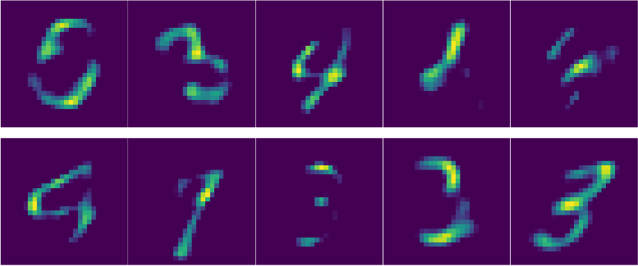
We first randomly select some empirical examples to visually show performance comparison in Figure 3. In these examples, observations are perturbed with some Gaussian random noise with variance $0.3$ and we use $\ell_{\infty}$ LP as our algorithm to invert the network. From the figures, we could see that our method could almost perfectly denoise and reconstruct the input image, while gradient descent impairs the completeness of the original images to some extent.

We also compare the distribution of relative recovery error with respect to different input noise levels, as ploted in Figure 1(c)(d). From the figures, we observe that for this real network, our proposals still successfully recover the ground truth with good accuracy most of the time, while gradient descent usually gets stuck in local minimum. This explains why it produces defective image reconstructions as shown in 3.

Finally, we presented some sensing results when we mask part of the observations using PGD with our inverting procedure. As shown in Figure 4, our algorithm always show reliable recovery while gradient descent sometimes fails to output reasonable result. More experiments are presented in the Appendix.

References

- [1] Zeyuan Allen-Zhu, Rati Gelashvili, and Ilya Razenshteyn. Restricted isometry property for general p-norms. IEEE Transactions on Information Theory, 62(10):5839–5854, 2016.
- [2] Benjamin Aubin, Bruno Loureiro, Antoine Maillard, Florent Krzakala, and Lenka Zdeborová. The spiked matrix model with generative priors. arXiv preprint arXiv:1905.12385, 2019.
- [3] Radu Berinde, Anna C Gilbert, Piotr Indyk, Howard Karloff, and Martin J Strauss. Combining geometry and combinatorics: A unified approach to sparse signal recovery. In Communication, Control, and Computing, 2008 46th Annual Allerton Conference on, pages 798–805. IEEE, 2008.
- [4] Ashish Bora, Ajil Jalal, Eric Price, and Alexandros G Dimakis. Compressed sensing using generative models. arXiv preprint arXiv:1703.03208, 2017.
- [5] Manik Dhar, Aditya Grover, and Stefano Ermon. Modeling sparse deviations for compressed sensing using generative models. arXiv preprint arXiv:1807.01442, 2018.
- [6] Alyson K Fletcher and Sundeep Rangan. Inference in deep networks in high dimensions. arXiv preprint arXiv:1706.06549, 2017.
- [7] Gene H Golub and Charles F Van Loan. Matrix computations, volume 3. JHU Press, 2012.
- [8] Ian Goodfellow, Jean Pouget-Abadie, Mehdi Mirza, Bing Xu, David Warde-Farley, Sherjil Ozair, Aaron Courville, and Yoshua Bengio. Generative adversarial nets. In Advances in neural information processing systems, pages 2672–2680, 2014.
- [9] Aditya Grover and Stefano Ermon. Uncertainty autoencoders: Learning compressed representations via variational information maximization. arXiv preprint arXiv:1812.10539, 2018.
- [10] Sidharth Gupta, Konik Kothari, Maarten V de Hoop, and Ivan Dokmanić. Deep mesh projectors for inverse problems. arXiv preprint arXiv:1805.11718, 2018.
- [11] Paul Hand, Oscar Leong, and Vlad Voroninski. Phase retrieval under a generative prior. In Advances in Neural Information Processing Systems, pages 9154–9164, 2018.
- [12] Paul Hand and Vladislav Voroninski. Global guarantees for enforcing deep generative priors by empirical risk. arXiv preprint arXiv:1705.07576, 2017.
- [13] Reinhard Heckel and Paul Hand. Deep decoder: Concise image representations from untrained non-convolutional networks. arXiv preprint arXiv:1810.03982, 2018.
- [14] Reinhard Heckel, Wen Huang, Paul Hand, and Vladislav Voroninski. Deep denoising: Rate-optimal recovery of structured signals with a deep prior. arXiv preprint arXiv:1805.08855, 2018.
- [15] Wen Huang, Paul Hand, Reinhard Heckel, and Vladislav Voroninski. A provably convergent scheme for compressive sensing under random generative priors. arXiv preprint arXiv:1812.04176, 2018.
- [16] Piotr Indyk and Ilya Razenshteyn. On model-based rip-1 matrices. In International Colloquium on Automata, Languages, and Programming, pages 564–575. Springer, 2013.
- [17] Morteza Mardani, Qingyun Sun, Shreyas Vasawanala, Vardan Papyan, Hatef Monajemi, John Pauly, and David Donoho. Neural proximal gradient descent for compressive imaging. arXiv preprint arXiv:1806.03963, 2018.
- [18] Dustin G Mixon and Soledad Villar. Sunlayer: Stable denoising with generative networks. arXiv preprint arXiv:1803.09319, 2018.
- [19] Mergen Nachin. Lower bounds on the column sparsity of sparse recovery matrices. UAP: MIT Undergraduate Thesis, 2010.
- [20] Parthe Pandit, Mojtaba Sahraee, Sundeep Rangan, and Alyson K Fletcher. Asymptotics of map inference in deep networks. arXiv preprint arXiv:1903.01293, 2019.
- [21] Yaniv Romano, Michael Elad, and Peyman Milanfar. The little engine that could: Regularization by denoising (red). SIAM Journal on Imaging Sciences, 10(4):1804–1844, 2017.
- [22] Mark Rudelson and Roman Vershynin. Smallest singular value of a random rectangular matrix. Communications on Pure and Applied Mathematics: A Journal Issued by the Courant Institute of Mathematical Sciences 62.12, pages 1707–1739, 2009.
- [23] Viraj Shah and Chinmay Hegde. Solving linear inverse problems using gan priors: An algorithm with provable guarantees. arXiv preprint arXiv:1802.08406, 2018.
- [24] Subarna Tripathi, Zachary C Lipton, and Truong Q Nguyen. Correction by projection: Denoising images with generative adversarial networks. arXiv preprint arXiv:1803.04477, 2018.
Appendix A Methodology Details
In this section we present the detailed steps for our proposed methods.
A.1 LP Relaxation
We formally present the relaxed version based on (8):