Cusp transitivity in hyperbolic 3-manifolds
Abstract
Let be a cusped finite-volume hyperbolic three-manifold with isometry group . Then induces a -transitive action by permutation on the cusps of for some integer . Generically is trivial and , but does occur in special cases. We show examples with . An interesting question concerns the possible number of cusps for a fixed . Our main result provides an answer for by constructing a family of manifolds having no upper bound on the number of cusps.
1 Introduction
An action of a group on a set is called -transitive if, for every choice of distinct elements and every choice of distinct targets , there is an element such that . The term transitive means 1-transitive; actions with are multiply transitive. The number of elements in is the degree. Transitive actions are common (for example, every group acts transitively on itself by left multiplication), while multiply-transitive actions are relatively rare. The theory is well developed; see [4].
It is obvious that the isometry group of a complete finite-volume hyperbolic three-manifold induces a permutation action on the set of cusps. In this paper we call such a manifold k-transitive if the induced action is -transitive. Note that this definition is of the ‘inclusive hierarchy’ type. For instance, a 3-transitive manifold is automatically 2-transitive, and possibly 4-transitive as well.
Kojima [8] shows by construction that every finite group occurs as the isometry group of some closed hyperbolic 3-manifold. At one stage, the construction involves a cusped manifold, with cusps labeled by the elements of . The induced permutation action on the cusp set amounts to left-multiplication of the labels by elements of . Since this action is transitive, the manifold at this stage is 1-transitive by our definition, and we see that 1-transitive manifolds are plentiful and can have any number of cusps. But the action is also free, which implies that it is never 2-transitive. Hence one may begin to wonder, for , how common and how challenging to construct are the -transitive manifolds?
In Section 2 we give some examples of 1-, 2- and 4-transitive manifolds, all constructed as complements of hyperbolic links in . In Section 3 we show a construction that leads to our main result:
Theorem 1
For the class of 2-transitive manifolds, there is no upper bound on the number of cusps.
In Section 4 we summarize known results and mention some open questions.
2 Examples with
All the manifolds in this section are link complements in . The constructions are easy, so we give only brief descriptions. The key idea is that, since the geometric structure of a hyperbolic link complement is unique, symmetries of the link are always realized by isometries of the complement. Where no outside reference is given, hyperbolicity has been verified using SnapPea [14].
2.1 A chain construction
Consider a cycle of unknotted loops, , linked sequentially, and having half-twists, , as in Figure 1. The chain itself, viewed as a single loop, must be unknotted. There is an obvious 1-transitive cyclic action on the link components.
Two sub-families of such chains appear as examples in Thurston’s notes, and the complete family is analyzed by Neumann and Reid [9]. They show that for the link is hyperbolic for every value of , and for the link is hyperbolic for all but values of , the exceptions being the cases with the least overall twisting.
2.2 A braid construction
Suppose is a pseudo-Anosov braid on strands for which the associated permutation is cyclic of order . Then the braid induces the trivial permutation on the strands, and the closure of is thus a link having components. Again, there is an obvious 1-transitive cyclic action. An example is shown in Figure 2.
The closed braid might fail to be hyperbolic. In particular, since a braid is closed by performing a Dehn filling on the braid axis, it might happen that the meridian is too short to allow a hyperbolic filling. In this case, the longer braid will have meridian times as long, and thus, by the ‘ theorem’ of Gromov and Thurston [3], the closed braid will be hyperbolic for sufficiently large . (It seems likely that the th power of is already enough to guarantee a meridian longer than , but there may be exceptions to this.)
2.3 Two cubical constructions
Consider the four planes in given by , with . These planes are perpendicular to the four diagonals of the cube with vertices . Intersecting these planes with the unit sphere gives four great circles intersecting at twelve points. By resolving each intersection to an over- or under-crossing, in alternating fashion, a hyperbolic link is obtained. A planar diagram is shown in Figure 3 (Left).
The group of orientation-preserving symmetries of the cube carries over naturally to the link components, and it is an easy exercise to check that this action is 4-transitive. This link can also be obtained by the braid construction given above, but the 4-transitivity is not so obvious.
An analogous construction, where the cube is replaced by an icosahedron, yields a 2-transitive manifold having 6 cusps.
The second cubical construction builds a 12-component link by following the structure of the edges of a cube, as shown in Figure 3. The complement is hyperbolic and 1-transitive. In contrast to the chain and braid examples shown earlier, the action is non-cyclic.
3 A family of 2-transitive manifolds
In this section we construct an infinite family of 2-transitive manifolds for which the number of cusps increases without bound. The construction builds on a family of regular maps described by Biggs [2] and further studied by James and Jones [7].
Here is an overview of the construction. Let be a surface carrying one of the regular maps of Biggs. There is a natural 2-transitive action on the faces of this map by its automorphism group. The product is formed, and within this non-hyperbolic manifold a system of simple closed curves is specified. The curves are carefully designed to maintain the original 2-transitive symmetry. The complement of this link is the desired manifold . Finally, to verify that is hyperbolic, it is viewed as a punctured-surface bundle over with pseudo-Anosov monodromy.
We now describe the construction in more detail. Let be a prime power greater than 3, and let F be the finite field of order . Biggs uses the arithmetic of F to construct orientable regular maps (tessellations) on a closed surface. Such a map has faces, each face a -gon. The genus of the surface is given by
The faces admit a natural labeling by the elements of F, and the automorphism group of the map is exactly the natural action of the affine group on the face labels. The 2-transitivity of this action is an easy exercise. The significance of this, combinatorially, is that each face of the map shares an edge with each of the remaining faces.
We take to be the orientable surface carrying this regular map, endowed with the natural constant-curvature metric (see [5]). The case is used in the illustrations; the surface is a square torus tiled by five square faces.
The construction continues inside a preliminary three-manifold , where is the unit interval. For each face of , arcs are specified in as follows. First, let be the center point of , and let be the circle of radius and circumference in centered at . Let the vertices of be denoted sequentially around the perimeter, for . Let be the point of intersection of and the radial segment extending from to . Now is a cylinder surrounding the fiber in . The desired arcs are defined to be the helical segments of slope lying on , each extending from the image of in to the image of in (indices modulo ). Figure 4 illustrates this step.
Next, is formed by identifying the two boundary components of by equality in the first factor; hence is the product . By this identification the cylinder becomes a torus, and the segments join end-to-end yielding a closed curve, namely, a torus knot.
Finally, to obtain the desired link, we adjust the size of circle as follows. A face of has two characteristic radii: , the distance from center to an edge midpoint, and , the distance from to a vertex. By requiring the radius to satisfy , each copy of lies partly on its own face and partly on the neighboring faces. Hence each strand of the corresponding torus knot extends radially outward just far enough to link with a strand of the neighboring knot. Manifold is now defined to be the complement in of this link.
In , each original cross section (for ) is now a punctured surface, since the points of intersection with the strands of the link are now missing. For convenience in the subsequent analysis, we specify the cross section at level with respect to the original factor as the ‘base surface’ and observe that is the mapping torus of a point-pushing homeomorphism of this surface. A diagram for is shown in Figure 5.
A homeomorphism is pseudo-Anosov if there exists a pair of transverse singular foliations, and , invariant under , and an associated constant , the dilatation. The surface is stretched and compressed along the two foliations by factors of and , respectively. By a result of Thurston [12], the mapping torus of a pseudo-Anosov homeomorphism is hyperbolic.
Figure 6 shows an approximation of the foliation for . Singularities occur at the vertices and face-centers of the underlying map; these points are fixed by . A train track for , as discussed by Bestvina and Handel [1], is also shown. The structure of the track is equivariant with respect to the symmetries of the surface. The complement of the track consists of once-punctured monogons and cusp-cornered polygons. The track captures in a discrete way the overall structure of the foliation, and is mapped, with appropriate stretching, onto itself by (modulo some adjustment homotopic to the identity). Details for the theory of train tracks are given by Penner and Harer [10].
We turn next to the calculation of and the weights associated to branches of the track. A few different approaches to this problem are possible. The underlying symmetry allows some simplifications to be made.
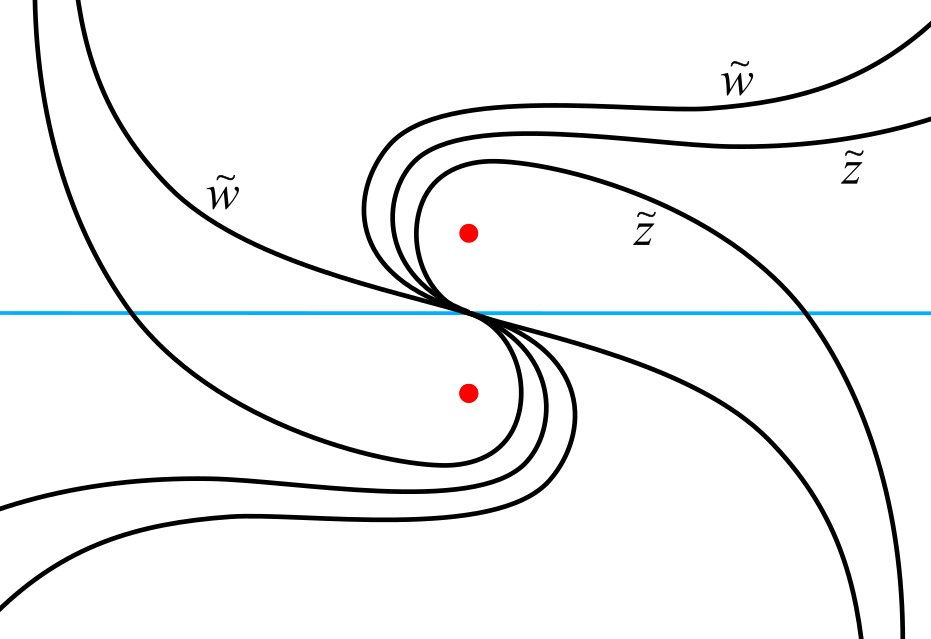
In Figure 7 the points labeled through are punctures, while is a fixed point of . Each branch of the track is assigned a positive weight. The weights determine a crossing measure for transverse arcs. Two branches in the diagram are assigned weights and ; the weights for all other branches are determined by symmetry and by the summation rule where branches merge. Thus each semicircular branch that half-surrounds a puncture has weight and each very short branch found between a pair of nearest-neighbor punctures has weight .
Arc crosses 17 branches and has total crossing measure . Its image under is arc , which has crossing measure . One may view this as compression by in the transverse () direction, resulting in the full weight being forced onto a portion of track that previously carried just . Since the contraction factor for the compression is , one may attribute the increased ‘density’ to a scaling by ; hence
| (1) |
Similarly, arc has measure , while its image, arc , has measure , and we obtain
| (2) |
With these two equations, we have enough constraints to determine the unknowns. Since weights are determined only up to a scale factor, we can set and solve, first obtaining , and then
and
This quick solution may seem a bit ad hoc; for a more systematic view of things let us divide both sides of equation (1) by 2 and then subtract equation (2) to produce
| (3) |
Equations (2) and (3) together now form a linear system
and we see how the weights constitute an eigenvector for eigenvalue .
A related (and the most standard) approach is based on viewing the train track as an embedded graph and analyzing the self-map induced on it by . Every branch is assigned a numerical value; these correspond to a tangential measure, and may be interpreted simply as edge lengths. The map stretches each edge onto some sequence of edges; this data is encoded by an incidence matrix. The stretched length is then some particular sum of original edge lengths, and one wishes to attribute all the stretching to a single scale factor. This, of course, is again an eigenvalue problem.
The full incidence matrix of a train track for is rather large, but two easy simplifications make the problem tractable. First we modify the track as shown in Figure 8, so there are just two classes of branches. These are labeled and . Then we replace the incidence matrix by a two-by-two matrix that imposes the same constraints on edge lengths that are implicit in the incidence matrix. Using the diagrams in Figures 5 through 8 it is rather straightforward to trace out the image of a edge: it is stretched onto a sequence of edges of type . Similarly, a edge is mapped onto . Hence we have
The matrix for this linear system is just the transpose of the one that occurred earlier, so the eigenvalues are unchanged. The weights and for the tangential measure are the reciprocals (up to a scale factor) of those obtained earlier for the transverse measure. An overview of these concepts, placing them in the larger context of Thurston’s work, can be found in the Epilogue of [10].
Yet another approach to analyzing has been generously pointed out by an anonymous referee. Due to the large symmetry group , the associated quotient space of is quite simple. A fundamental domain consists of two neighboring triangles in the barycentric subdivision of a face, and the induced edge identifications yield a topological sphere with three cone points, something like a triangular pillow or a turnover pastry. The punctures all get identified to a single point of the quotient; removing this point, along with the three cone points, produces a four-punctured sphere. This surface has a natural metric coming from its two-covering by a flat torus via the classical elliptic involution, with the four fixed points corresponding to the punctures. The image of in this reduced setting can be analyzed explicitly using Dehn twists, and its lift to the torus is a genuine Anosov transformation having scale factors . Details for these steps can be found in [1], [13], and the primer [6] by Farb and Margalit.
The details used in the above approaches (specifically, the diagrams in Figures 7 and 8, and the nature of the quotient space) do not depend on the faces being squares. Thus the computations work out as shown not just for , but for every prime-power value of . Hence the same dilatation occurs in every case.
4 Further questions
The constructions shown in Section 2, along with Kojima’s method, suggest that 1-transitive manifolds may allow for quite a diversity of structures. It would be interesting to find a more systematic understanding of the big picture.
For , more examples can be produced by easy variations of the above construction based on the Biggs surfaces. Are there other 2-transitive manifolds having substantially different structure? Is every 2-transitive group action realized by some 2-transitive manifold?
There are lots of 3-transitive manifolds having just three cusps, but this is not too surprising since a 3-transitive action on a set of three objects is not really very exotic. In particular, the three-component chain links described earlier all have obvious 3-transitive symmetry, and all but two of them are hyperbolic. The famous Borromean rings are another example. For more than three cusps, the situation appears much harder. The author is aware of one 3-transitive manifold with six cusps, and another with eight, but no others.
For , our only known example is the manifold described in Section 2, and easy variations of it, all having four cusps.
In the original version of this paper we stated two conjectures: that there is a largest for which -transitive manifolds exist, and that for each there is an upper bound on the possible number of cusps. Both have since been proven, and sharp bounds provided, by Ratcliffe and Tschantz [11].
References
- [1] Mladen Bestvina and Michael Handel, Train-tracks for surface homeomorphisms, Topology 34 (1995), no. 1, 109–140.
- [2] Norman L. Biggs, Automorphisms of imbedded graphs, Journal of Combinatorial Theory, Series B 11 (1971), 132–138.
- [3] Steven A Bleiler and Craig D Hodgson, Spherical space forms and dehn filling, Topology 35 (1996), no. 3, 809–833.
- [4] John D. Dixon and Brian Mortimer, Permutation groups, Graduate Texts in Mathematics, vol. 163, Springer-Verlag, New York, 1996. MR 1409812 (98m:20003)
- [5] Allan L Edmonds, John H Ewing, and Ravi S Kulkarni, Regular tessellations of surfaces and (p, q, 2)-triangle groups, Annals of Mathematics (1982), 113–132.
- [6] Benson Farb and Dan Margalit, A primer on mapping class groups (pms-49), Princeton University Press, 2011.
- [7] Lynne D. James and Gareth A. Jones, Regular orientable imbeddings of complete graphs, Journal of Combinatorial Theory, Series B 39 (1985), 353–367.
- [8] Sadayoshi Kojima, Isometry transformations of hyperbolic 3-manifolds, Topology and its Applications 29 (1988), no. 3, 297–307.
- [9] Walter D Neumann and Alan W Reid, Arithmetic of hyperbolic manifolds, Topology 90 (1992), 273–310.
- [10] R. C. Penner and J. L. Harer, Combinatorics of train tracks, Annals of Mathematics Studies, vol. 125, Princeton University Press, Princeton, NJ, 1992. MR 1144770 (94b:57018)
- [11] John G Ratcliffe and Steven T Tschantz, Cusp transitivity in hyperbolic 3-manifolds, arXiv preprint arXiv:1912.04192 (2019).
- [12] William P Thurston, Three-dimensional manifolds, Kleinian groups and hyperbolic geometry, Bull. Amer. Math. Soc. (N.S.) 6 (1982), no. 3, 357–381. MR 648524 (83h:57019)
- [13] , On the geometry and dynamics of diffeomorphisms of surfaces, Bulletin (new series) of the American Mathematical Society 19 (1988), no. 2, 417–431.
- [14] Jeff Weeks, SnapPea, 1999.
Department of Mathematical Sciences, Central Connecticut State University, New Britain, Connecticut 06050, USA
vogelerrov@ccsu.edu