MPEG-2 Prediction Residue Analysis

The use of an intra-coding mode during the second compression yields $\hat{\mathbf{Y}}_{n}=0$, such that $\mathbf{W}_{n}=\mathbf{Y}_{n}$. Hence, from (8), the variance of the resulting prediction residue can be expressed as

$$\text{Var}\left(\mathbf{W}_{n}\right)=\begin{cases}\text{Var}\left(\mathbf{X}_{n}\right)+\text{Var}\left(\mathbf{E}_{n}^{\text{I}_{1}}\right),&\text{if }n\in\mathsf{I}_{1}\\ \text{Var}\left(\mathbf{X}_{n}\right)+\text{Var}\left(\mathbf{E}_{n}^{\text{P}_{1}}\right),&\text{if }n\in\mathsf{P}_{1}\end{cases},$$

(9)

where we assume that the quantization errors $\mathbf{E}_{n}^{\text{I}_{1}}$ and $\mathbf{E}_{n}^{\text{P}_{1}}$ have negligible correlation with the source signal $\mathbf{X}_{n}$. This assumption typically holds whenever the probability density function (pdf) of the source signal is smooth and its variance is much larger than the employed quantization step sizes, which is generally the case in practice. By inserting the relationship (9) in (7), the strength of the VPF can be evaluated in this case by means of

$$\text{Var}\left(\mathbf{E}_{n}^{\text{I}_{1}}\right)-\text{Var}\left(\mathbf{E}_{n}^{\text{P}_{1}}\right).$$

The variance of both quantization errors can be analytically described conforming to the model discussed in Section 2, as follows:

1. 1.

   $\text{Var}\left(\mathbf{E}_{n}^{\text{I}_{1}}\right)$: given the definition of $\mathbf{E}_{n}^{\text{I}_{1}}$, its variance is proportional (except for a constant normalization factor) to the distortion between the reconstructed samples $\mathbf{X}_{n}^{\prime}$ and their source $\mathbf{X}_{n}$ when the SSD measure is considered, thus having

   $$\text{Var}\left(\mathbf{E}_{n}^{\text{I}_{1}}\right)\propto D\left(\mathbf{X}_{n},\mathbf{X}_{n}^{\prime}\right)\triangleq\|\mathbf{X}_{n}-\mathbf{X}_{n}^{\prime}\|_{2}^{2}.$$

   Since the DCT adopted in MPEG-2 has orthogonal basis (discarding rounding effects in the DCT calculation), the above distortion can be directly computed in the transformed domain as

   $$D\left(\mathbf{X}_{n},\mathbf{X}_{n}^{\prime}\right)=\sum_{i=0}^{7}\sum_{j=0}^{7}D_{X}(i,j),$$

   where $D_{X}(i,j)$ represents the distortion of the $(i,j)$-th DCT coefficient. In line with the quantization model introduced in Section 2, the values of $D_{X}(i,j)$ (except for the DC coefficient) are given by

   	$\displaystyle D_{X}(i,j)=$	$\displaystyle\int_{-\frac{\alpha_{\text{I}}}{2}\Delta_{1}^{\text{I}}}^{\frac{\alpha_{\text{I}}}{2}\Delta_{1}^{\text{I}}}x^{2}f_{X}(x)~dx$
   		$\displaystyle+2\sum_{k=1}^{\infty}\int_{(k-1+\frac{\alpha_{\text{I}}}{2})\Delta_{1}^{\text{I}}}^{(k+\frac{\alpha_{\text{I}}}{2})\Delta_{1}^{\text{I}}}\left(x-\left\lfloor k\Delta_{1}^{\text{I}}\right\rfloor\right)^{2}f_{X}(x)~dx,$		(10)

   where $f_{X}(x)$ denotes the pdf of the corresponding AC coefficient which, as discussed at the end of Section 2, can be modeled as a Laplacian distribution with mean $\mu_{X}$ and variance $\sigma_{X}^{2}$.

   From the above equation we observe that for a fixed value of $\sigma_{X}^{2}$, the evolution of $\text{Var}\left(\mathbf{E}_{n}^{\text{I}_{1}}\right)$ mostly depends on the deadzone width (configured through the parameter $\alpha_{\text{I}}$) and on the quantization step $\Delta_{1}^{\text{I}}$ (controlled by the quantization parameter $\text{Q}_{1}$ as in (2)). More specifically, we can state that larger values of $\alpha_{\text{I}}$ (or, equivalently, wider deadzones) yield larger values of $\text{Var}\left(\mathbf{E}_{n}^{\text{I}_{1}}\right)$, which also increases with $\text{Q}_{1}$, since larger values of $\text{Q}_{1}$ produce coarser quantization steps $\Delta_{1}^{\text{I}}$.

2. 2.

   $\text{Var}\left(\mathbf{E}_{n}^{\text{P}_{1}}\right)$: the variance of the quantization error $\mathbf{E}_{n}^{\text{P}_{1}}$ satisfies the following relation

   	$\displaystyle\text{Var}\left(\mathbf{E}_{n}^{\text{P}_{1}}\right)$	$\displaystyle\propto\text{p}(\text{I-MB})D(\mathbf{X}_{n},\mathbf{X}_{n}^{\prime})+\text{p}(\text{P-MB})D(\mathbf{U}_{n},\mathbf{U}_{n}^{\prime})$
   		$\displaystyle\quad+\text{p}(\text{S-MB})D(\mathbf{X}_{n},\mathbf{X}_{n\!-\!1}^{\prime}),$

   where $\text{p}(\text{c})$ denotes the probability of using the coding mode $\text{c}\!\in\!\mathcal{C}$ per frame. Regarding the distortion terms, both $D(\mathbf{X}_{n},\mathbf{X}_{n}^{\prime})$ and $D(\mathbf{X}_{n},\mathbf{X}_{n-1}^{\prime})$ can be computed as in the previous case through (10),²² 2 Note that for $D(\mathbf{X}_{n},\mathbf{X}_{n\!-\!1}^{\prime})$, only an approximation would be obtained through (10), but still valid in practice since $\mathbf{X}_{n}\approx\mathbf{X}_{n\!-\!1}$ for S-MBs. whereas $D(\mathbf{U}_{n},\mathbf{U}_{n}^{\prime})$ can be obtained by accumulating the distortion of each $(i,j)$-th DCT coefficient, i.e., $D(\mathbf{U}_{n},\mathbf{U}_{n}^{\prime})=\sum_{i=0}^{7}\sum_{j=0}^{7}D_{U}(i,j)$, where $D_{U}(i,j)$ is given by

   	$\displaystyle D_{U}(i,j)=$	$\displaystyle\int_{-\frac{\alpha_{\text{P}}}{2}\Delta_{1}^{\text{P}}}^{\frac{\alpha_{\text{P}}}{2}\Delta_{1}^{\text{P}}}u^{2}f_{U}(u)~du$
   		$\displaystyle+2\sum_{k=1}^{\infty}\int_{(k-1+\frac{\alpha_{\text{P}}}{2})\Delta_{1}^{\text{P}}}^{(k+\frac{\alpha_{\text{P}}}{2})\Delta_{1}^{\text{P}}}\left(u\!-\!\left\lfloor k\Delta_{1}^{\text{P}}+\frac{\Delta_{1}^{\text{P}}}{2}\right\rfloor\right)^{2}f_{U}(u)~du.$

   In the above equation, $f_{U}(u)$ denotes the pdf of the $(i,j)$-th DCT coefficient which can be modeled as a Laplacian distribution with zero mean and variance $\sigma_{U}^{2}$ [7].

   Similarly to the previous case, $\text{Var}\left(\mathbf{E}_{n}^{\text{P}_{1}}\right)$ also monotonically increases with $\text{Q}_{1}$, although now the effect of the deadzone width is a function of both parameters $\alpha_{\text{I}}$ and $\alpha_{\text{P}}$. The influence of each deadzone width will depend on the type of scene to be encoded, since its content will finally rule the probability of using each type of MB. For instance, in static scenes, it is common to have $\text{p}(\text{S-MB})\gg\text{p}(\text{P-MB})+\text{p}(\text{I-MB})$, so $\text{Var}\left(\mathbf{E}_{n}^{\text{P}_{1}}\right)$ will increase with $\text{Q}_{1}$ and $\alpha_{\text{I}}$, and will not be excessively affected by $\alpha_{\text{P}}$, whereas in dynamic scenes, where almost all the coded MBs have a non-zero motion vector with $\mathbf{U}_{n}^{\prime}\neq 0$, such that $\text{p}(\text{P-MB})\gg\text{p}(\text{S-MB})+\text{p}(\text{I-MB})$, the evolution of $\text{Var}\left(\mathbf{E}_{n}^{\text{P}_{1}}\right)$ will be mostly governed by $\alpha_{\text{P}}$ instead of $\alpha_{\text{I}}$.

The above findings can be checked in Fig. 2, where the evolution of $\text{Var}\left(\mathbf{E}_{n}^{\text{I}_{1}}\right)$ and $\text{Var}\left(\mathbf{E}_{n}^{\text{P}_{1}}\right)$ for the $(1,0)$-th DCT coefficient is shown for two videos gathered from [8]: the static video akiyo in Fig. 2(a), and the dynamic video mobile in Fig. 2(b). In the static case reported in Fig. 2(a), the evolution of $\text{Var}\left(\mathbf{E}_{n}^{\text{P}_{1}}\right)$ at $(1,0)$ mostly depends on $\alpha_{\text{I}}$ due to the role of the S-MBs that fundamentally make reference to MBs from the previously encoded I-frame, thus yielding a quantization error $\mathbf{E}_{n}^{\text{P}_{1}}$ very similar to $\mathbf{E}_{n}^{\text{I}_{1}}$. On the other hand, when dealing with dynamic scenes as in Fig. 2(b), $\text{Var}\left(\mathbf{E}_{n}^{\text{P}_{1}}\right)$ at $(1,0)$ does not depend on $\alpha_{\text{I}}$, instead it is governed by $\alpha_{\text{P}}$ given that the curves for different values of $\alpha_{\text{I}}$ are close to each other.

From the above analysis, it follows that for static video sequences, the difference $\text{Var}\left(\mathbf{E}_{n}^{\text{I}_{1}}\right)-\text{Var}\left(\mathbf{E}_{n}^{\text{P}_{1}}\right)$ is small and so $\text{Var}\left(\mathbf{W}_{n}\right)|_{n\in\mathsf{I}_{1}}\approx\text{Var}\left(\mathbf{W}_{n}\right)|_{n\in\mathsf{P}_{1}}$, while for dynamic videos it is harder to define a similar relation. In fact, the varying nature of the prediction residue with dynamic videos complicates the modeling (i.e., at least a motion estimation of the scene would be needed), thus we leave its study for a future work. In constrast, the nearly constant behavior of $\text{Var}\left(\mathbf{W}_{n}\right)$ under the intra prediction (independently of the type of frame used in the first compression), implies that for low-motion videos, the presence of the VPF is ultimately guided by the behavior of $\text{Var}\left(\mathbf{W}_{n}\right)$ under the inter prediction, which we analyze in the following Section 3.2.

Prior to address the evolution of the residue under the inter-prediction setting, we introduce the proposed semi-analytic model to predict the behavior of $\text{Var}\left(\mathbf{E}_{n}^{\text{I}_{1}}\right)$ and $\text{Var}\left(\mathbf{E}_{n}^{\text{P}_{1}}\right)$ for static video sequences. To that end, we use a first-order autoregressive process $x_{n}$ for modeling the temporal dependencies of the source signal $\mathbf{X}_{n}$. Troughout the paper we will consider three distinct time indices: $n-2$, $n-1$, and $n$, and we will correspondingly define three stochastic processes: $x_{n-2}$, $x_{n-1}$, and $x_{n}$. Thus, assuming the stochastic process $x_{n-2}$ follows a Laplacian distribution with zero mean and variance $\sigma_{X}^{2}=2500$, we generate the remaining stochastic processes as $x_{n-1}=\rho x_{n-2}+r_{n-1}$ and $x_{n}=\rho x_{n-1}+r_{n}$, where we take $\rho=0.99$ to simulate the high temporal correlation between adjacent frames in low-motion videos and we define the residue signal $r_{n}$ as a zero-mean Gaussian process with variance $\sigma_{R}^{2}=10$. On the other hand, the inter-prediction process is also characterized through a first-order autoregressive process, such that $\hat{\mathbf{X}}_{n}=\mathbf{X}_{n-1}^{\prime}(\mathbf{m})$ is modeled through the stochastic process $\hat{x}_{n}=\rho_{\text{P}}x_{n-1}^{\prime}+\nu_{n}$, where we take $\rho_{\text{P}}=0.88$ to simulate the effect of a non-perfect motion estimation and we make use of a zero-mean Gaussian process $\nu_{n}$ with variance $\sigma_{\nu}=1$ to mimic the effect of the motion compensation through $\mathbf{m}$. During the first compression, we assume that at time index $n-2$ there is always an I-frame, then at $n-1$ a P-frame, and finally at $n$, it will depend on the case under study, i.e., $n\in\mathsf{I}_{1}$ or $n\in\mathsf{P}_{1}$. For the second compression, an I-frame is also assumed at $n-2$, and a P-frame at $n-1$.

Now, from the definition of $\mathbf{E}_{n}^{\text{I}_{1}}$, we generate the samples of the corresponding synthetic signal as $e_{n}^{\text{I}_{1}}=x_{n}^{\prime}-x_{n}$, where all the samples from $x_{n}$ are first quantized as in (4) for I-MBs (using $\Delta_{1}^{\text{I}}$ and $\alpha_{\text{I}}$) and then are accordingly reconstructed through (5) to obtain $x_{n}^{\prime}$. On the other hand, the synthetic signal for $\mathbf{E}_{n}^{\text{P}_{1}}$, must consider the different coding modes from $\mathcal{C}$ that can be used when a P-frame is encoded. Without loss of generality, we assume that the number of I-MBs in static videos is negligible, such that $\text{p}(\text{I-MB})\rightarrow 0$, which is commonly the case in practice. Regarding the modeling of P-MBs, we assume that $\text{p}(\text{P-MB})$ decreases as $\text{Q}_{1}$ grows (which is the expected behavior in low-motion videos), so we use $\text{p}(\text{P-MB})=p_{1}$ with $p_{1}\triangleq 0.15+0.7e^{-9\frac{\text{Q}_{1}}{\text{Q}_{\max}}}$, where $\text{Q}_{\max}=31$ denotes the maximum allowed quantization parameter. Accordingly, we set $\text{p}(\text{S-MB})=1-p_{1}$ and we finally compute the synthetic signal for $\mathbf{E}_{n}^{\text{P}_{1}}$ as

$$e_{n}^{\text{P}_{1}}=\begin{cases}u_{n}^{\prime}-u_{n},&\text{if }\text{c}=\text{P-MB}\\ x_{n-1}^{\prime}-x_{n},&\text{otherwise}\\ \end{cases},$$

where $u_{n}=x_{n}-\hat{x}_{n}$ and $u_{n}^{\prime}$ is obtained by first quantizing $u_{n}$ as in the second case of (4) and then reconstructing its samples through (5) (in both cases, using $\Delta_{1}^{\text{P}}$ and $\alpha_{\text{P}}$). Finally, to obtain $x_{n-1}^{\prime}$, the whole encoding process of a P-frame must be applied, so with probability $1-p_{1}$, the samples of $x_{n-1}^{\prime}$ stem from the use of the first case in (4)-(5) over the samples of $x_{n-1}$ (using $\Delta_{1}^{\text{I}}$ and $\alpha_{\text{I}}$). On the other hand, with probability $p_{1}$, the corresponding signal $u_{n-1}=x_{n-1}-\hat{x}_{n-1}$ must be computed, where $\hat{x}_{n-1}$ is given through $\hat{x}_{n-1}=\rho_{\text{P}}x_{n-2}^{\prime}+\nu_{n-1}$ with $x_{n-2}^{\prime}$ being the result of reconstructing the whole signal $x_{n-2}$ as the encoding of an I-frame. Once $u_{n-1}$ is computed, then the second case in (4) and (5) must be applied to generate $u_{n-1}^{\prime}$, which finally allows the calculation of $x_{n-1}^{\prime}=u_{n-1}^{\prime}+\hat{x}_{n-1}$.

The result of using this semi-analytic approach to predict the behavior of $\text{Var}\left(\mathbf{E}_{n}^{\text{I}_{1}}\right)$ and $\text{Var}\left(\mathbf{E}_{n}^{\text{P}_{1}}\right)$ in the DCT domain at $(1,0)$ for static video sequences is illustrated in Fig. 2(c), which closely resembles its empirical counterpart in Fig. 2(a).

In this case, $\hat{\mathbf{Y}}_{n}$ is the result of an inter prediction, i.e., $\hat{\mathbf{Y}}_{n}=\mathbf{Y}_{n-1}^{\prime}(\mathbf{m})$. Assuming that the estimated motion scene through $\mathbf{m}$ coincides in the two consecutive compressions (which is reasonable in practice, provided that the content of the scene remains unchanged across both compressions), $\hat{\mathbf{Y}}_{n}$ can be expressed as

	$\displaystyle\hat{\mathbf{Y}}_{n}$	$\displaystyle=\mathbf{Y}_{n-1}(\mathbf{m})+\mathbf{E}_{n-1}^{\text{P}_{2}}$
		$\displaystyle=\mathbf{X}_{n-1}(\mathbf{m})+\mathbf{E}_{n-1}^{\text{P}_{1}}+\mathbf{E}_{n-1}^{\text{P}_{2}},$		(11)

where $\mathbf{E}_{n-1}^{\text{P}_{1}}\triangleq\mathbf{U}_{n-1}^{\prime}(\mathbf{m})-\mathbf{U}_{n-1}(\mathbf{m})$ and $\mathbf{E}_{n-1}^{\text{P}_{2}}\triangleq\mathbf{W}_{n-1}^{\prime}(\mathbf{m})-\mathbf{W}_{n-1}(\mathbf{m})$ represent the quantization errors that result from the first and second compression, respectively. Using (8) and (11) in the definition of $\mathbf{W}_{n}$, we obtain

$$\mathbf{W}_{n}=\mathbf{R}_{n}+\mathbf{E}_{n},\quad\text{with}\quad\mathbf{E}_{n}=\begin{cases}\mathbf{E}_{n}^{\text{I}_{1}}-\mathbf{E}_{n-1}^{\text{P}_{1}}-\mathbf{E}_{n-1}^{\text{P}_{2}},&\text{if }n\in\mathsf{I}_{1}\\ \mathbf{E}_{n}^{\text{P}_{1}}-\mathbf{E}_{n-1}^{\text{P}_{1}}-\mathbf{E}_{n-1}^{\text{P}_{2}},&\text{if }n\in\mathsf{P}_{1}\end{cases},$$

where $\mathbf{R}_{n}\triangleq\mathbf{X}_{n}-\mathbf{X}_{n-1}(\mathbf{m})$ represents the prediction residue without any quantization error and $\mathbf{E}_{n}$ comprises all the quantization errors that emerge during the two successive compressions. Now, assuming that these quantization errors have negligible correlation with $\mathbf{R}_{n}$, we can approximate the variance of $\mathbf{W}_{n}$ as

$$\text{Var}\left(\mathbf{W}_{n}\right)=\text{Var}\left(\mathbf{R}_{n}\right)+\text{Var}\left(\mathbf{E}_{n}\right).$$

Therefore, in this case, (7) becomes $\text{Var}\left(\mathbf{E}_{n}\right)|_{n\in\mathsf{I}_{1}}-\text{Var}\left(\mathbf{E}_{n}\right)|_{n\in\mathsf{P}_{1}}$, which after deriving the expression for $\text{Var}\left(\mathbf{E}_{n}\right)$, can be expressed as

	$\displaystyle\text{Var}\left(\mathbf{E}_{n}\right)$	$\displaystyle|_{n\in\mathsf{I}_{1}}-\text{Var}\left(\mathbf{E}_{n}\right)|_{n\in\mathsf{P}_{1}}$
		$\displaystyle=\underbrace{\text{Var}\left(\mathbf{E}_{n}^{\text{I}_{1}}\right)-\text{Var}\left(\mathbf{E}_{n}^{\text{P}_{1}}\right)-2\left(\text{cov}\left(\mathbf{E}_{n}^{\text{I}_{1}},\mathbf{E}_{n-1}^{\text{P}_{1}}\right)-\text{cov}\left(\mathbf{E}_{n}^{\text{P}_{1}},\mathbf{E}_{n-1}^{\text{P}_{1}}\right)\right)}_{\text{depends on $\text{Q}_{1}$}}$
		$\displaystyle\quad\underbrace{-2\left(\text{cov}\left(\mathbf{E}_{n}^{\text{I}_{1}},\mathbf{E}_{n-1}^{\text{P}_{2}}\right)-\text{cov}\left(\mathbf{E}_{n}^{\text{P}_{1}},\mathbf{E}_{n-1}^{\text{P}_{2}}\right)\right)}_{\text{depends on $\text{Q}_{1}$ and $\text{Q}_{2}$}}.$		(12)

In the above equation, some of the terms uniquely depend on the quantization parameter used during the first compression $\text{Q}_{1}$, whereas the rest depends on the two quantization parameters $\text{Q}_{1}$ and $\text{Q}_{2}$ applied in the double compression scheme. We first center our attention on the terms that only depend on $\text{Q}_{1}$, except for $\text{Var}\left(\mathbf{E}_{n}^{\text{I}_{1}}\right)$ and $\text{Var}\left(\mathbf{E}_{n}^{\text{P}_{1}}\right)$, which have already been described in Section 3.1. Without loss of generality, we analyze the behavior of the two covariance functions through their corresponding correlations:³³ 3 Note that for two arbitrary random variables $A$ and $B$, their covariance and correlation relate as follows: $\text{corr}\left(A,B\right)=\text{cov}\left(A,B\right)/(\text{Var}(A)\text{Var}(B))$.

1. 1.

   $\text{cov}\left(\mathbf{E}_{n}^{\text{I}_{1}},\mathbf{E}_{n-1}^{\text{P}_{1}}\right)$: as hinted in Section 3.1, because of the large amount of S-MBs that show up in static videos, the correlation between $\mathbf{E}_{n}^{\text{I}_{1}}$ and $\mathbf{E}_{n-1}^{\text{P}_{1}}$ is expected to be significant. Moreover, the larger the value of $\text{Q}_{1}$, the higher becomes the number of S-MBs and, as a consequence, $\text{corr}\left(\mathbf{E}_{n}^{\text{I}_{1}},\mathbf{E}_{n-1}^{\text{P}_{1}}\right)$ grows with $\text{Q}_{1}$. This behavior can be observed in Fig. 3(a), where the empirical correlation measured from the low-motion video akiyo is depicted. The largest correlation value is achieved when $\alpha_{\text{I}}=\alpha_{\text{P}}$ and its value proportionally decreases as $\alpha_{\text{I}}$ moves away from $\alpha_{\text{P}}$.

   In this case, the semi-analytic model for $\mathbf{E}_{n}^{\text{I}_{1}}$ and $\mathbf{E}_{n-1}^{\text{P}_{1}}$ is derived in the same way as discussed in Section 3.1 with the peculiarity that now the latter quantization error is obtained at $n-1$ instead of $n$, but the same procedure is followed and the same values of $p_{1}$ are employed. By doing so, the correlation between the derived synthetic signals $e_{n}^{\text{I}_{1}}$ and $e_{n-1}^{\text{P}_{1}}$ is depicted in Fig. 3(b), where it can be observed that the proposed synthetic model does not follow very well the empirical cases when $\alpha_{\text{I}}\in\{1,\frac{5}{4}\}$, so probably an adjustment of the model parameters would be needed in these cases.

   

   (a)

   

   (b)

2. 2.

   $\text{cov}\left(\mathbf{E}_{n}^{\text{P}_{1}},\mathbf{E}_{n-1}^{\text{P}_{1}}\right)$: the corresponding correlation is computed between the quantization errors that arise from two inter-predictive frames at different time indices, i.e., $\mathbf{E}_{n}^{\text{P}_{1}}$ and $\mathbf{E}_{n-1}^{\text{P}_{1}}$, during the first compression. Given that $\mathbf{U}_{n}$ is very close to $\mathbf{U}_{n-1}$ in static scenes, we expect a very high correlation in this case, which is empirically confirmed in Fig. 3(a).

   Fig. 3(b) collects the resulting correlation after generating the synthetic versions of the quantization errors $\mathbf{E}_{n}^{\text{P}_{1}}$ and $\mathbf{E}_{n-1}^{\text{P}_{1}}$. Differently from the previous point, now the synthetically computed correlations follow very well the trend of the empirical ones, except for small values of $\text{Q}_{1}$.

The analysis in Section 3.1 of the variance terms in (12) reveals that for low-motion videos the value of $\text{Var}\left(\mathbf{E}_{n}^{\text{I}_{1}}\right)-\text{Var}\left(\mathbf{E}_{n}^{\text{P}_{1}}\right)$ is generally small. Hence, its effect is negligible in the evolution of (12). Additionally, since $\text{Var}\left(\mathbf{E}_{n}^{\text{I}_{1}}\right)\approx\text{Var}\left(\mathbf{E}_{n}^{\text{P}_{1}}\right)$, this implies that $\text{cov}\left(\mathbf{E}_{n}^{\text{I}_{1}},\mathbf{E}_{n-1}^{\text{P}_{1}}\right)-\text{cov}\left(\mathbf{E}_{n}^{\text{P}_{1}},\mathbf{E}_{n-1}^{\text{P}_{1}}\right)$ is proportional to the difference of the corresponding correlations. From the example shown in Fig. 3(a), one can observe that such difference is nearly constant for distinct values of $\text{Q}_{1}$ independently of the considered relation between $\alpha_{\text{I}}$ and $\alpha_{\text{P}}$, so we can ensure that the terms dependent on $\text{Q}_{1}$ do not cause prominent changes in (12) for low-motion videos. As a consequence, the appearance of the VPF is fundamentally determined by the two covariance terms that jointly depend on the quantization parameters $\text{Q}_{1}$ and $\text{Q}_{2}$, which we describe below:

1. 1.

   $\text{cov}\left(\mathbf{E}_{n}^{\text{I}_{1}},\mathbf{E}_{n-1}^{\text{P}_{2}}\right)$: in this case, we need to consider the correlation between the quantization errors that arise during two distinct compression stages: $\mathbf{E}_{n}^{\text{I}_{1}}$ during the first compression, whose synthetic modeling has already been detailed in Section 3.1), and $\mathbf{E}_{n-1}^{\text{P}_{2}}$ during the second stage. The synthetic signal for $\mathbf{E}_{n-1}^{\text{P}_{2}}$ can be derived following a similar procedure to that of $\mathbf{E}_{n}^{\text{P}_{1}}$ (described in Section 3.1), but taking now into account that the input signal has been compressed once and that the recompression of a video sequence alters the probabilities of each MB type. In fact, the probability of having a P-MB during the second compression is now lowered to $p_{2}\triangleq 0.15+(p1-0.15)e^{-9\frac{\text{Q}_{2}}{\text{Q}_{\max}}}$ because in double compressed videos we expect to find prediction residues closer to zero as an effect of the first compression, and so we count on finding a smaller number of P-MBs. Hence, using $\text{p}(\text{P-MB})=p_{2}$ and $\text{p}(\text{S-MB})=1-p_{2}$, we compute the synthetic signal as

   $$e_{n-1}^{\text{P}_{2}}=\begin{cases}w_{n-1}^{\prime}-w_{n-1},&\text{if }\text{c}=\text{P-MB}\\ y_{n-2}^{\prime}-y_{n-1},&\text{otherwise}\\ \end{cases},$$

   where $w_{n-1}=x_{n-1}^{\prime}-\hat{y}_{n-1}$, $\hat{y}_{n-1}=\rho_{\text{P}}x_{n-2}^{\prime}+\nu_{n-1}$, and $w_{n-1}^{\prime}$ is obtained by first quantizing $w_{n-1}$ as in the second case of (4) and then reconstructing its samples through (5) (in both cases, using $\Delta_{2}^{\text{P}}$ and $\alpha_{\text{P}}$). On the other hand, we have that $y_{n-1}=x^{\prime}_{n-1}$ (see Sect. 3.1) and also that $y_{n-2}^{\prime}$ is the result of reconstructing the whole signal $x_{n-2}^{\prime}$ as the encoding of an I-frame with $\text{Q}_{2}$.

   To check the validity of the model, we compare in Fig. 4 the obtained synthetic results of $\text{corr}\left(\mathbf{E}_{n}^{\text{I}_{1}},\mathbf{E}_{n-1}^{\text{P}_{2}}\right)$ fixing $\alpha_{\text{P}}$ and varying the values of $\alpha_{\text{I}}$, $\text{Q}_{1}$, and $\text{Q}_{2}$ (upper panels) with the ones stemming from video sequence akiyo (center panels). The similarity among the depicted results supports the validity of the model. Although it is hard to predict the exact correlation between two quantization errors of different nature, we give some hints on why there are regions in the correlation maps shown in Fig. 4 that share the same correlation sign. Let us consider a sample located at the same position in $\mathbf{E}_{n}^{\text{I}_{1}}$ and $\mathbf{E}_{n-1}^{\text{P}_{2}}$. As long as the sample sign is retained in the succeeding compressions, this sample contributes positively in the resulting correlation. However, a change of sign across both compressions yields a negative contribution. Therefore, the regions in the correlation map with the same sign indicate that under these cases the two quantization errors share the same direction.

   

   (a1)

   

   (b1)

   

   (c1)

   

   (a2)

   

   (b2)

   

   (c2)

   

   (a3)

   

   (b3)

   

   (c3)

   Now, what delimits the particular shape of such regions is the relation between the selected width for the quantizer deadzones and the different reconstruction procedures that result in $\mathbf{E}_{n}^{\text{I}_{1}}$ and $\mathbf{E}_{n-1}^{\text{P}_{2}}$. As an example, we show in the lower panels of Fig. 4 the evolution of $\text{sgn}\left(d^{\prime}-d\right)$, where we set $d=\Delta_{1}^{\text{I}}$ and we obtain $d^{\prime}$ as its reconstructed version after quantizing $d$ with $\Delta_{2}^{\text{I}}$ (the rule for I-MBs is followed in both cases). This basic example shows some of the particular shapes that arise in the mentioned correlation maps and reflects, for instance, that in Fig. 4(c3) no change of sign occurs for $\text{Q}_{2}>\text{Q}_{1}$ and $\alpha_{\text{I}}=\alpha_{\text{P}}=2$, while in Figs. 4(a3) and 4(b3) the flip of sign takes place at $\text{Q}_{2}>(2/\alpha_{\text{I}})\text{Q}_{1}$. This last relation will determine the limit beyond which the strength of the VPF vanishes for $\alpha_{\text{I}}\in\{1,\frac{5}{4}\}$.

   

   (a1)

   

   (b1)

   

   (c1)

   

   (a2)

   

   (b2)

   

   (c2)

   

   (a3)

   

   (b3)

   

   (c3)

2. 2.

   $\text{cov}\left(\mathbf{E}_{n}^{\text{P}_{1}},\mathbf{E}_{n-1}^{\text{P}_{2}}\right)$: here we analyze the correlation between the quantization error $\mathbf{E}_{n}^{\text{P}_{1}}$ (whose synthetic version has been detailed in Section 3.1) and the one described in the previous point $\mathbf{E}_{n-1}^{\text{P}_{2}}$. The upper panels of Fig. 5 report the obtained values of $\text{corr}\left(\mathbf{E}_{n}^{\text{P}_{1}},\mathbf{E}_{n-1}^{\text{P}_{2}}\right)$ using the described model for a fixed $\alpha_{\text{P}}$ and varying the parameters $\alpha_{\text{I}}$, $\text{Q}_{1}$, and $\text{Q}_{2}$. The center panels in Fig. 5 show their empirical counterparts, which have been extracted from the low-motion video akiyo. Again, the model remarkably follows the shape of the empirical correlations. In this case, by considering a similar example as in the previous point for $\text{sgn}(d^{\prime}-d)$, but taking now $d=\Delta_{1}^{\text{P}}+\frac{\Delta_{1}^{\text{P}}}{2}$ and reconstructing $d^{\prime}$ with $\Delta_{2}^{\text{P}}$ following the rule for P-MBs, one can observe in Fig. 5(c3) that the evolution of $\text{sgn}(d^{\prime}-d)$ shows a change of sign at $\text{Q}_{2}>(3/2)\text{Q}_{1}$, that will determine the limit beyond which the VPF vanishes for $\alpha_{\text{I}}=\alpha_{\text{P}}$.

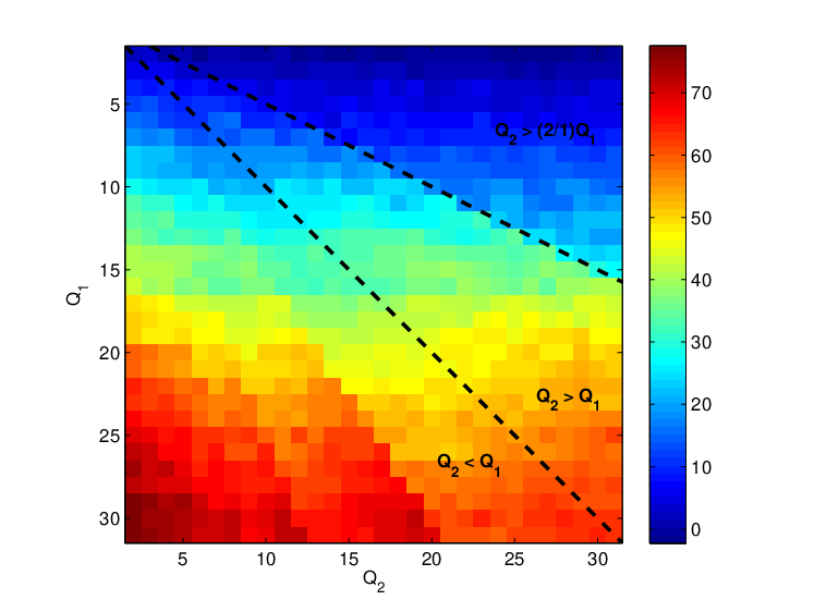
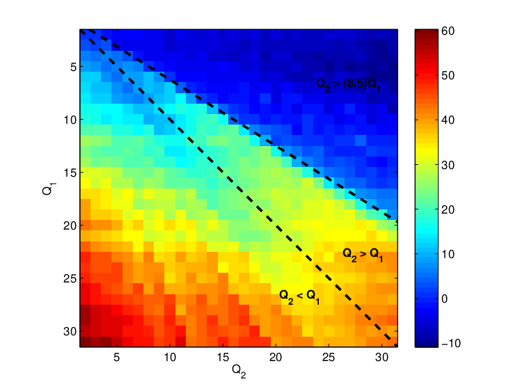
Once modeled and discussed all the terms in (12), we finally compare in Fig. 6 the resulting synthetic versions of the difference $\text{Var}\left(\mathbf{W}_{n}\right)|_{n\in\mathsf{I}_{1}}-\text{Var}\left(\mathbf{W}_{n}\right)|_{n\in\mathsf{P}_{1}}$ for the considered values of $\alpha_{\text{I}}$ (upper panels) with the ones empirically obtained after processing 14 videos from [8]⁴⁴ 4 In particular, we considered the following 14 CIF resolution videos: akiyo, bridge-close, bridge-far, container, foreman, hall, highway, mother-daughter, mobile, news, silent, paris, and waterfall. (lower panels). The synthetic models show a very high degree of similarity with respect to their empirical counterparts, except for the case $\alpha_{\text{I}}\!=\!2$, where the model possibly needs some adjustment. Still, this allows us to predict the strength of the VPF under each particular configuration of $\alpha_{\text{I}}$ and $\alpha_{\text{P}}$, and also to infer from which relation between $\text{Q}_{1}$ and $\text{Q}_{2}$ the VPF is more likely to show up or not. In this sense, the limits in the correlation maps previously discussed in the two above points, show the boundary beyond which the difference $\text{Var}\left(\mathbf{W}_{n}\right)|_{n\in\mathsf{I}_{1}}-\text{Var}\left(\mathbf{W}_{n}\right)|_{n\in\mathsf{P}_{1}}$ drops and, as a consequence, the VPF vanishes. In particular, we have seen that for $\alpha_{\text{I}}\in\{1,\frac{5}{4}\}$, this limit is achieved at $\text{Q}_{2}>(2/\alpha_{\text{I}})\text{Q}_{1}$ (see Figs. 6(a2)-(b2)), while it moves downward to $\text{Q}_{2}>(3/2)\text{Q}_{1}$ for $\alpha_{\text{I}}=\alpha_{\text{P}}$, as can be observed in Fig. 6(c2). Given that in all cases, the limit is above $\text{Q}_{2}>\text{Q}_{1}$, this explains why the VPF-based approaches are able to satisfactorily work in the challenging video forensic scenarios where the second compression applied is stronger than the first one. The reader is referred to [1] for checking how this theoretical analysis serves to predict the performance of the VPF-based methods.

References

- [1] D. Vázquez-Padín and F. Pérez-González, “Prediction residue analysis in MPEG-2 double compressed video sequences,” in Proceedings of the 27th European Signal Processing Conference (EUSIPCO), Sept 2019.
- [2] D. Vázquez-Padín, M. Fontani, T. Bianchi, P. Comesaña, A. Piva, and M. Barni, “Detection of video double encoding with GOP size estimation,” in Proc. of the 4th IEEE International Workshop on Information Forensics and Security (WIFS), December 2012, pp. 151–156.
- [3] D. Vázquez-Padín, M. Fontani, F. Pérez-González, D. Shullani, A. Piva, and M. Barni, “Video integrity verification and GOP size estimation via generalized variation of prediction footprint,” IEEE Transactions on Information Forensics and Security, 2019 (under review).
- [4] [Online]. Available: http://ffmpeg.org/
- [5] E. Y. Lam and J. W. Goodman, “A mathematical analysis of the DCT coefficient distributions for images,” IEEE Transactions on Image Processing, vol. 9, no. 10, pp. 1661–1666, Oct 2000.
- [6] G. Sullivan and T. Wiegand, “Rate-distortion optimization for video compression,” Signal Processing Magazine, IEEE, vol. 15, no. 6, pp. 74–90, 1998.
- [7] F. Bellifemine, A. Capellino, A. Chimienti, R. Picco, and R. Ponti, “Statistical analysis of the 2D-DCT coefficients of the differential signal for images,” Signal Processing: Image Communication, vol. 4, no. 6, pp. 477 – 488, 1992.
- [8] [Online]. Available: https://media.xiph.org/video/derf/