$SU(3)$ fermions in a three-band Graphene-like model

Geometric phases and related concepts have proved invaluable in understanding quantum mechanical phenomena which depend on the analytic structure of a parameterized Hilbert space, ranging from magneto-electric phenomena to topological insulators.Vanderbilt 2018; Xiao et al. 2010 Another striking domain is the quantum Hall effect that has been very instructive to modern condensed matter.Xiao et al. 2010 For weakly correlated electrons, they manifest in the Hilbert space of the Bloch wavefunctions of a band solid, where the parameter is the reciprocal crystal momentum. Berry phase is routinely used to such quantify geometric phases.Berry 1984 There are other quantifiers as well, e.g. the famous TKNN invariant is used in integer quantum Hall effect to quantify the geometric phase structure of filled gapped bands.Thouless et al. 1982

A very familiar example of a Berry phase effect in two dimensions (2$d$) is that of Graphene. Vafek and Vishwanath 2014 The Dirac cone spectra associated with mono-layer Graphene has a non-trivial geometric phase structure for each cone. Specifically, there is a Berry phase of $e^{i\pi}$ when one circuits around the cone. In presence of magnetic field and consequent Landau level formation, this structure can manifest sometimes as new Hall conductance plateaus. Zhang et al. 2006 Multi-layer Graphene Novoselov et al. 2006 is another example that hosts other multiples of $\pi$ Berry phases around its Dirac-like degeneracies.

For the above examples, there is an argument going back to Berry’s original article Berry 1984 that shows why we get multiples of $\pi$ (rather half-integral multiples of $2\pi$). When one considers the most general Hamiltonian that can characterize any two-fold degeneracy as happens in Dirac-like degeneracies, one obtains a $SU(2)$ matrix $H=\sum_{i\in\{1,2,3\}}\lambda_{i}\hat{\sigma_{i}}$. SU2 a The geometric phase in this case, is half the solid angle subtended by the circuit in the parameter space at the degeneracy point. Since in the preceding we have in general three parameters, for a non-fine-tuned degeneracy as a function of $2d$ crystal momentum in a $2d$ Bloch Hamiltonian, we need symmetries to reduce down to two parameters.gra Once so restricted to two parameters, we can only get multiples of $\pi$. This is the usual Dirac-like geometric phase structure in two dimensions.

The above argument motivates the starting point of this paper. Can there be two-dimensional non-interacting electronic band structures that host non-Dirac geometric phase structures? Since we have just argued that this possibility is absent for two-fold degeneracies, we have to look beyond them. The simplest generalization can then be a three-fold degeneracy. Thus we start by writing down a natural three-band generalization of the Dirac cone continuum Hamiltonian (Eq. 3). We find that this particular generalization indeed hosts a more intricate geometric phase structure than the two-fold Dirac cone wavefunctions. Even at the level of the spectrum, there are two-fold line-degeneracies that emanate from the three-fold degenerate point in the parameter space. Because of these line-degeneracies, and thereby a lack of adiabaticity in the usual sense Berry 1984, computing Berry phase around the three-fold degeneracy is formally problematic. lin

This leads us to describe this geometric phase structure using a triplet of indices which tracks how many times each member of the triplet (parameter, the Hamiltonian, the eigenfunctions) individually wind back to themselves as the system winds back to itself once, as we keep circuiting around the degeneracy point. Here, by the system, we mean the collection of the parameters, the Hamiltonian and all eigenfunctions. For our purpose, it proves useful to employ this method to classify the geometric phase structure near a multi-fold degenerate point in 2$d$ especially in the presence of line-degeneracies. This quantifier may be thought of as a conceptual generalization of the pseudospin winding number. Park and Marzari 2011

Analyzing this toy model further from the point of view of what space symmetries can guarantee this kind of a three-fold degeneracy, we find an interesting $SU(3)$ group structure near the three-fold degeneracy. It turns out that the above mentioned beyond-Dirac-like geometric phase structure obtains at fine-tuned points. Away from them, we get novel three-band Dirac-cone spectra that are a consequence of being “adiabatically” connected to this kind of three-fold degeneracy that we have found. We go on to write a tight-binding model which is hosted on a hexagonal lattice similar to Graphene but with three basis sites per unit cell. This still preserves the $SU(3)$ structure near three-fold degenerate points, now with an additional valley index arising similar to Graphene. Curiously the two-fold line degeneracies mentioned before connect the two valleys on a non-contractible loop in the Brillouin zone.

As a contrast to the toy model introduced above, we consider another simple three-band generalization of the Dirac cone as in Eq. 5 with a three-fold degeneracy. For this case, one again finds a Dirac-like geometric phase structure. This kind of three-fold degeneracy can be thought of as being in the spin-1 representation of $SU(2)$, which is again why we get Berry phase that are multiples of $\pi$. Thus, the $SU(3)$ structure of our toy model is intimately related to its non-Dirac-like geometric phase structure. Classifying non-trivial multi-fold degeneracies in electronic band structure as representations of certain groups (constrained by space symmetries) is a powerful point of view. Lin and Liu 2015; Bradlyn et al. 2016 In $2d$, there are several works which have considered three-fold degeneracies. Green et al Green et al. 2010 considered band structures resulting from putting microscopic fluxes in the hexagonal and Kagome lattices where they found a three-fold degeneracy. Here the fermions are in the spin-1 representation of the $SU(2)$ group, but their primary motivation was to find flat band structures. Subsequently, many other cases of spin-1 $SU(2)$ three-fold degeneracies have been reported. Dóra et al. 2011; Lan et al. 2011; Urban et al. 2011; Wang et al. 2013; Raoux et al. 2014; Giovannetti et al. 2015; Palumbo and Meichanetzidis 2015; Xu and Duan 2017; Wang and Yao 2018 Ref. Raoux et al. 2014’s $\alpha$-$\mathcal{T}_{3}$ model on the Dice lattice is noteworthy because it accommodates an interpolation between spin-$\frac{1}{2}$ and spin-1 Dirac fermions. We also note that in $3d$ which is not our focus, three-fold degeneracies have garnered tremendous interest recently, where they have been sometimes dubbed as triple point fermions. Lv et al. 2017; Winkler et al. 2016; Weng et al. 2016a; Zhu et al. 2016; Weng et al. 2016b; Chang et al. 2017a; Fulga and Stern 2017; Chang et al. 2017b; Zhong et al. 2017; Yu et al. 2017; Zhang et al. 2017; Yang et al. 2017 All these cases correspond to fermions being in the spin-1 representation of $SU(2)$ in the majority (however, see Ref. Chang et al. 2017a for an example where the geometric phase structure goes beyond Weyl/Dirac in 3$d$).

In our $2d$ toy model, unlike the above, the fermions are in the fundamental representation of the $SU(3)$ group. Going away from this fine-tuned model, we get multiple two-fold Dirac cones for generic directions and a three-fold point-degeneracy for some fine-tuned directions. But the $SU(3)$ nature of the toy model manifests itself in the way the various two-fold and three-fold degeneracies are organized to accommodate the $SU(3)$ geometric phase structure. Thus, the presence of the fine-tuned $SU(3)$ point controls the various Dirac cone structures obtained in its vicinity.

The outline of the paper is as follows: In Sec. II, we write down a three-band generalization of the Dirac cone Hamiltonian, and discuss its beyond-Dirac geometric phase structure. In Sec. III, we study the construction of such generalizations using symmetries. This gives a family of three-band Hamiltonians where the fermions transform in the fundamental representation of $SU(3)$. In Sec. III.1, we categorize the band structures for various cases of this family of Hamiltonians. In Sec. IV, we give a lattice model realization of the above Hamiltonians, and a brief numerical study of the effect of uniform magnetic field on this non-interacting system. We conclude with a summary and outlook in Sec. V.

To set the stage, we recall that the low-energy physics of Graphene is obtained from a two-band lattice hopping model Wallace 1947; Vafek and Vishwanath 2014 which gives two distinct Dirac cones or valleys in the Brillouin zone of the underlying triangular Bravais lattice. Our convention is to choose the location of valleys as $\mathbf{K}=\left(\frac{4\pi}{3},0\right)$ and $\mathbf{K}^{\prime}=\left(-\frac{4\pi}{3},0\right)$ (unit length is set by separation between two neighboring unit cells, and $\mathbf{K}$, $\mathbf{K}^{\prime}$ are related by a reflection across the $y$-axis). Near one of these valleys in energy units of $\hbar v_{F}=1$, one can write down the familiar continuum Hamiltonian

where $\mathbf{p}$ is the expansion variable near $\mathbf{K}$ with the full crystal momentum being $\mathbf{K}+\mathbf{p}$. Its eigensystem is

where $p=\sqrt{p^{2}_{x}+p^{2}_{y}}$, and $\theta_{\mathbf{p}}=\arctan\left(\frac{p_{y}}{p_{x}}\right)$. This gives the familiar Berry phase of $e^{i\pi}$ as the parameter $\mathbf{p}$ (and thereby the angular variable $\theta_{\mathbf{p}}$) winds around once about the two-fold degenerate point. We note here that during this winding, the full system – comprising the parameter $\mathbf{p}$, the Hamiltonian $H^{\text{Dirac}}_{K}(\mathbf{p})$, and all eigenvectors $\{v_{i}(\mathbf{p})\}$ – winds around once as well.

Now, we come to our primary object of interest in this paper. Consider the following three-band generalization of the continuum Dirac Hamiltonian $H^{\text{Dirac}}_{K}(\mathbf{p})$ recalled above,

where the subscript $K$ refers again to a valley index anticipating the lattice model realization of the above in Sec. IV. The eigensystem of $H^{3A}_{K}(\mathbf{p})$ is

where $\omega=e^{i\frac{2\pi}{3}}$, $\omega^{2}=e^{-i\frac{2\pi}{3}}$ are the complex cube roots of unity.

The dispersion near the three-fold degeneracy is shown in Fig.1 and Fig. 2 (for fixed $p=1$). It is linear in $p$ similar to a Dirac cone, however, now there are a pair of two-fold line degeneracies that emanate from the three-fold degeneracy outwards in the opposite directions along the $p_{x}$-axis. This already gives us a sense of the non-Dirac geometric phase structure of $H_{K}^{3A}$.

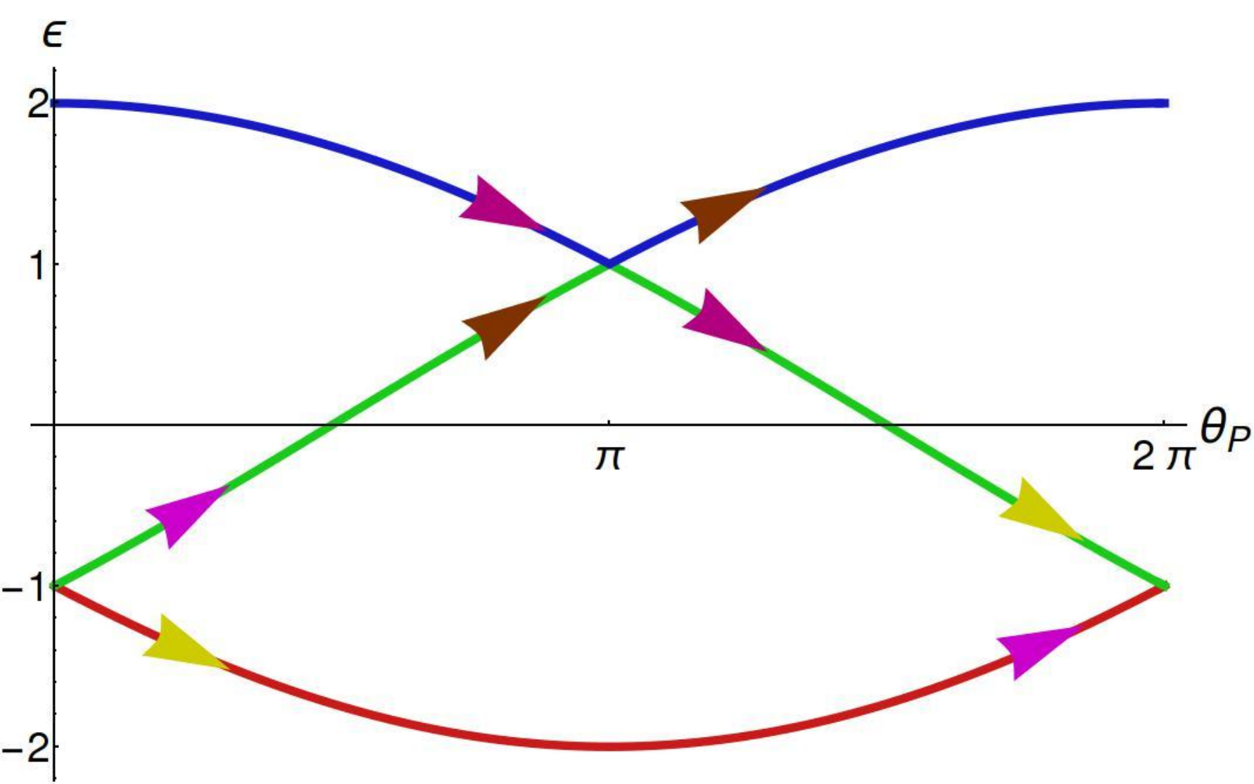
The source of the non-Dirac geometric phase structure actually lies in the $e^{i\theta_{\mathbf{p}}/3}$ and $e^{i2\theta_{\mathbf{p}}/3}$ terms in $H^{3A}_{K}$’s eigensystem Eq. 4. The analytic structure of these terms is qualitatively different than $e^{i\theta_{\mathbf{p}}}$ that appears in the eigensystem of $H^{\text{Dirac}}_{K}$. $z=re^{i\theta}$ is an analytic function everywhere on the complex plane, whereas $z^{1/3}=r^{1/3}e^{i\theta/3}$ has branch-cuts in the complex plane, and needs three Riemann surfaces to embed the function in an analytic way. The two-fold line degeneracies in Fig. 1 are representing these branch-cuts in the following way: we can rewrite the eigenvalues as $\bigg\{\epsilon_{1}^{3A}(\mathbf{p})=2p\>\text{Re}\left[\omega^{2}\sqrt[3]{e^{i\theta_{\mathbf{p}}}}\right],\epsilon_{2}^{3A}(\mathbf{p})=2p\>\text{Re}\left[\sqrt[3]{e^{i\theta_{\mathbf{p}}}}\right],$ $\epsilon_{3}^{3A}(\mathbf{p})=2p\>\text{Re}\left[\omega\sqrt[3]{e^{i\theta_{\mathbf{p}}}}\right]\bigg\}$ which are essentially the Riemann surfaces of the complex cube root. We also show this in a different way in Fig. 2 through pairs of colored arrows which indicate the rule to move among the bands across the line degeneracies in order to move in an analytically smooth way.

To quantify the geometric phase structure of $H_{K}^{3A}$, we can not use Berry phase straightforwardly due to the line degeneracies which present obstructions while doing a circuit in the parameter space around the three-fold degeneracy. However, from the above discussion, we see that to move in an analytically smooth way, we have moved across bands as shown in Fig. 2 as we make circuits around the three-fold degeneracy. This figure also shows that to analytically return back to the starting point in energy (modulo $p$) at a non-degenerate point, we have to circuit three times around the degeneracy. During these three circuits, one may easily check that the Hamiltonian (Eq. 3) returns back to itself thrice as well, while the wavefunctions return back to themselves only twice via Eq. 4.

This motivates the following triplet of indices to characterize the geometric phase structure around any two-dimensional multi-fold degeneracy. We track how many times the parameter ($\theta_{\mathbf{p}}$), the given Hamiltonian, and all eigenfunctions $v^{i}(\theta_{\mathbf{p}})$ return to themselves, as we perform a single circuit around the degeneracy for the full system comprising the parameter, the Hamiltonian, and all eigenvectors. This triplet of indices tracking the individual windings is a quantifier of the geometric phase structure near the degeneracy. This is summarized in Table 1 for several different two-fold and three-fold degenerate systems. We see from this table how our three-band model has a non-trivially different geometric phase structure than the other cases which are all Dirac-like. Thus our model is an example of a beyond-Dirac geometric phase structure in two dimensions. It can also be checked that $\left(\begin{matrix}0&p_{x}-ip_{y}&p_{x}-ip_{y}\\ p_{x}+ip_{y}&0&p_{x}-ip_{y}\\ p_{x}+ip_{y}&p_{x}+ip_{y}&0\end{matrix}\right)$ has the same kind of beyond-Dirac geometric phase structure as $H_{K}^{3A}$.

Our three-band continuum Hamiltonian can be contrasted with a Dirac-like three-band case with a three-fold degeneracy of the following form

Its eigensystem is

As is evident from the eigensystem above, this case has no branch cut structure and no line degeneracies. It can, in fact, be shown that the geometric phase structure, in this case, is still Dirac-like similar to $H_{K}^{\text{Dirac}}$ but in a three-fold situation. SU2 b We also note how it contrasts with beyond-Dirac-like $H_{K}^{3A}$ in Table 1. In all of the above, we have fixed our gauge by choosing the last entry of the wavefunctions’ column vectors to be purely real. The classification in Table 1 is independent of this gauge choice, since wavefunctions differing by pure phases are physically equivalent and have the same windings around degeneracies.

In this section, we expose the underlying $SU(3)$ group structure in Eq. 3 as remarked in Sec. I. To set the stage, we remind ourselves that for monolayer Graphene with two-fold degeneracies, a continuum Hamiltonian can be written using the Pauli matrices ($SU(2)$ generators in fundamental representation) near the degeneracy points in the Brillouin zone. It is obtained by expanding around the $\mathbf{K}$ and $\mathbf{K^{\prime}}$ points in the Brillouin zone of Graphene and looks like

where $\hat{c}^{\dagger}_{\mu\alpha},\hat{c}_{\mu\alpha}$ are the fermion creation and annihilation operators for the so-called valley index $\mu\in{\mathbf{K},\mathbf{K^{\prime}}}$ and sublattice index $\alpha\in{a,b}$, and

and $\tau^{i}$ are $SU(2)$ Pauli matrices indexing the two valleys, $\sigma^{i}$ are $SU(2)$ Pauli matrices indexing the two sub-lattices of the Graphene lattice, $\mathbf{p}$ is the expansion variable (i.e. the full crystal momentum is $\mathbf{k}=\mathbf{K}+\mathbf{p}$, etc.), and all the indices have been shown explicitly. We can rewrite Eq. 8 concisely by dropping the explicit indices as $H^{\text{Dirac}}=p_{x}\left(\tau^{3}\otimes\sigma^{1}\right)+p_{y}\left(\tau^{0}\otimes\sigma^{2}\right)$. In this way of saying, our three-band continuum Hamiltonian written down in the previous section in Eq. 3 actually requires all the off-diagonal generators of the $SU(3)$ group, i.e.

where we use the Gell-Mann matrices as the $SU(3)$ generators. Halzen and Martin 1984 On the other hand, spin-1 generators of the $SU(2)$ group – which are a subset of the $SU(3)$ group generators – suffice for the Hamiltonian in Eq. 5 ,

This leads us to ask the following question: Along with time-reversal symmetry, what are the spatial point group symmetries that we want to preserve while constructing a general continuum Hamiltonian in two dimensions which has the above $SU(3)$ group structure? In the case of Graphene, the spatial point group symmetries of $\mathcal{C}_{3}$ ($2\pi/3$ rotation about the center of a hexagonal plaquette), $\mathcal{C}_{2}$ (inversion, or equivalently a $\pi$ rotation about the center of a hexagonal plaquette) and $\mathcal{P}_{x}$/$\mathcal{P}_{y}$ (reflections about axes passing through the center of a hexagonal plaquette) are sufficient to constrain us in writing down Eq. 8 as the general continuum Hamiltonian that preserves these symmetries.

For our model, we will start by considering a $\mathcal{C}_{2}$ symmetry. The generic operation of the $\mathcal{C}_{2}$ can be taken to be as follows: one sublattice remain unchanged, while the other two sublattices get interchanged (e.g. $a\rightarrow b$, $b\rightarrow a$, $c\rightarrow c$). This operation thus looks like

where

and we stick with $a\rightarrow b$, $b\rightarrow a$, $c\rightarrow c$ convention as in example above. However this choice is not special, and all other conventions – that interchange two sublattices and keep one sublattice unchanged – will give us the same spectrum. $\mathbf{p}\rightarrow-\mathbf{p}$ in the above because the full crystal momentum changes sign, i.e. $\mathbf{k}=\mathbf{K}+\mathbf{p}\rightarrow-\mathbf{k}=-\mathbf{K}-\mathbf{p}=\mathbf{K}^{\prime}-\mathbf{p}$, which is essentially the $\tau^{1}$ operation in the valley index, and $\mathbf{p}\rightarrow-\mathbf{p}$ for the fermion operators.

We can easily check the following identities for the $C_{2}$ matrix ($=C^{-1}_{2}$) that implements $\mathcal{C}_{2}$,

At the outset, the list of possible terms are of the form $f_{ij}(\mathbf{p})\>\tau^{i}\otimes\Lambda^{j}$ where $f_{ij}(\mathbf{p})$ is some real function of $\mathbf{p}$. For local Hamiltonians, we can remove terms in this list which contain $\tau^{1}$ or $\tau^{2}$. So the generic local Hamiltonian that is invariant under $\mathcal{C}_{2}$ must be a combination from a reduced list of terms, e.g. terms that contain $\Lambda^{1}$ will be of the form

where the superscripts are used designate whether the function is even or odd, i.e. $f^{\pm}_{ij}(-\mathbf{p})=\pm f^{\pm}_{ij}(\mathbf{p})$. We quickly discuss the reason that governs the even/odd property of the above functional coefficients $f^{-}(\mathbf{p})$ and $f^{+}(\mathbf{p})$. This is a standard argument that is used for Graphene as well. We will do it for the case of $\tau^{0}\otimes\Lambda^{1}$ as an example.

Under $\mathcal{C}_{2}$ we have $\tau^{0}\rightarrow\tau^{0}$. Thus using Eq.13a, $\tau^{0}\otimes\Lambda^{1}\rightarrow\tau^{0}\otimes\Lambda^{1}$. Then (from here on, we suppress indices unless needed)

Thus $\mathcal{H}^{3A}$ remains invariant if $f^{+}(-\mathbf{p})=f^{+}(\mathbf{p})$. All the other possible terms can be analyzed in a similar way. The full list of terms that are finally allowed by $\mathcal{C}_{2}$ following the above considerations are

All odd functions in $\mathbf{p}$ at leading order will be linear in $p_{x},p_{y}$, and all even functions in $\mathbf{p}$ at leading order will be constants. We are mainly interested in these leading order behaviors. We will comment on higher order terms when needed.

Next, we consider time reversal symmetry $\mathcal{T}$. Time reversal operation looks like

(and $\mathcal{T}\>i\>\mathcal{T}^{-1}=-i$). The list of terms allowed by time reversal symmetry (following the same steps as $\mathcal{C}_{2}$) are

Finally, we consider reflection symmetries, $\mathcal{P}_{x}$ about $y$-axis and $\mathcal{P}_{y}$ about $x$-axis. Their combined operations implements $\mathcal{C}_{2}$ in two dimensions, i.e. $\mathcal{P}_{x}\mathcal{P}_{y}=\mathcal{C}_{2}$. Now we know from Eq. 11 that $\mathcal{C}_{2}$ implements both $\tau^{1}$ (valley exchange) and $C_{2}$ ($a\leftrightarrow b$, $c\leftrightarrow c$). So the non-trivially different symmetry operations that $\mathcal{P}_{x}$/$\mathcal{P}_{y}$ can do are that one of them implements valley exchange, and the other implements $C_{2}$. Also, we note that under $\mathcal{P}_{x}$, $\mathbf{K}\leftrightarrow\mathbf{K}^{\prime}$ and under $\mathcal{P}_{y}$, $\mathbf{K}$/$\mathbf{K}^{\prime}$ remain unchanged for our choice of the valley locations in the Brillouin zone. Therefore, $\mathcal{P}_{x}$ implements valley exchange with the sublattices unchanged, and $\mathcal{P}_{y}$ implements $C_{2}$ with the valleys unchanged. Thus, $\mathcal{P}_{x}$/$\mathcal{P}_{y}$ operations look like

Also, because $\mathcal{P}_{x}(\mathbf{k})=(-k_{x},k_{y})$ and $\mathbf{K}\leftrightarrow\mathbf{K}^{\prime}$ under $\mathcal{P}_{x}$, therefore $\mathcal{P}_{x}(\mathbf{p})=(-p_{x},p_{y})$ as well. Similarly, $\mathcal{P}_{y}(\mathbf{p})=(p_{x},-p_{y})$.

Now we explicitly redo the similar analysis as for $\mathcal{C}_{2}$ for one term $g^{+}(\mathbf{p})\tau^{3}\otimes\Lambda^{2}$ as an example.

Thus at the leading order $g^{+}(\mathbf{p})$ will be zero, but higher order terms such $p_{x}p_{y}$ will satisfy the relation $g^{+}(\mathcal{P}_{x}(\mathbf{p}))=-g^{+}(\mathbf{p})$ and are thus allowed. Similarly $m^{+}_{2}(\mathbf{p})$ is zero at leading order. Therefore, all the terms in Eq. 18 in principle are allowed by reflections, but restricting up to leading order, the Hamiltonian looks like

In the above, all the function symbols are now replaced by constants. This Hamiltonian for $n^{-}=n^{+}=f^{+}=l_{1}^{+}=0$ and $f^{-}=l^{-}_{1}=g^{-}=m_{2}^{-}\neq 0$ is Eq. 3. As discussed in Sec. II, Eq. 3 has a three-fold degeneracy and two two-fold line degeneracies emanating from it (See Fig.1).

In this section, we write down a Graphene-like lattice fermion model motivated by the plausibility of realizing the continuum Hamiltonians described in previous sections, Eq. 3 and 21, in some real-world material. The lattice that we consider is shown in Fig. 9. It is chosen to be very similar to the Graphene lattice with an extra lattice site in the middle of vertical bonds. On this lattice, apart from the conventional hopping matrix elements as in Graphene between $a$ to $b$ sublattices, we also include hopping matrix elements between $a$ and $c$ sublattices as well as $b$ and $c$ sublattices. We note that the geometric distance between $a$-$c$ and between $b$-$c$ inside the same unit cell is smaller than between $a$-$b$. For inter-unit cell hoppings, the situation is the opposite. So generically these hopping strengths are not equal. This lattice model can either be thought of as a planar model, or a two-layer model where one of the layers is hexagonal and the other layer is triangular. Thus, the $c$ sublattice sites are not symmetry related to the $a,b$ sublattice sites. The $a,b$ sublattice sites may be related by either a $\mathcal{C}_{2}$ rotation symmetry with any $c$ site as the rotation center, or by a reflection around an axis form by joining a horizontal row of $c$ sites.

The hopping Hamiltonian that we consider on this graphene-like lattice going by the above symmetry considerations is given by Eq. 23, where $n_{1},n_{2}$ are unit-cell indices using the primitive lattice vectors of the underlying triangular lattice. Here, we are not considering staggered potentials, whose effect is discussed in section III.1 (in particular case 5: $n^{+}\tau^{0}\otimes\Lambda^{8}$; a term like $\tau^{0}\otimes\Lambda^{3}$ is ruled out by $\mathcal{C}_{2}$).

This lattice Hamiltonian clearly reproduces the continuum $H_{\mu}^{\text{3A}}$ band structure near the valleys $\vec{K},\vec{K}^{\prime}$ when the “deformations” $\delta t_{0}$ and $\delta t_{1}$ are zero as may be seen by expanding to leading order near these points in the zone. Essentially they are three copies of Graphene hoppings with the same strength. The dispersion over the full Brillouin zone for this choice of parameters is shown in the left panel of FIG.10. The two-fold line degeneracies that connect the two valleys $\vec{K},\vec{K}^{\prime}$ form a non-contractible loop in the Brillouin zone. This is shown in the right panel of FIG.10.

For generic deformations, $\delta t_{0}\neq 0$, $\delta t_{1}\neq 0$, the two-fold line degeneracies go away. Then, the continuum Hamiltonians near the two valleys look like

This deformed Hamiltonian is in the form found in Sec. III, Eq. 21 consistent with all our symmetry considerations. We reiterate that for our lattice hopping model, we have $n^{+}=n^{-}=f^{+}=0$ in the notation of Sec. III. The reasons are as follows: a) $n^{+}$ and $n^{-}$ are zero because there are no staggered chemical potentials and no inter-cell same sublattice hoppings. b) $f^{+}=0$ because we are measuring deformations in hopping with respect to $ab$ hoppings within the unit cell. Secondly, $l^{+}_{1}\neq 0$ is the way we chose to organize the deformations due to $\delta t_{0}$, $\delta t_{1}$ as shown in Eq. 24 and 25. Therefore, the rest of the Hamiltonian is the undeformed case, which makes $f^{-}=g^{-}$ and $m_{2}^{-}=l_{1}^{-}$. In fact, $f^{-}=g^{-}$ is precisely what happens in Graphene.

The band structure for this generic case ($\delta t_{0}\neq\delta t_{1}\neq 0$) near the valleys is shown in Fig. 11. We find that the bottom two bands touch linearly as in a Dirac cone, while the middle and the top band involve two Dirac cones. The dispersion along the line connecting the two Dirac cones is rather flat. This is basically the lattice realization of case 3 in Sec. III where the line connecting the two Dirac cones is completely flat. The lack of complete flatness for the lattice case is due to subleading terms.

For the middle and bottom band, there can in fact be another Dirac cone apart from the one mentioned above, which can annihilate with a similar counterpart from the other valley as we tune $\delta t_{1}$ for a given $\delta t_{0}$ as shown in Fig. 12. This happens when $\delta t_{1}$ and $\delta t_{0}$ are of the same sign. When their signs are opposite, they are always annihilated as shown in Fig. 13. In our Graphene-like lattice, we expect the opposite sign case to be the physical case if we assume that hopping strength decreases with distance.

We also mention a fine-tuned case of deformation when $\delta t_{0}=\delta t_{1}\neq 0$. The corresponding band structure near the valleys is included in case 2 in Sec. III where we again have a three-fold degeneracy without two-fold line degeneracies. A final comment on breaking the $\mathcal{C}_{2}$ symmetry and thereby opening gaps near the Dirac cones: this makes the gapped bands topologically trivial bands with zero Chern number just like Graphene.