NIHAO XXII: Introducing black hole formation, accretion and feedback into the NIHAO simulation suite2019NIHAO XXII: Introducing black hole formation, accretion and feedback into the NIHAO simulation suite–1
Abstract
We introduce algorithms for black hole physics, i.e., black hole formation, accretion and feedback, into the NIHAO (Numerical Investigation of a Hundred Astrophysical Objects) project of galaxy simulations. This enables us to study high mass, elliptical galaxies, where feedback from the central black hole is generally thought to have a significant effect on their evolution. We furthermore extend the NIHAO suite by 45 simulations that encompass halo masses from to , and resimulate five galaxies from the original NIHAO sample with black hole physics, which have halo masses from to . Now NIHAO contains 144 different galaxies and thus has the largest sample of zoom-in simulations of galaxies, spanning halo masses from to . In this paper we focus on testing the algorithms and calibrating their free parameters against the stellar mass versus halo mass relation and the black hole mass versus stellar mass relation. We also investigate the scatter of these relations, which we find is a decreasing function with time and thus in agreement with observations. For our fiducial choice of parameters we successfully quench star formation in objects above a halo mass of , thus transforming them into red and dead galaxies.
Keywords:
methods: numerical – galaxies: active – galaxies: evolution – galaxies: formation – galaxies: nuclei – quasars: general.1 Introduction
It is now well established that black holes exist in the centres of almost all galaxies (Kormendy & Richstone 1995; Magorrian et al. 1998, e.g.,), and that they are connected to their hosts. The general idea outlined by Di Matteo et al. 2005 is that feedback provided by the central black hole heats the galaxy’s gas and subsequently quenches star formation and further black hole accretion, transforming it into a ‘red and dead’ elliptical galaxy. In this framework this co-evolution leads the galaxy, i.e. its velocity dispersion (Ferrarese & Merritt 2000; Gebhardt et al. 2000, e.g.,) or its bulge mass (Kormendy & Richstone 1995; Häring & Rix 2004, e.g.,), being related to the black hole mass. However, some works (Jahnke & Macciò 2011, e.g.,) argue that correlations between the galaxy and its central black hole do not imply a physical connection of these two.
Numerical simulations have been proven very successful in investigating the formation and evolution of galaxies, leading to a number of projects that have been developed over the last years. E.g., Illustris (Vogelsberger et al. 2014), IllustrisTNG (Pillepich et al. 2018), Magneticum Pathfinder (Dolag et al. 2016), MassiveBlack-II (Khandai et al. 2015) and EAGLE (Schaye et al. 2015) are hydrodynamic simulations of cosmological volumes, and FIRE (Hopkins et al. 2014) and Auriga (Grand et al. 2016) consist of zoom-in simulations of individual galaxies.
The NIHAO project (Wang et al. 2015) is a suite of hydrodynamical cosmological zoom-in simulations of galaxies and is unique in combining (i) a high resolution of particles per halo, (ii) a large range of halo masses from dwarf to Milky Way masses ( to ), and (iii) a large sample size of 100 galaxies. NIHAO successfully reproduces the stellar mass versus halo mass relation, one of the most fundamental constraints in galaxy formation and evolution, from redshift up to redshift , and also matches the star formation rate versus stellar mass relation. However, up to this date the NIHAO suite did not include high mass, elliptical galaxies, because the stellar feedback implemented into NIHAO is insufficient to regulate star formation in elliptical galaxies (Dutton et al. 2015). It is now generally accepted (Croton et al. 2006) that black hole feedback is needed at higher masses to reproduce the sharp decline in the stellar mass function and to create red and dead galaxies.
The aim of this paper is to introduce algorithms for black hole formation, accretion and feedback into the NIHAO project, and to extend the NIHAO suite to include high mass, elliptical galaxies. We focus on the testing of the algorithms and the calibration of the free parameters on the observed stellar mass versus halo mass and black hole mass versus stellar mass relations, and also investigate how the scatter of these relations evolve with time and compare with observations. In section 2 we review the properties of the NIHAO project. We introduce the algorithms used for black hole formation, accretion and feedback in section 3 and the initial conditions in section 4. In section 5 we present our results and in section 6 we study the effect of the algorithms’ free parameters on the simulations. In section 7 we summarize our findings.
2 The NIHAO project
NIHAO uses an updated version (Keller et al. 2014) of the TreeSPH code Gasoline2 (Wadsley et al. 2004; Wadsley et al. 2017). The simulations use a flat LCDM cosmology with parameters from the Planck Collaboration et al. 2014.
The backbone of the NIHAO project consists of cosmological dark-matter-only simulations with box sizes of 60 and 20 Mpc/h from Dutton & Macciò 2014, and a new box of 15 Mpc/h with particles. These are evolved until , then haloes from these boxes are selected and resimulated individually with a higher resolution and with gas particles.
All galaxies have the same relative resolution across the whole mass range, i.e. dark matter particles inside the virial radius at . The particle masses and force softening lengths are chosen to resolve the mass profile at 1 per cent of the virial radius. The initial ratio of dark and gas particle mass equals the cosmological mass ratio of dark matter and baryons of . The softening length of gas and star particles is times smaller than the dark matter particle softening length. The free parameters of the stellar and supernova feedback model have been chosen to match the - relation for one Milky Way-like galaxy at .
Cooling is provided via hydrogen, helium, and various metal-lines in a uniform ultraviolet ionizing background (Shen et al. 2010), this includes photoionization, UV background heating (Haardt & Madau 2012), and Compton cooling.
Stars are formed from gas particles that pass a density and temperature threshold (, ) with a rate of , where is the gas particle’s dynamical time, its density, its mass and the star formation efficiency.
Supernova feedback is modeled with the blastwave formalism of Stinson et al. 2006. Stars of mass eject metals and energy to surrounding gas particles 4 Myr after their formation. For these gas particles cooling is delayed for . Before they produce a supernova massive stars provide ‘early stellar feedback’ (Stinson et al. 2013), i.e. 13 per cent of the total stellar flux of is injected into the surrounding gas as thermal energy. No cooling delay is applied in this case. We refer to Wang et al. 2015 for more details of the NIHAO project.
NIHAO has been very successful in reproducing galaxy properties for halo masses of , e.g., the stellar mass versus halo mass relation (Wang et al. 2015), the galaxy velocity function (Macciò et al. 2016), the Tully-Fisher relation (Dutton et al. 2017) and the rotation curves of dwarf galaxies (Santos-Santos et al. 2018).
3 Computational methods for black hole physics
Black holes are modeled as sink particles (Bate et al. 1995) that only interact with their environment via gravitational forces and that can accrete matter from neighboring gas particles. For black hole accretion and feedback we choose the models introduced by Springel et al. 2005, because these are the most widely used and thus tested, and are known to be able to yield the correct relation between black hole mass and the stellar component (Di Matteo et al. 2005).
3.1 Black hole formation
We follow a common approach for modeling black hole formation: when a central halo11 1 We do not seed subhaloes. exceeds a threshold mass we convert the gas particle (or a part thereof) with the lowest gravitational potential into a black hole with seed mass .22 2 E.g., Sijacki et al. 2007 use and M☉, Di Matteo et al. 2008 and Schaye et al. 2015 use and M☉, Schaye et al. 2010 use and and Sijacki et al. 2015 use and . Haloes and their masses are found with the AMIGA Halo Finder (Gill et al. 2004; Knollmann & Knebe 2009, AHF,), see section 4 for more details. We follow Sijacki et al. 2007 and use the values M☉ and . An alternative model for black hole formation is used in the Romulus simulations (Tremmel et al. 2017), where black hole formation occurs when the gas meets specific thresholds for metallicity, density and temperature.
3.2 Black hole relocation
In galaxy-scale simulations two effects can lead the position of the black hole not to coincide with the halo centre: (i) The small ratio of black hole mass and gas/star/dark particle mass leads to stochastic motions of the black hole particle caused by the momentum of the accreted gas and gravitational interactions with nearby particles. (ii) In the case of two haloes merging dynamical friction would lead the black hole to sink to the centre of the newly forming halo. However, in galaxy-scale simulations dynamical friction is generally underestimated on small scales due to insufficient resolution.
To compensate for these effects a number of models have been developed in the last years: Debuhr et al. 2011; Debuhr et al. 2012 and Anglés-Alcázar et al. 2017 assign the black hole a ‘dynamical mass’ or ‘tracer mass’, which is several orders of magnitude larger than the actual black hole mass, to prevent the black hole from moving too far away from the halo centre. Johansson et al. 2009 relocate the black hole to the gas particle within the SPH smoothing length of the BH that has the lowest gravitational potential. Booth & Schaye 2009 also relocate the black hole to the neighboring gas particle with the lowest gravitational potential, but only if the relative velocity of black hole and gravitationally most bound gas particle is smaller than 25 per cent of the local speed of sound and if the black hole mass is smaller than ten times the initial gas particle mass. The IllustrisTNG simulations (Sijacki et al. 2015) force the black hole particle to be located at the potential minimum of its host halo. The EAGLE simulations (Schaye et al. 2015) force black holes with a mass smaller than 100 times the gas particle mass to migrate towards the minimum of the gravitational potential of its host halo. The Magneticum Pathfinder simulations (Hirschmann et al. 2014) and the the Romulus simulations (Tremmel et al. 2017; Tremmel et al. 2015) include a subgrid model to account for the dynamical friction force that is acting on the black hole.
However, relocating the black hole to the potential minimum of its host halo can lead it to move very large distances (the sum of the haloes virial radii, i.e., several ) in the case of two haloes merging. Furthermore, if these two haloes, whose black holes have just merged, disconnect again, the halo that just lost its black hole would get re-seeded. To avoid these problems every major time step33 3 The simulation time of 13.8 Gyr is divided into 1024 major time steps of 13.4 Myr. we set the position and velocity of the black hole to the values of the dark matter particle within ten softening lengths that has the lowest gravitational potential. Using the star particle with the lowest gravitational potential might be problematic at high redshifts, when only few or no star particles are present. Placing the black hole at the gas particle with the lowest gravitational potential would artificially increase its kernel weight, thus its density and thus the black hole accretion rate. Furthermore, using a gas particle that has recently received feedback and is thus outflowing could lead to inappropriate black hole velocities and/or large jumps in the black hole position. (See Wurster & Thacker 2013, for a discussion of a similar problem.).
3.3 Black hole merging
Two black holes are merging when their distance is smaller than the sum of their softening lengths. The resulting black hole inherits the position, velocity and acceleration of its predecessors’ barycentre, its mass is the sum of its predecessors’ masses, and its accretion rate is calculated in the next timestep.
3.4 Black hole accretion
We calculate the accretion rate of the black hole with the commonly used44 4 E.g., in Di Matteo et al. 2005, Springel et al. 2005, Colberg & Di Matteo 2008, Di Matteo et al. 2008, Booth & Schaye 2009, Croft et al. 2009, Johansson et al. 2009, Choi et al. 2012. Bondi-Hoyle-Lyttleton parametrization (Hoyle & Lyttleton 1939; Bondi & Hoyle 1944; Bondi 1952)
| (1) |
where is the black hole mass and , and are the density, sound speed and velocity of the gas that surrounds the black hole. The parameter was first introduced by Springel et al. 2005 to account for the limited resolution of these simulations, and is usually set to (Booth & Schaye 2009, see, e.g., table 2 in). However, our resolution is higher than in earlier works that use the Bondi-Hoyle-Lyttleton parametrization, therefore we use an accretion parameter of and justify this choice with a parameter study in section 6.
The black hole accretion rate is limited by the Eddington rate (Eddington 1921)
| (2) |
with the Salpeter time-scale (Salpeter 1964) and the radiative efficiency (Shakura & Sunyaev 1973). The black hole accretion rate then is
| (3) |
At each time step the black hole accretes the mass from the gas particle(s) that is (are) most gravitationally bound to the black hole. The momentum of the accreted mass is added to the black hole’s momentum. The black hole can accrete fractions of a gas particle, which might lead to gas particles with a very small mass. If a gas particle’s mass falls below 20 per cent of its initial mass it is deleted and its mass and momentum are distributed among the surrounding gas particles weighted with the SPH kernel.
To avoid too large accelerations and thus too small time steps of particles close to the black hole, as well as two body relaxation, we increase the black hole softening length as it grows. As the softening length of collisionless particles in our simulations is proportional to the square root of their mass, we multiply the black hole softening length with when it increases by in mass.
Increasing the softening length of the black hole does not significantly affect its surroundings, as its gravitational force is usually much smaller than the gravitational force of the stars surrounding the centre. E.g., for the galaxy g7.92e12 that we use for our parameter study in section 6, the mass of the stars within of the black hole is at least 25 times larger than the mass of the black hole for all times.
We do not limit how far particles can be away in order to be accreted. However, usually in each timestep not more than one particle is accreted, and this one is the most bound one, and thus usually the closest to the black hole.
Alternative methods to model gas accretion onto black holes have been developed: Booth & Schaye 2009; Booth & Schaye 2010 assume that the accretion parameter is not constant, but a function of the gas density, whereas in the EAGLE simulations (Schaye et al. 2015) and Rosas-Guevara et al. 2015 is the ratio of Bondi time-scale and viscous time-scale. Tremmel et al. 2017 modify the Bondi-Hoyle-Lyttleton parametrization to take the angular momentum of the gas into account. Debuhr et al. 2011; Debuhr et al. 2012 calculate the black hole accretion rate based on the viscous evolution of an accretion disc that surrounds the black hole. Hopkins & Quataert 2011 and the FIRE simulations (Anglés-Alcázar et al. 2017) calculate the black hole accretion rate based on angular momentum and gravitational torques around the black hole.
3.5 Black hole feedback
Black hole accretion results in a luminosity of
| (4) |
with speed of light , and we assume that a fraction55 5 Common values for the feedback efficiency are (Di Matteo et al. 2005; Springel et al. 2005; Sijacki et al. 2007; Di Matteo et al. 2008; Johansson et al. 2009), (Booth & Schaye 2009; Booth & Schaye 2010; Schaye et al. 2015) and (Tremmel et al. 2017). of this luminosity is available as thermal energy for the gas that surrounds the black hole. Thus the gas receives an energy per time of
| (5) |
that is distributed kernel weighted among the 50 nearest gas particles. To avoid too large sound speeds and thus too small time steps we limit the specific energy of a single gas particle to .
There are a few alternative models for black hole feedback. Sijacki et al. 2007 use an additional feedback mode operating at low black hole accretion rates that is modeled by injecting ‘bubbles’ into the host galaxy. Debuhr et al. 2011; Debuhr et al. 2012 and Choi et al. 2012 use ‘kinetic feedback’ that feeds momentum and mass to the gas surrounding the black hole.
4 Initial conditions, galaxy properties and parameters
Our galaxies and their properties are listed in Table 1 at the end of this paper. We take five galaxies from the original NIHAO suite that have a dark matter particle mass of , a gas particle mass of , a dark matter softening length of and a gas particle softening length of . These originate from a cosmological dark-matter-only simulation with a box size of 60 Mpc and 6003 particles. From the same box we additionally take seven new galaxies with the same resolution that reach halo masses of . We then take 38 new galaxies with a dark matter particle mass of , a gas particle mass of , a dark matter softening length of and a gas particle softening length of . These reach halo masses of to , and originate from a cosmological dark-matter-only simulation with a box size of 90 Mpc and 4503 particles. A few galaxies were resimulated without black hole feedback, these have no entry for the black hole mass in Table 1.
The name of a galaxy refers to its halo mass at from the cosmological dark-matter-only simulations, i.e. its halo mass in the simulations presented in this paper might be slightly different. We use the AMIGA Halo Finder (Gill et al. 2004; Knollmann & Knebe 2009, AHF,) to identify haloes and their properties. AHF identifies overdensities on an adaptively refined grid as prospective halo centres. These haloes are then defined as a sphere with radius and mass such that their density equals 200 times the cosmic critical matter density. The stellar mass of a galaxy is defined as the combined mass of all stellar particles within a radius of (see Munshi et al. 2013, for a different approach in defining a galaxy’s stellar mass). Due to mergers some galaxies might contain more than one black hole, we define the central black hole as the one that is closest to the galaxy’s centre. All our haloes contain no intruder within 20 per cent of their virial radius and less than 20 intruders in total, where an intruder is a particle that originates from outside the zoom-in region. In total we have 50 galaxies with black hole feedback and 11 galaxies without black hole feedback in this paper.
5 Results
The magnitude of black hole feedback is determined by the black hole accretion rate, which in turn determines the black hole mass. As black hole feedback quenches star formation, one of its strongest effects is to reduce the stellar mass of a galaxy. Therefore we use the galaxy’s stellar mass and black hole mass to gauge our model, and thus use the stellar mass versus halo mass (-) relation and the black hole mass versus stellar mass (-) relation for calibration. We also analyze the star formation histories of three of our new galaxies to confirm black hole feedback having a quenching effect on them. In this section we use the reference parameters of our model, namely the accretion parameter , the feedback efficiency , the black hole seed mass and the halo threshold mass .
We compare our - relation to results from halo abundance matching of Moster et al. 2018, Behroozi et al. 2013 and Moster et al. 2013. These are based on the IMF of Chabrier 2003, but there is evidence for ‘heavier’ (bottom-heavy, i.e. more low mass stars) IMFs in massive galaxies (Conroy & van Dokkum 2012; Dutton et al. 2013a; Dutton et al. 2013b, e.g.,). Therefore, following Dutton et al. 2013b, we add a correction
| (6) |
for and to of the - relations, which increases the stellar mass for high mass galaxies by a factor of 2. The Behroozi et al. 2013 and Moster et al. 2018 relations are a function of the halo’s virial mass, which we convert to by applying corrections suggested by Dutton & Macciò 2014.
Fig. 1 shows the - relation of our galaxies compared to the abundance matching results, our simulations with black hole feedback provide a good match. Only at very high and low halo masses our galaxies slightly deviate from the observed relations, but most of them are still within the 1-sigma scatter of the observations. Fig. 2 shows the - relation of our galaxies that were simulated without black holes, compared to their counterpart with black holes. Only the simulations with black holes provide a good match to the observed relations, demonstrating the importance of black hole feedback for the evolution of high mass galaxies. Fig. 3 shows the - relation of our galaxies for different redshifts compared with observations from Kormendy & Ho 2013 and Sani et al. 2011. At each redshift we fit a linear relation to our simulations and calculate the 1-sigma scatter. We apply a 5-sigma clipping to our data to remove the high-mass outlier that is visible in the subplot from the calculation of the scatter. Our results match the Kormendy & Ho 2013 relation well, only at the lower end the black hole masses of some galaxies are underestimated. We also show a relation between halo mass and black hole mass in Fig. 4.


Recent successes in reproducing the correct stellar masses and black hole masses in galaxy simulations include the EAGLE project (Schaye et al. 2015), which consists of cosmological simulations that reproduce the - relation in from 10.5 to 14.5 and the - relation in from 8 to 12. The - relation of the Illustris project (Genel et al. 2014; Vogelsberger et al. 2014) is in good qualitative agreement with observations in from 10 to 14, also their - relation (in from 8 to 12) is in good agreement with observations (Sijacki et al. 2015). The IllustrisTNG simulations (Weinberger et al. 2018) reproduce the - relation in from 8 to 12. Also The ROMULUS cosmological simulations (Tremmel et al. 2017) match the - relation in from 10 to 13 and the - relation in from 9 to 11.5. The Magneticum Pathfinder simulations (Hirschmann et al. 2014) match the - relation in from 10.5 to 13.
Fig. 5 shows the scatter of the - relation versus time for our simulations and the Moster et al. 2018, Behroozi et al. 2013 and Moster et al. 2013 relations. The scatter of the Moster relations depends on the stellar mass, therefore we calculate the scatter for the range of stellar masses that are encompassed by our simulations in each redshift, its mean and standard deviation is shown in Fig. 5. We make sure that at each redshift there are at least 12 galaxies in the sample given our criteria of a minimum of particles per galaxy. The scatter of all relations is generally decreasing with time. Only at higher redshifts the scatter of our relation is rising, possibly caused by low number statistics. The scatter of our relation is always below the Moster et al. 2013 scatter, and below the Behroozi et al. 2013 scatter for z<1.5. The Moster et al. 2018 scatter is in good agreement with our simulations, with being only slightly below our scatter for z>1 and above for z<0.5.
Fig. 6 shows the scatter of the - relation versus halo mass for for the Behroozi et al. 2013, Moster et al. 2018 and Moster et al. 2013 relations, for the NIHAO galaxies with black holes presented in this paper (50 galaxies divided into 3 bins) and for 78 of the NIHAO galaxies (divided into 4 bins) without black holes presented in Wang et al. 2015 for four different redshifts. For our scatter is below the Moster et al. 2018 and Moster et al. 2013 scatter, except for halo masses around , and below the Behroozi et al. 2013 scatter for halo masses above . The scatter is generally increasing with decreasing halo mass. There is no clear trend as a function of redshift. Our results are in agreement with previous studies of the scatter by Wechsler & Tinker 2018 and Matthee et al. 2017. So far only the NIHAO simulations can show the scatter for halo masses covering five orders of magnitude, i.e., ranging from to .
Fig. 7 shows the scatter of the - relation versus time for our simulations and the scatter of the Sani et al. 2011 and Kormendy & Ho 2013 relations. We only calculate the scatter for redshifts with at least 12 galaxies in our sample. At high redshifts the scatter is dominated by the black hole seed mass and possibly by low number statistics. The scatter then increases steeply, and is then declining for the remainder of the evolution. At redshift zero the scatter of the simulations is below the observed scatter. This is expected since we present here the intrinsic scatter in the simulations which does not account for observational biases and errors.


In Fig. 8 we show the star formation history, with and without black hole feedback, and the black hole accretion rate of three of our galaxies. Without feedback the galaxies show continuous star formation up to , creating unrealistic and unobserved blue massive galaxies. With feedback the galaxies show an initial phase of high star formation, and are then quenched for the remainder of their evolution. The back hole accretion rate peaks shortly before the star formation rate starts declining, indicating that star formation is quenched by the black hole feedback.
All three galaxies in Fig. 8 show the black hole becoming active at about 2 to 4 gigayears. To determine the reason for this increase we look at Fig. 9, which shows the black hole accretion rate, the black hole mass and the gas density at the location of the black hole. The black hole accretion rate is given by the Bondi formula of eq. 1, and is determined mainly by the black hole mass and the gas density. In the first few time steps both quantities results in a low growth rate for all three galaxies, which would, if continuing until redshift zero, result in final black hole masses of less than .
However, after the first few time steps (9 steps or 2.8 Gyr for g1.12e12, 18 steps or 4.3 Gyr for g7.92e12, 5 steps or 1.5 Gyr for g1.05e13) the central black hole experiences one or more merger events with other black holes. Thus the black hole mass roughly doubles, which roughly quadruples the black hole accretion rate. Now the black hole accretion rate is large enough to cause significant black hole growth, and the ever increasing black hole mass leads to an ever increasing accretion rate, resulting in a kind of ‘runaway growth’. The black hole gains most of its mass due to gas accretion, the black hole mergers serve merely as a trigger for higher accretion rates. For instance, the final central black hole mass of the galaxy g7.92e12 consists to 5 per cent of merged black holes and to 95 per cent of accreted gas.
When the black hole accretion rate, and thus the feedback, is high enough, it is capable of removing significant amounts of gas from the vicinity of the black hole, indicated by a drop in the gas density in Fig. 9. An increasing black hole mass and a decreasing gas density leads the black hole accretion rate to stabilize to a roughly constant value, at least for the next few gigayears.
Previous work (Anglés-Alcázar et al. 2017; Dubois et al. 2015) indicates that black hole growth is regulated by the gas inflow from the host galaxy, and that black hole growth is only efficient after the galaxy has reached a certain mass. However, in our work the gas density does not change significantly in the first stages of black hole growth, rather, black hole mergers are crucial in triggering significant black hole growth. This implies the existence of a critical black hole mass for the onset of black hole accretion of the order of . Furthermore it outlines the importance of triggering efficient black hole growth in the first place, alongside with self-regulated black hole growth in the later stages of galaxy evolution. However, we point out that these effects are merely the result of the Bondi formula being proportional to the square of the black hole mass, and might change if other accretion schemes are used.


6 Parameter study
The reference parameters of our model are the accretion parameter , the feedback efficiency , the black hole seed mass and the halo threshold mass . In this section we explore how a variation of these model parameters affect the - and - relations, and show that our fiducial parameters are a reasonable choice. We restrict the parameter study to the galaxies g8.26e11 and g7.92e12, the first one is the same galaxy used in the first NIHAO paper Wang et al. 2015 to calibrate the stellar feedback, while the second one has been chosen since it is one order of magnitude larger in halo mass.
In this parameter study we vary only one parameter at the same time, thus it is possible that changing multiple parameters simultaneously gives an even better match to the observed scaling relations. Further improvement could be reached by varying parameters not associated to black hole feedback, e.g., parameters related to stellar feedback, or by changing the models for black hole formation, accretion and feedback as outlined in section 3.
6.1 Accretion parameter
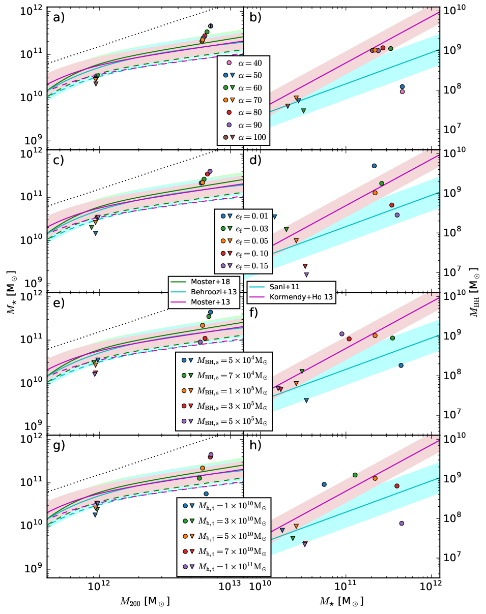
For the galaxy g7.92e12 the accretion parameter seems to have a threshold value of about . For the variation in stellar mass (Fig. 10a) does not show a clear trend but is possibly of stochastic nature. The black hole mass does not change significantly (Fig. 10b), demonstrating the self-regulating nature of black hole feedback. However, for the black hole feedback is insufficient to reduce the stellar mass to match the observed - relations (Fig. 10a) and the black hole mass rapidly drops below the observed - relations (Fig. 10b). For the galaxy g8.26e11 this threshold value seems to be smaller, possibly due to a higher resolution, as all simulations only show small variations in the - and - relations that are possibly of stochastic nature. Thus an accretion parameter of seems to be a reasonable choice.
6.2 Feedback efficiency
A higher feedback efficiency quenches the accretion of gas by the black hole, and thus leads to a lower black hole mass (Fig. 10d). The total amount of feedback energy injected into the gas for the galaxy g7.92e12 is for the values , i.e. even changing the feedback efficiency by a factor of 15 changes the total feedback energy by less than 20 per cent. Thus a higher feedback efficiency is compensated by a lower black hole mass, leading to approximately the same total feedback energy, again demonstrating the self-regulating nature of black hole feedback. The stellar mass is slightly decreasing with decreasing feedback efficiency (Fig. 10c), but this effect is small and could also be of stochastic nature. Feedback efficiencies of 0.10 and 0.15 far overpredict the - relation for the galaxy g7.92e12 (Fig. 10c), and feedback efficiencies of 0.01 and 0.03 far underpredict the - relation for the galaxy g8.26e11 (Fig. 10d), making a feedback efficiency of an optimal choice.
6.3 Black hole seed mass
Small seed masses of and provide insufficient feedback, leading the galaxy g7.92e12 to highly exceed the observed - relations (Fig. 10e). High seed masses of and bring the galaxy g7.92e12 to the edges of the observed - and - relations (Fig. 10e,f), leaving a seed mass of as optimal choice.
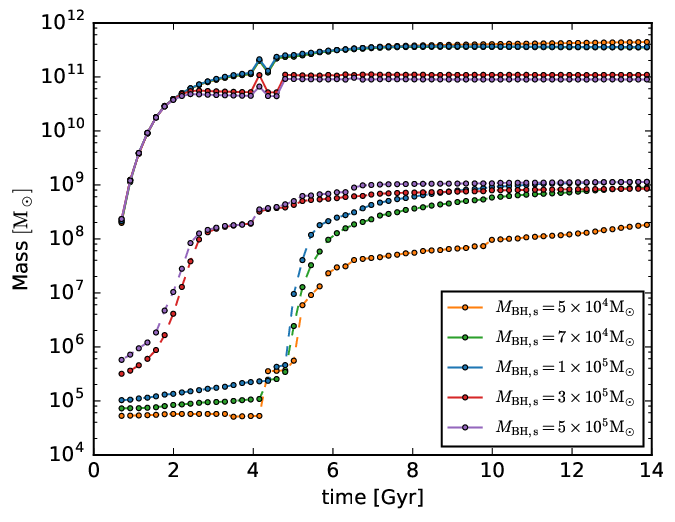
According to Fig. 10e,f the final black hole mass does not depend on the black hole seed mass (except for the lowest seed mass), but the final stellar mass does. This can be explained with Fig. 11, which shows the black hole mass and the stellar mass as a function of time for the galaxy g7.92e12 and for different black hole seed masses. The three lowest black hole seed masses show a black hole mass evolution as outlined in section 5: The growth rate is low at first, then black hole mergers trigger ‘runaway growth’ that is then stopped by feedback and ultimately leads to black hole masses in accordance with observations.
The two highest black hole seed masses show an entirely different evolution: Black hole mergers are not needed, the seed mass is already sufficiently high to trigger ‘runaway growth’.
Although the evolution of the black hole masses in both scenarios is entirely different at early times, they produce the same final black hole masses (except for the lowest seed mass), which can be attributed to the self-regulating nature of black hole feedback: Large black holes exert high feedback and allow for a low accretion rate, small black holes exert low feedback and allow for a high accretion rate.
Fig. 11 also shows the stellar mass as a function of time for different initial black hole seed masses. Until 2.5 gigayears the stellar masses evolve almost identical, then they start diverging: The higher the black hole seed mass the earlier the black hole accretion rate peaks, thus star formation is quenched earlier, which sets the stellar masses to ever lower values. The sudden jumps in the stellar mass at about 4-5 gigayears are caused by a merger event.
Different black hole seed masses lead to the same black hole mass, but to different stellar masses at redshift zero. However, calibration on scaling relations can be used to determine the optimal choice for the black hole seed mass.
6.4 Halo threshold mass
High halo threshold masses of or overpredict the - relation (Fig. 10g) for the galaxy g7.92e12, whereas decreasing the halo threshold mass to or moves the galaxy to the edge of the observed - relations (Fig. 10h). Thus a halo threshold mass of is the most reasonable choice.
The results in Fig. 10g,h resemble the results in Fig. 10e,f: Increasing the halo threshold mass is equivalent to reducing the black hole seed mass, thus the same ratio of halo threshold mass to black hole seed mass produces the same results. This can be explained as follows: The halo threshold mass basically determines the time the black hole is seeded. If with our standard parameters a black hole with is seeded at time t, increasing the halo threshold mass means the black hole with is seeded at a time t+dt, and reducing the black hole seed mass means a black hole with is seeded at time t. The former is equivalent to the latter, as the black hole with seeded at time t will have grown to at the time t+dt.
7 Summary
We introduce and test algorithms for black hole formation, accretion and feedback to the NIHAO project. For black hole formation we place a black hole in the centre of a halo once it exceeds a threshold mass, for black hole accretion we use the Bondi-Hoyle-Lyttleton parametrization, and for black hole feedback we deposit thermal energy, which is proportional to the black hole accretion rate, into the gas that surrounds the black hole. This addition to the NIHAO project allows us to extend the NIHAO suite of galaxies to higher masses.
Our galaxies show good agreement with the observed - and - relations that we use to calibrate the free parameters of our model. We also investigate the scatter of these relations and their time evolution. The scatter of both relations is decreasing with time for (higher redshifts possibly suffer from low number statistics and seeding effects), and is also lower than the observed scatter, possibly because we measure the intrinsic scatter of these relations without any observational uncertainties.
In the high mass, elliptical galaxies the quenching of star formation occurs after an increase of the black hole accretion rate, confirming that star formation is quenched by the black hole feedback. A parameter study confirms that we have chosen the optimal parameters within the framework of our model. Our simulations provide a valuable tool to study the effect of black hole feedback on galaxy formation and evolution.
Acknowledgements
The authors gratefully acknowledge the Gauss Centre for Supercomputing e.V. (www.gauss-centre.eu) for funding this project by providing computing time on the GCS Supercomputer SuperMUC at Leibniz Supercomputing Centre (www.lrz.de). A part of this research was carried out on the High Performance Computing resources at New York University Abu Dhabi. We used the software package pynbody Pontzen et al. 2013 for our analyses. AO is funded by the Deutsche Forschungsgemeinschaft (DFG, German Research Foundation) - MO 2979/1-1. We thank Tobias Buck for supplying the initial conditions for g7.92e12, g1.05e13 and g1.44e13.
References
- Anglés-Alcázar et al. (2017) Anglés-Alcázar D., Faucher-Giguère C.-A., Quataert E., Hopkins P. F., Feldmann R., Torrey P., Wetzel A., Kereš D., 2017, MNRAS, 472, L109
- Bate et al. (1995) Bate M. R., Bonnell I. A., Price N. M., 1995, MNRAS, 277, 362
- Behroozi et al. (2013) Behroozi P. S., Wechsler R. H., Conroy C., 2013, ApJ, 770, 57
- Bondi (1952) Bondi H., 1952, MNRAS, 112, 195
- Bondi & Hoyle (1944) Bondi H., Hoyle F., 1944, MNRAS, 104, 273
- Booth & Schaye (2009) Booth C. M., Schaye J., 2009, MNRAS, 398, 53
- Booth & Schaye (2010) Booth C. M., Schaye J., 2010, MNRAS, 405, L1
- Chabrier (2003) Chabrier G., 2003, PASP, 115, 763
- Choi et al. (2012) Choi E., Ostriker J. P., Naab T., Johansson P. H., 2012, ApJ, 754, 125
- Colberg & Di Matteo (2008) Colberg J. M., Di Matteo T., 2008, MNRAS, 387, 1163
- Conroy & van Dokkum (2012) Conroy C., van Dokkum P. G., 2012, ApJ, 760, 71
- Croft et al. (2009) Croft R. A. C., Di Matteo T., Springel V., Hernquist L., 2009, MNRAS, 400, 43
- Croton et al. (2006) Croton D. J., et al., 2006, MNRAS, 365, 11
- Debuhr et al. (2011) Debuhr J., Quataert E., Ma C.-P., 2011, MNRAS, 412, 1341
- Debuhr et al. (2012) Debuhr J., Quataert E., Ma C.-P., 2012, MNRAS, 420, 2221
- Di Matteo et al. (2005) Di Matteo T., Springel V., Hernquist L., 2005, Nature, 433, 604
- Di Matteo et al. (2008) Di Matteo T., Colberg J., Springel V., Hernquist L., Sijacki D., 2008, ApJ, 676, 33
- Dolag et al. (2016) Dolag K., Komatsu E., Sunyaev R., 2016, MNRAS, 463, 1797
- Dubois et al. (2015) Dubois Y., Volonteri M., Silk J., Devriendt J., Slyz A., Teyssier R., 2015, MNRAS, 452, 1502
- Dutton & Macciò (2014) Dutton A. A., Macciò A. V., 2014, MNRAS, 441, 3359
- Dutton et al. (2013a) Dutton A. A., et al., 2013a, MNRAS, 428, 3183
- Dutton et al. (2013b) Dutton A. A., Macciò A. V., Mendel J. T., Simard L., 2013b, MNRAS, 432, 2496
- Dutton et al. (2015) Dutton A. A., Macciò A. V., Stinson G. S., Gutcke T. A., Penzo C., Buck T., 2015, MNRAS, 453, 2447
- Dutton et al. (2017) Dutton A. A., et al., 2017, MNRAS, 467, 4937
- Eddington (1921) Eddington A. S., 1921, Z. Phys., 7, 351
- Ferrarese & Merritt (2000) Ferrarese L., Merritt D., 2000, ApJ, 539, L9
- Gebhardt et al. (2000) Gebhardt K., et al., 2000, ApJ, 539, L13
- Genel et al. (2014) Genel S., et al., 2014, MNRAS, 445, 175
- Gill et al. (2004) Gill S. P. D., Knebe A., Gibson B. K., 2004, MNRAS, 351, 399
- Grand et al. (2016) Grand R. J. J., Springel V., Gómez F. A., Marinacci F., Pakmor R., Campbell D. J. R., Jenkins A., 2016, MNRAS, 459, 199
- Haardt & Madau (2012) Haardt F., Madau P., 2012, ApJ, 746, 125
- Häring & Rix (2004) Häring N., Rix H.-W., 2004, ApJ, 604, L89
- Hirschmann et al. (2014) Hirschmann M., Dolag K., Saro A., Bachmann L., Borgani S., Burkert A., 2014, MNRAS, 442, 2304
- Hopkins & Quataert (2011) Hopkins P. F., Quataert E., 2011, MNRAS, 415, 1027
- Hopkins et al. (2014) Hopkins P. F., Kereš D., Oñorbe J., Faucher-Giguère C.-A., Quataert E., Murray N., Bullock J. S., 2014, MNRAS, 445, 581
- Hoyle & Lyttleton (1939) Hoyle F., Lyttleton R. A., 1939, Proceedings of the Cambridge Philosophical Society, 35, 405
- Jahnke & Macciò (2011) Jahnke K., Macciò A. V., 2011, ApJ, 734, 92
- Johansson et al. (2009) Johansson P. H., Naab T., Burkert A., 2009, ApJ, 690, 802
- Keller et al. (2014) Keller B. W., Wadsley J., Benincasa S. M., Couchman H. M. P., 2014, MNRAS, 442, 3013
- Khandai et al. (2015) Khandai N., Di Matteo T., Croft R., Wilkins S., Feng Y., Tucker E., DeGraf C., Liu M.-S., 2015, MNRAS, 450, 1349
- Knollmann & Knebe (2009) Knollmann S. R., Knebe A., 2009, ApJS, 182, 608
- Kormendy & Ho (2013) Kormendy J., Ho L. C., 2013, ARA&A, 51, 511
- Kormendy & Richstone (1995) Kormendy J., Richstone D., 1995, ARA&A, 33, 581
- Macciò et al. (2016) Macciò A. V., Udrescu S. M., Dutton A. A., Obreja A., Wang L., Stinson G. R., Kang X., 2016, MNRAS, 463, L69
- Magorrian et al. (1998) Magorrian J., et al., 1998, AJ, 115, 2285
- Matthee et al. (2017) Matthee J., Schaye J., Crain R. A., Schaller M., Bower R., Theuns T., 2017, MNRAS, 465, 2381
- Moster et al. (2013) Moster B. P., Naab T., White S. D. M., 2013, MNRAS, 428, 3121
- Moster et al. (2018) Moster B. P., Naab T., White S. D. M., 2018, MNRAS, 477, 1822
- Munshi et al. (2013) Munshi F., et al., 2013, ApJ, 766, 56
- Pillepich et al. (2018) Pillepich A., et al., 2018, MNRAS, 473, 4077
- Planck Collaboration et al. (2014) Planck Collaboration et al., 2014, A&A, 571, A16
- Pontzen et al. (2013) Pontzen A., Roškar R., Stinson G. S., Woods R., Reed D. M., Coles J., Quinn T. R., 2013, pynbody: Astrophysics Simulation Analysis for Python
- Rosas-Guevara et al. (2015) Rosas-Guevara Y. M., et al., 2015, MNRAS, 454, 1038
- Salpeter (1964) Salpeter E. E., 1964, ApJ, 140, 796
- Sani et al. (2011) Sani E., Marconi A., Hunt L. K., Risaliti G., 2011, MNRAS, 413, 1479
- Santos-Santos et al. (2018) Santos-Santos I. M., Di Cintio A., Brook C. B., Macciò A., Dutton A., Domínguez-Tenreiro R., 2018, MNRAS, 473, 4392
- Schaye et al. (2010) Schaye J., et al., 2010, MNRAS, 402, 1536
- Schaye et al. (2015) Schaye J., et al., 2015, MNRAS, 446, 521
- Shakura & Sunyaev (1973) Shakura N. I., Sunyaev R. A., 1973, A&A, 24, 337
- Shen et al. (2010) Shen S., Wadsley J., Stinson G., 2010, MNRAS, 407, 1581
- Sijacki et al. (2007) Sijacki D., Springel V., Di Matteo T., Hernquist L., 2007, MNRAS, 380, 877
- Sijacki et al. (2015) Sijacki D., Vogelsberger M., Genel S., Springel V., Torrey P., Snyder G. F., Nelson D., Hernquist L., 2015, MNRAS, 452, 575
- Springel et al. (2005) Springel V., Di Matteo T., Hernquist L., 2005, MNRAS, 361, 776
- Stinson et al. (2006) Stinson G., Seth A., Katz N., Wadsley J., Governato F., Quinn T., 2006, MNRAS, 373, 1074
- Stinson et al. (2013) Stinson G. S., Brook C., Macciò A. V., Wadsley J., Quinn T. R., Couchman H. M. P., 2013, MNRAS, 428, 129
- Tremmel et al. (2015) Tremmel M., Governato F., Volonteri M., Quinn T. R., 2015, MNRAS, 451, 1868
- Tremmel et al. (2017) Tremmel M., Karcher M., Governato F., Volonteri M., Quinn T. R., Pontzen A., Anderson L., Bellovary J., 2017, MNRAS, 470, 1121
- Vogelsberger et al. (2014) Vogelsberger M., et al., 2014, MNRAS, 444, 1518
- Wadsley et al. (2004) Wadsley J. W., Stadel J., Quinn T., 2004, New Astron., 9, 137
- Wadsley et al. (2017) Wadsley J. W., Keller B. W., Quinn T. R., 2017, MNRAS, 471, 2357
- Wang et al. (2015) Wang L., Dutton A. A., Stinson G. S., Macciò A. V., Penzo C., Kang X., Keller B. W., Wadsley J., 2015, MNRAS, 454, 83
- Wechsler & Tinker (2018) Wechsler R. H., Tinker J. L., 2018, ARA&A, 56, 435
- Weinberger et al. (2018) Weinberger R., et al., 2018, MNRAS, 479, 4056
- Wurster & Thacker (2013) Wurster J., Thacker R. J., 2013, MNRAS, 431, 2513
| galaxy | ||||||
| g7.55e11 | 932961 | 431968 | 327418 | 11.92 | 10.31 | 7.41 |
| g8.26e11 | 1070666 | 496667 | 424753 | 11.97 | 10.42 | 7.80 |
| g1.12e12 | 1062175 | 516394 | 430205 | 11.98 | 10.42 | 7.78 |
| g1.92e12 | 1960845 | 1035887 | 736102 | 12.28 | 10.66 | 8.25 |
| g2.79e12 | 3383907 | 1663073 | 1395558 | 12.49 | 10.93 | 8.39 |
| g7.55e11 | 1185149 | 455930 | 483752 | 11.95 | 10.49 | - |
| g8.26e11 | 1513265 | 518236 | 739749 | 12.01 | 10.67 | - |
| g1.12e12 | 1977112 | 564785 | 1222359 | 12.05 | 10.90 | - |
| g1.92e12 | 4018048 | 1200667 | 2467821 | 12.37 | 11.20 | - |
| g2.79e12 | 5598386 | 1800095 | 3099962 | 12.55 | 11.29 | - |
| g1.26e12 | 1253780 | 563159 | 462669 | 12.03 | 10.46 | 7.55 |
| g1.27e12 | 1150753 | 471966 | 605247 | 11.94 | 10.57 | 7.84 |
| g1.55e12 | 1469159 | 600775 | 679269 | 12.06 | 10.61 | 7.86 |
| g1.62e12 | 1063633 | 533023 | 327877 | 12.00 | 10.31 | 7.61 |
| g2.37e12 | 2159202 | 1098881 | 881920 | 12.30 | 10.73 | 8.30 |
| g2.71e12 | 2164500 | 1195318 | 596766 | 12.35 | 10.55 | 8.19 |
| g3.74e12 | 3397933 | 1715201 | 1182008 | 12.51 | 10.83 | 8.47 |
| g4.41e12 | 463537 | 250487 | 204647 | 12.55 | 10.83 | 8.84 |
| g4.55e12 | 503192 | 270807 | 164411 | 12.60 | 10.88 | 8.69 |
| g4.81e12 | 594745 | 306880 | 211336 | 12.66 | 11.01 | 8.70 |
| g4.84e12 | 523621 | 267346 | 185147 | 12.60 | 10.93 | 8.66 |
| g5.22e12 | 592556 | 313138 | 187130 | 12.67 | 10.96 | 8.58 |
| g5.41e12 | 644421 | 290846 | 352249 | 12.62 | 11.23 | 9.14 |
| g5.53e12 | 547812 | 306764 | 183274 | 12.65 | 10.83 | 8.69 |
| g6.53e12 | 591850 | 276231 | 266355 | 12.61 | 11.10 | 8.73 |
| g6.57e12 | 763439 | 356974 | 303556 | 12.73 | 11.15 | 8.75 |
| g6.86e12 | 838063 | 430471 | 303160 | 12.80 | 11.03 | 8.90 |
| g6.70e12 | 1290678 | 431794 | 693967 | 12.83 | 11.54 | 8.83 |
| g7.50e12 | 648889 | 387253 | 259728 | 12.74 | 11.08 | 9.32 |
| g7.55e12 | 860302 | 433196 | 262410 | 12.81 | 10.95 | 8.79 |
| g7.71e12 | 823620 | 415601 | 312032 | 12.79 | 11.17 | 8.94 |
| g7.92e12 | 1323285 | 446337 | 731566 | 12.84 | 11.55 | 9.06 |
| g8.08e12 | 1003594 | 486702 | 364796 | 12.86 | 11.22 | 9.00 |
| g8.45e12 | 779820 | 368069 | 308291 | 12.74 | 11.17 | 8.80 |
| g1.05e13 | 1146928 | 573974 | 489758 | 12.92 | 11.34 | 9.18 |
| g1.14e13 | 1354041 | 646068 | 532474 | 12.98 | 11.41 | 9.16 |
| g1.17e13 | 2085075 | 889400 | 782176 | 13.14 | 11.32 | 8.92 |
| g1.25e13 | 1217182 | 673068 | 367429 | 13.00 | 11.18 | 9.18 |
| g1.33e13 | 1918776 | 809672 | 751999 | 13.09 | 11.58 | 9.24 |
| g1.44e13 | 2836084 | 876310 | 1474963 | 13.14 | 11.86 | 8.94 |
| g1.54e13 | 1456656 | 722348 | 500173 | 13.03 | 11.36 | 9.17 |
| g1.57e13 | 889955 | 436443 | 310259 | 12.81 | 11.16 | 8.85 |
| g1.63e13 | 2089314 | 953300 | 684168 | 13.16 | 11.43 | 9.25 |
| g1.87e13 | 2278215 | 1101553 | 636663 | 13.23 | 11.39 | 9.29 |
| g2.02e13 | 1947099 | 1056092 | 840843 | 13.18 | 11.59 | 9.59 |
| g2.07e13 | 3177787 | 1497578 | 1020594 | 13.36 | 11.47 | 9.45 |
| g2.10e13 | 2972176 | 1249734 | 1072224 | 13.29 | 11.68 | 9.33 |
| g2.11e13 | 2434943 | 1250655 | 955862 | 13.26 | 11.63 | 9.45 |
| g2.20e13 | 1437878 | 847511 | 578127 | 13.08 | 11.41 | 9.46 |
| g2.37e13 | 2872994 | 1497621 | 1030754 | 13.34 | 11.59 | 9.54 |
| g2.58e13 | 3951084 | 1782390 | 1347000 | 13.44 | 11.66 | 9.47 |
| g3.26e13 | 4333704 | 2100752 | 1118595 | 13.51 | 11.45 | 9.52 |
| g3.42e12 | 2620934 | 1068134 | 1313357 | 12.30 | 10.91 | 8.12 |
| g3.78e13 | 3462973 | 1607283 | 1074439 | 13.39 | 11.51 | 9.45 |
| g3.89e13 | 5426667 | 2281160 | 1751607 | 13.55 | 11.81 | 9.70 |
| g5.41e12 | 1265524 | 337582 | 778618 | 12.73 | 11.59 | - |
| g6.86e12 | 1656812 | 453120 | 975692 | 12.86 | 11.69 | - |
| g7.50e12 | 1478432 | 443431 | 834490 | 12.85 | 11.62 | - |
| g7.92e12 | 1546499 | 455160 | 925496 | 12.85 | 11.65 | - |
| g1.05e13 | 2286298 | 658752 | 1301680 | 13.02 | 11.75 | - |
| g1.44e13 | 2738604 | 878724 | 1374316 | 13.14 | 11.83 | - |