Gradient Flow Finite Element Discretizations with Energy-Based Adaptivity for the Gross-Pitaevskii EquationThanks: The authors acknowledge the financial support of the Swiss National Science Foundation (SNF), Grant No. 200021 182524

An overview of models and numerical schemes for the GPE is provided in [7]. In general terms, the minimizer of the Gross–Pitaevskii energy functional (1) can be found either

1. (i)

   by solving the corresponding Euler-Lagrange formulation, i.e. the GPE,

2. (ii)

   or by direct minimization (under the normalization constraint (2)).

In the context of (i), classical spatial discretization approaches such as finite element methods [15, 33, 47, 46], finite difference schemes [22, 46], Fourier methods [12, 20], or (pseudo-) spectral methods [14, 10, 13] can be applied in a classical way. One possibility to deal with the nonlinearity occurring in the eigenvalue problem is to employ the Roothaan iteration scheme [21], also referred to as self-consistent field (SCF) iteration procedure. Alternatively, Newton’s method [18] or adaptations to the inverse power method [39] can be used. The idea of combining the iterative solution of the nonlinear eigenvalue problem and of mesh refinements in finite element discretizations has been addressed in [21, 19, 33, 22].

Among the class of methods (ii) we point to the imaginary time method [12, 4, 3, 8] which, upon employing an imaginary time transformation, $t\to-\imath t$, is based on the observation that the time-dependent GPE relaxes to the ground state as time evolves. In addition, upon interpreting the imaginary time method as a steepest descent method for the energy functional $\mathsf{E}$ from (1), the closely related gradient flow approaches [9, 11, 48, 36, 10, 25, 40, 46] can be derived. Further numerical solution methods in the scope of (ii) include a recently proposed preconditioned conjugate gradient method [5], direct energy minimization using symmetric properties [15] (which simplify the constraint minimization problem), or the combination of gradient flows and Riemannian optimization [26].

The aim of this work is to provide a numerical approximation procedure for the ground state of the Gross–Pitaevskii functional (1), under the constraint (2), which is based on a simultaneous interplay of gradient flow iterations and local adaptive finite element mesh refinements. This idea follows the recent developments on the (adaptive) iterative linearized Galerkin (ILG) methodology [34, 35, 23, 1, 2, 38], whereby adaptive discretizations and iterative nonlinearity solvers are combined in an intertwined way; we also refer to the closely related works [30, 29, 16, 32].

A key building block of the numerical scheme to be presented in this paper concerns the decision of whether local mesh refinements or gradient flow iterations should be given preference on a given finite element discretization space. This is accomplished by monitoring the energy decay resulting from the gradient flow, and by performing a comparison to the energy loss caused by the latest mesh refinement. Then, depending on which effect is currently dominant, we either undertake another gradient flow step, or the mesh is refined adaptively. We emphasize that this is a very natural approach for the given problem since both the (conforming) finite element method and the recently proposed gradient flow method [36] are both guaranteed to be energy-decreasing (owing to the variational principle). The proposed numerical method thereby generates a sequence of finite element approximations defined on adaptively refined spaces which provide a corresponding sequence of monotonically decreasing energies.

Proceeding along the energy minimization approach in [37], the adaptive mesh-refinement strategy in this work is based on identifying a subset of elements in the mesh for which a local refinement will potentially provide a significant (local) contribution to the total energy decay. To this end, for each element in the mesh, we first apply a local gradient flow step on a locally refined patch; these computations, since local and independent, can be done in parallel and only involve very few degrees of freedom. Then, a Dörfler marking strategy [27, Sec. 4.2] selects the most promising elements for refinement. The numerical tests illustrate optimal convergence rates in the number of unknowns for a variety of examples—both linear or nonlinear models, with smooth or irregular potentials, will be investigated.

In Section 2 we present the framework of the Gross-Pitaevskii equation and motivate its associated gradient flow system. Moreover, Section 3 is devoted to the finite element discretization and the adaptive mesh refinement strategy. Furthermore, Section 4 presents various numerical tests in 2D. Finally, we add some concluding remarks in Section 5.

We observe that the energy functional $\mathsf{E}$ from (1) is Fréchet differentiable on the Sobolev space $\mathbb{H}:=\mathrm{H}^{1}_{0}(\Omega)$ (defined to be the space of all functions with weak gradient in $\mathrm{L}^{2}(\Omega)^{d}$ and zero trace along the boundary $\partial\Omega$); indeed, a simple calculation reveals that

where $\langle\cdot,\cdot\rangle$ signifies the dual product in $\mathbb{H}^{\star}\times\mathbb{H}$. The Euler-Lagrange formulation of the constrained minimization problem

with $S_{\mathbb{H}}:=\{v\in\mathbb{H}:\|v\|_{{\rm L}^{2}(\Omega)}=1\}$ signifying the $\mathrm{L}^{2}(\Omega)$-unit sphere in $\mathbb{H}$, is given by

Here, the scalar $\lambda$ takes the role of a Lagrange multiplier corresponding to the norm constraint (2). The nonlinear eigenvalue problem (4) is called the Gross–Pitaevskii equation (GPE). If $v\in S_{\mathbb{H}}$ is an eigenfunction of (4) associated with an eigenvalue $\lambda$, then we note that

Given that $V\geq 0$ (almost everywhere in $\Omega$) and $\beta\geq 0$, the Gross–Pitaevskii eigenvalue problem (4) has a unique ($\mathrm{L}^{2}(\Omega)$-normalized) positive eigenfunction $u_{\mathrm{GS}}>0$ which is the ground state of the Bose–Einstein condensate (1), see [36, Lem. 5.4]; in particular, $u_{\mathrm{GS}}$ is an eigenfunction to the minimal (and simple) eigenvalue, signified by $\lambda_{\mathrm{GS}}$ of (4), see [20].

The ground state $u_{\mathrm{GS}}$ will be determined iteratively. To this end, we employ the projected gradient flow approach proposed in [36]. One of the key ideas is to introduce a weighted energy inner product on $\mathbb{H}\times\mathbb{H}$: For fixed $z\in\mathbb{H}$, we let

Owing to the Riesz representation theorem, for any $v\in\mathbb{H}$, it exists a unique $\mathsf{G}_{z}(v)\in\mathbb{H}$ such that

If $z\neq 0$, we notice that $a_{z}(\mathsf{G}_{z}(z),z)=\|z\|^{2}_{\mathrm{L}^{2}(\Omega)}>0$, and therefore $\mathsf{G}_{z}(z)\neq 0$. Hence, we may consider the linear mapping

where

for $z=0$, we have $\mathbb{T}_{0}=\mathbb{H}$, and $\mathsf{P}_{0}$ is the identity map. Using (7), it is fairly elementary to verify that

i.e. $\mathsf{P}_{z}$ is the orthogonal projection onto the (tangential plane) $\mathbb{T}_{z}$ with respect to the $a_{z}$-inner product.

Based on the above definitions, we are now ready to present the gradient flow induced by the inner product from (6). More precisely, we consider a trajectory $u:\,[0,\infty)\to\mathbb{H}$ which, for a given initial value $u(0)=u_{0}\in S_{\mathbb{H}}$, follows the dynamical system

The existence of a solution $u$ has been discussed in [36, Sec. 3.1 & 3.2].

In order to motivate the gradient flow system (10), we briefly revisit some arguments from [36, Proof of Theorem 3.2]:

1. (i)

   For any $v,z\in\mathbb{H}$, we define $\nabla_{z}\mathsf{E}(v)\in\mathbb{H}$ to be the Riesz representative of the steepest descend direction $\mathsf{E}^{\prime}(v)$ at $v$ with respect to the $a_{z}$-inner product, i.e.

   $$a_{z}(\nabla_{z}\mathsf{E}(v),w)=\langle\mathsf{E}^{\prime}(v),w\rangle\qquad\forall w\in\mathbb{H}.$$

   Then, using (10), employing (9) respectively (6), and recalling (3), for any $t>0$, we notice that

   	$\displaystyle a_{u(t)}(\dot{u}(t),w)$	$\displaystyle=a_{u(t)}(-\mathsf{P}_{u(t)}(u(t)),w)$
   		$\displaystyle=a_{u(t)}(-u(t),\mathsf{P}_{u(t)}(w))$
   		$\displaystyle=\langle-\mathsf{E}^{\prime}(u(t)),\mathsf{P}_{u(t)}(w)\rangle$
   		$\displaystyle=a_{u(t)}(-\nabla_{u(t)}\mathsf{E}(u(t)),\mathsf{P}_{u(t)}(w))$
   		$\displaystyle=a_{u(t)}(\mathsf{P}_{u(t)}(-\nabla_{u(t)}\mathsf{E}(u(t))),w),$

   for any $w\in\mathbb{H}$. This implies that the gradient flow from (10) follows the orthogonal projection of the steepest descend direction $-\nabla_{u(t)}\mathsf{E}(u(t))$, for $t>0$, onto the tangential plane $\mathbb{T}_{u(t)}$.

2. (ii)

   Observe that

   $$\dot{u}(t)\in\mathbb{T}_{u(t)}\qquad\forall t>0.$$

   (11)

   Hence,

   $\displaystyle\frac{\mathsf{d}}{\mathsf{dt}}\left\|u(t)\right\|_{\mathrm{L}^{2}(\Omega)}^{2}=2(u(t),\dot{u}(t))_{\mathrm{L}^{2}(\Omega)}=0\qquad\forall t>0.$

   In particular, it follows that $\left\|u(t)\right\|_{\mathrm{L}^{2}(\Omega)}=\left\|u(0)\right\|_{\mathrm{L}^{2}(\Omega)}=1$. This means that the gradient flow stays on the sphere $S_{\mathbb{H}}$ for any $t>0$, i.e., physically speaking, it is mass preserving; cf. [36, Lem. 3.3].

3. (iii)

   Using again (11) and invoking (9), for any $t>0$, it holds that

   $$\frac{\mathsf{d}}{\mathsf{dt}}\mathsf{E}(u(t))=\langle\mathsf{E}^{\prime}(u(t)),\dot{u}(t)\rangle=a_{u(t)}(u(t),\dot{u}(t))=-a_{u(t)}(-\mathsf{P}_{u(t)}(u(t)),\dot{u}(t)).$$

   (12)

   Thus, implementing (10) yields

   $$\langle\mathsf{E}^{\prime}(u(t)),\dot{u}(t)\rangle=-a_{u(t)}(\dot{u}(t),\dot{u}(t))\leq 0\qquad\forall t>0,$$

   i.e. the energy $\mathsf{E}(t)$ is monotone decreasing as $t\to\infty$; cf. [36, Lem. 3.3].

4. (iv)

   Since $\mathsf{E}(v)$ is nonnegative for any $v\in\mathbb{H}$, the monotonicity property from (iii) implies that there is $\mathsf{E}^{\star}\geq 0$ with $\lim_{t\to\infty}\mathsf{E}(u(t))=\mathsf{E}^{\star}<\infty$. Hence, applying (12), we obtain the identity

   $$0\leq\int_{0}^{\infty}a_{u(\tau)}(\dot{u}(\tau),\dot{u}(\tau))\,\mathsf{d}\tau=\mathsf{E}(u_{0})-\mathsf{E}^{\star}<\infty,$$

   which implies that $\int_{0}^{\infty}\|\nabla\dot{u}(\tau)\|^{2}_{\mathrm{L}^{2}(\Omega)}\,\mathsf{d}\tau$ is bounded. It follows that $u(t)$ has a limit $u^{\star}\in\mathbb{H}$ as $t\to\infty$ (with $\left\|u^{\star}\right\|_{{\rm L}^{2}(\Omega)}=1$, cf. (ii)), and $\mathsf{P}_{u^{\star}}(u^{\star})=0$ upon taking the limit in (10). Consequently, we deduce from (8) that $u^{\star}=\lambda^{\star}\mathsf{G}_{u^{\star}}(u^{\star})$, where

   $$\lambda^{\star}=\frac{\|u^{\star}\|^{2}_{\mathrm{L}^{2}(\Omega)}}{a_{u^{\star}}(\mathsf{G}_{u^{\star}}(u^{\star}),\mathsf{G}_{u^{\star}}(u^{\star}))}.$$

   Therefore, exploiting (7), for all $w\in\mathbb{H}$, we infer that

   $$\langle\mathsf{E}^{\prime}(u^{\star}),w\rangle=a_{u^{\star}}(u^{\star},w)=\lambda^{\star}a_{u^{\star}}(\mathsf{G}_{u^{\star}}(u^{\star}),w)=\lambda^{\star}(u^{\star},w)_{\mathrm{L}^{2}(\Omega)},$$

   (13)

   i.e. $u^{\star}\not\equiv 0$ is an eigenfunction for the GPE (4) to the eigenvalue $\lambda^{\star}$. We note that $u^{\star}$ can be any eigenfunction satisfying (13), respectively (4); in particular, it is not necessarily the ground state.

For the purpose of computing an approximation of the continuous gradient flow trajectory from (10), we use the forward Euler discretization method. For a given initial value $u^{0}\in S_{\mathbb{H}}$ this yields a sequence of functions $\{u^{n}\}_{n\geq 0}\subset S_{\mathbb{H}}$ which, for $n\geq 0$, is defined by

Here, $\{\tau_{n}\}_{n\geq 0}$ is a sequence of positive (discrete) time steps that is assumed uniformly bounded from above and below with bounds $\tau_{\max}$ and $\tau_{\min}$, respectively, such that $0<\tau_{\min}\leq\tau_{n}\leq\tau_{\max}<\infty$. The scheme (14) is called discrete gradient flow iteration (GFI).

Consider a sequence of conforming and shape-regular partitions $\{\mathcal{T}_{N}\}_{N\in\mathbb{N}}$ of the domain $\Omega$ into simplicial elements $\mathcal{T}_{N}=\{\kappa\}_{\kappa\in\mathcal{T}_{N}}$ (i.e. triangles for $d=2$ and tetrahedra for $d=3$). Moreover, for a (fixed) polynomial degree $p\in\mathbb{N}$ and any subset $\omega\subset\mathcal{T}_{N}$, we introduce the finite element space

with $\mathbb{P}_{p}(\kappa)$ signifying the (local) space of all polynomials of maximal total degree $p$ on $\kappa$, $\kappa\in\mathcal{T}_{N}$. Furthermore, similarly as before, we denote by

the $\mathrm{L}^{2}(\Omega)$-unit sphere in $\mathbb{V}(\omega)$. In the sequel, we apply the notations $\mathbb{X}_{N}:=\mathbb{V}(\mathcal{T}_{N})$ and $S_{N}:=S_{\mathbb{V}(\mathcal{T}_{N})}$. We further denote by $\mathsf{E}_{N}:=\mathsf{E}|_{\mathbb{X}_{N}}$ the restriction of the energy functional $\mathsf{E}$ from (1) to the Galerkin space $\mathbb{X}_{N}$. Then, due to the compactness of $S_{N}$, it exists a minimizer $u_{N}\in\mathbb{X}_{N}$ of $\mathsf{E}_{N}$, i.e. $\mathsf{E}(u_{N})=\min_{v\in S_{N}}\mathsf{E}(v)$, with $(u_{N},1)_{{\rm L}^{2}(\Omega)}\geq 0$. It is not known, however, if $u_{N}$ is unique (up to the sign), see, e.g., [20]. Furthermore, if $\{\mathbb{X}_{N}\}_{N\in\mathbb{N}}$ is a dense family of finite element subspaces of $\mathbb{H}$, then any sequence of minimizers $u_{N}\in S_{N}$ of $\mathsf{E}_{N}$ with $(u_{N},1)_{{\rm L}^{2}(\Omega)}\geq 0$ converges in $\mathrm{H}^{1}(\Omega)$ to the ground state $u_{\mathrm{GS}}$ of $\mathsf{E}$; we refer to [20, Theorem 1] or [50, Theorem 3.1].

Let us define the (space) discrete version of the gradient flow iteration (14) on a finite element subspace $\mathbb{X}_{N}\subset\mathbb{H}$. For $u\in\mathbb{X}_{N}$ we denote by $\mathsf{G}^{N}(u)\in\mathbb{X}_{N}$ the unique solution of

cf. (7). For given $u\in\mathbb{X}_{N}$, note that the computation of $\mathsf{G}^{N}(u)$ is a standard linear source problem; it can be solved by any linear solver at the disposal of the user. Then, for $n\geq 0$, the space discrete GFI is given by

with a sequence of discrete time steps $\{\tau_{N}^{n}\}_{n\geq 0}$ as in (14).

For any element $\kappa\in\mathcal{T}_{N}$ we consider the open patch $\omega_{\kappa}$ comprising of $\kappa$ and its immediate face-wise neighbours. Moreover, given $\kappa\in\mathcal{T}_{N}$, we define the modified patch $\widetilde{\omega}_{\kappa}$ by uniformly (red) refining the element $\kappa$ into a (fixed) number of subelements; here, we assume that the introduction of any hanging nodes in $\omega_{\kappa}$ is removed by doing (e.g. green) refinements, see Figure 1. We remark that the notions of red and green refinements refer to standard element subdivision techniques in automatic mesh adaptation; further details can be found, e.g., in [41, §4.10.2.2] (or [6], where red refinement is termed bisection-type mesh refinement).

We consider basis functions $\{\xi^{1}_{\kappa},\ldots,\xi^{m_{\kappa}}_{\kappa}\}$ of the locally supported space $\mathbb{V}(\widetilde{\omega}_{\kappa})$. Furthermore, for any given $v\in\mathbb{V}(\mathcal{T}_{N})$, we introduce the extended space

Suppose we have found an accurate approximation $u_{N}^{n}\in\mathbb{X}_{N}$ of the discrete GPE (17), for some $n\geq 0$. Then, by performing one local discrete GFI-step in $\widehat{\mathbb{V}}(\widetilde{\omega}_{\kappa};u_{N}^{n})\subset\mathbb{H}$ we obtain a new local approximation, denoted by $\widetilde{u}_{N,\kappa}^{n}\in\widehat{\mathbb{V}}(\widetilde{\omega}_{\kappa};u_{N}^{n})$, with $\left\|\widetilde{u}_{N,\kappa}^{n}\right\|_{\mathrm{L}^{2}(\Omega)}=1$. We emphasize that $\widehat{\mathbb{V}}(\widetilde{\omega}_{\kappa};u_{N}^{n})$ has a small dimension, and hence the discrete GFI (16) based on $\widehat{\mathbb{V}}(\widetilde{\omega}_{\kappa};u_{N}^{n})$ entails hardly any computational cost (for instance, for dimension $d=2$ and polynomial degree $p=1$, the dimension of the locally refined space $\widehat{\mathbb{V}}(\widetilde{\omega}_{\kappa};u_{N}^{n})$, cf. Figure 1, is typically 3 or 4).

By modus operandi of the discrete GFI (16), the above construction leads in general, see Remark 3.2, to the (local) energy decay

for all $\kappa\in\mathcal{T}_{N}$. The value $\Delta\mathsf{E}_{N}^{n}(\kappa)$ indicates the potential energy reduction due to a refinement of the element $\kappa$. This observation motivates the energy-based adaptive mesh refinement procedure outlined in Algorithm 1.

From a practical viewpoint, once the discrete GFI approximation from (16) is close to a solution of (17), on a given finite element space, we expect that any further GFI steps will no longer contribute an essential decay to the energy in (19). In this case, in order to further reduce the energy, we need to enrich the finite element space appropriately. More specifically, for $N\geq 1$, suppose that we have performed a reasonable number $n\geq 1$ (possibly depending on $N$) of GFI-iterations (16) in $\mathbb{X}_{N-1}$. Consider now a (hierarchically) refined mesh $\mathcal{T}_{N}$ of $\mathcal{T}_{N-1}$, for example, obtained by Algorithm 1. Then we may embed the final guess $u^{n}_{N-1}\in\mathbb{X}_{N-1}$ on the previous space into the enriched finite element space $\mathbb{X}_{N}$ in order to obtain an initial guess on the refined mesh $\mathcal{T}_{N}$:

For each GFI-iteration $n$ we monitor two quantities. Firstly, we introduce the increment on each iteration given by

Secondly, we compare $\mathrm{inc}_{N}^{n}$ to the energy loss as compared to the previous mesh refinement, i.e.

We stop the iteration for $n\geq 1$ as soon as $\mathrm{inc}_{N}^{n}$ becomes small compared to $\Delta\mathsf{E}_{N}^{n}$, i.e. once there is no notable benefit (relatively speaking) in performing any more discrete GFI steps on the current space $\mathbb{X}_{N}$. Specifically, for $n\geq 1$, this is expressed by the bound

for some parameter $0<\gamma<1$. We implement this procedure in Algorithm 2.

We comment on the computational cost of one loop occurring in Algorithm 2. This is essentially comprised of a number of GFI steps on a given Galerkin space $\mathbb{X}_{N}$, and on one adaptive (local) mesh refinement (using Algorithm 1).

• •

  The cost of one GF iteration is dominated by the computation of the Riesz-representative $\mathsf{G}^{N}(u_{N}^{n})$ from (15), and, thereby, depends primarily on the dimension $\textrm{dim}(\mathbb{X}_{N})$ of the finite element space $\mathbb{X}_{N}$. Specifically, the solution of (15) (for given $u^{n}_{N}$) amounts to a computational work that scales like $\mathcal{O}(\textrm{dim}(\mathbb{X}_{N})^{\alpha})$, with a parameter $\alpha\geq 1$ depending on the linear solver employed.

• •

  The local finite element space $\widehat{\mathbb{V}}(\widetilde{\omega}_{\kappa};u_{N}^{n})$ contains $m_{\kappa}$ local and one global basis function, namely $u_{N}^{n}$, which is the same for all elements $\kappa$. The mesh-refinement procedure contains one GF iteration as described in (16), however, on the local space $\widehat{\mathbb{V}}(\widetilde{\omega}_{\kappa};u_{N}^{n})$. This, in turn, requires the solution of a linear system involving $m_{\kappa}$ local and one global degrees of freedom. In particular, only one entry of the corresponding matrix requires a global integration, which can be computed element-by-element (and, therefore, in parallel); all other matrix entries are represented by local integrals. Finally, note that the entry requiring global integration is the same for all local GF iterations and all elements $\kappa$, and, thus, needs to be computed only once within each step of the loop in Algorithm 2.

  A similar observation holds for the computation of the local energy decays. In fact, for $u_{N}^{n}\in\mathbb{X}_{N}$, denoting, as in Algorithm 1, the locally improved approximation by $\widetilde{u}_{N,\kappa}^{n}$, we have the linear combination

  $$\widetilde{u}_{N,\kappa}^{n}=\mu u_{N}^{n}+\sum_{i=1}^{m_{\kappa}}\mu_{i}\xi_{\kappa}^{i},$$

  for suitable $\mu,\mu_{i}\in\mathbb{R}$, $i\in\{1,\dotsc,m_{\kappa}\}$. Then, it is elementary to verify that

  $$\mathsf{E}(\widetilde{u}_{N}^{n})=\mathsf{E}(\mu u_{N}^{n})-\mathsf{E}_{\widetilde{w}_{\kappa}}(\mu u_{N}^{n})+\mathsf{E}_{\widetilde{w}_{\kappa}}(\widetilde{u}_{N,\kappa}^{n}),$$

  where $\mathsf{E}_{\widetilde{\omega}_{\kappa}}(\cdot)$ represents the contribution from the elements comprising the patch $\widetilde{\omega}_{\kappa}$ to the total energy $\mathsf{E}(\cdot)$. We emphasize that the second and third terms on the right-hand side only require the computation of a local integral. Moreover, for the term $\mathsf{E}(\mu u_{N}^{n})$ we observe that $\mathsf{E}(\mu u_{N}^{n})=:\mu^{2}\mathsf{E}^{n}_{N,1}+\mu^{4}\mathsf{E}^{n}_{N,2},$ with

  $\displaystyle\mathsf{E}^{n}_{N,1}$

  $\displaystyle=\int_{\Omega}\left(\frac{1}{2}|\nabla u_{N}^{n}|^{2}+V(\bm{x})|u_{N}^{n}|^{2}\right)\,\mathsf{d}\bm{x},$

  $\displaystyle\mathsf{E}^{n}_{N,2}$

  $\displaystyle=\int_{\Omega}\frac{\beta}{2}|u_{N}^{n}|^{4}\,\mathsf{d}\bm{x}.$

  Thus, for each patch, the energy $\mathsf{E}(\mu u_{N}^{n})$ is a combination of the above two global integrals, which need to be computed once only, and can be split into elementwise contributions.

  Altogether, the computational cost for the local GF iterations and corresponding local energy decays therefore scales linearly with the number of elements in the mesh, i.e. with $\textrm{dim}(\mathbb{X}_{N})$, and can be performed fully in parallel. The same observation applies to the element marking and local mesh refinement procedure, which compares to the evaluation of standard residual based a posteriori error estimators.

In summary, we find that the computational work for one loop in Algorithm 2 scales with $\mathcal{O}(\textrm{dim}(\mathbb{X}_{N})^{\alpha})$, where $\alpha\geq 1$ depends on the global finite element solver. In particular, our scheme exhibits a similar complexity as standard adaptive finite element discretization procedures for linear problems (provided that the number of GFI steps remain reasonably modest).

We begin by testing our algorithm for the Laplace eigenvalue problem, which is to find $u\in\mathbb{H}=\mathrm{H}^{1}_{0}(\Omega)$ and $\lambda>0$ such that

here, $\Omega=(0,2)^{2}\setminus[1,2]\times[0,1]$ is an $L$-shaped domain. This problem is of interest since the eigenfunction to the lowest eigenvalue $\lambda_{1}$, i.e. the ground state, has a singularity at the re-entrant corner point $(1,1)$. From [31] it is known that $9.6397238\leq\lambda_{1}\leq 9.6397239$. Taking the lower bound (divided by 2, cf. (5) for $\beta=0$) as reference value, Figure 2 demonstrates the optimal convergence rate for the minimal energy approximation.

We consider the case where $\beta=0$ in (1), and $V(x,y)=\nicefrac{{1}}{{2}}(x^{2}+9y^{2})$ is a smooth function:

Note that the associated eigenvalue problem (4) is linear for this example. It is known that, for $\Omega=\mathbb{R}^{2}$, the energy of the ground state is given by $\mathsf{E}(u_{\mathrm{GS}})=2$, see, e.g., [7]. We note that the mass of $u_{\mathrm{GS}}$ is essentially concentrated in a vicinity of the origin $\bm{0}$ due to the global minimum of $V$ at $\bm{0}$. Therefore, the restriction to the bounded domain $\Omega:=(-10,10)^{2}\subset\mathbb{R}^{2}$, which we use in our computations, has almost no effect on the minimal value of the ground state energy. Figure 3 (left) illustrates that the approximation of the energy converges with optimal rate in terms of the numbers of degrees of freedom. In addition, we see that the mesh is mainly refined around the origin, where the mass of the ground state $u_{\mathrm{GS}}$ is concentrated, see Figure 3 (right). These results underline that the proposed adaptive gradient flow procedure effectively detects the local behaviour of the model.

We perform another experiment with $\beta=0$ in (1), i.e. the associated eigenvalue problem (4) is again linear. In contrast to the previous example, however, we consider a potential $V(\bm{x})=(2|\bm{x}|)^{-1}$ which features a severe point singularity at the origin $\bm{0}=(0,0)$. Specifically, the energy functional is given by

with $\Omega=\left(\nicefrac{{-1}}{{2}},\nicefrac{{1}}{{2}}\right)^{2}$. This experiment has been conducted already in [45], where the authors obtained an approximated minimal eigenvalue $\lambda_{\mathrm{GS}}=25.934923921168$ for the corresponding GPE (4); we compare our results to this reference value (divided by 2 on account of (5)). We can see from Figure 4 that the proposed Algorithm 2 achieves a sequence of energy approximations for the ground state which decays at an (almost) optimal rate.

We test a final example with $\beta=0$. The potential $V$ is given by the sum of four Gaussian bells, see Figure 5 (left). This experiment is borrowed from [44, Experiment 4.2], however, with a (constant) shift such that $V\geq 0$ in the underlying domain $\Omega=(0,2\pi)^{2}$. As we can see from Figure 5 (right), the mass of the ground state is mainly concentrated at two adjacent hills in the lower left part of the domain; we note that this is perfectly in line with the results obtained in the paper [44]. Moreover, the energy-based adaptive mesh refinement has properly resolved the two local hills featured in the ground state $u_{\mathrm{GS}}$, see Figure 6.

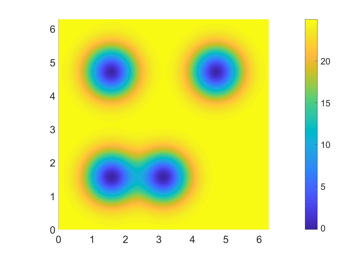
The authors from [44] have computed an approximated minimal eigenvalue $\lambda_{\mathrm{GS}}=16.6879$, whereby this is the value adapted for our reformulation of the problem. Based on this approximation, we observe an optimal rate of convergence for the energy of the ground state in Figure 7 (left). We remark, for this example, that the performance of Algorithm 2 crucially depends on the choice of the parameter $\gamma$ in Line 6. Indeed, if $\gamma=0.5$ (instead of $\gamma=0.1$) is selected, then the numerical results exhibit a considerably less favourable asymptotic convergence regime, see Figure 7 (right). An explanation can be inferred from Figure 8: We see that the choice $\gamma=0.1$ leads to a significantly higher number of gradient flow steps on each Galerkin space $\mathbb{X}_{N}$, which seems to be essential for the effective numerical solution of this problem.

We now consider a nonlinear Bose-Einstein condensate, i.e. $\beta=1000\gg 0$ in (1), and use the smooth potential $V(\bm{x})=\nicefrac{{1}}{{2}}|\bm{x}|^{2}$:

the domain is given by $\Omega=(-6,6)^{2}$. This experiment was conducted previously in [36], where an approximation $\mathsf{E}(u_{\mathrm{GS}})\approx 11.9860647$ for the energy of the ground state has been documented. Based on the adaptive Algorithm 2 presented in this work, a smaller value for the ground state energy has been computed; we suppose that this (improved) approximation results from the adaptive (and thereby more effective) refinement of the meshes. To be specific, we have obtained the approximation $\mathsf{E}(u_{\mathrm{GS}})\approx\underline{11.98605}121\dotsc$ based on an adaptively refined mesh with $\mathcal{O}(10^{7})$ degrees of freedom; here, the underlined digits are stable (i.e. the computations indicate that they do not change any more as the iterations continue). Using this as reference value, we obtain optimal convergence for the approximation of the energy of the ground state, see Figure 9.

In order to study the dependence of the computational work on the strength of the nonlinearity, we have performed the same experiment for different values of $\beta$. As can be seen from Table 4.5, our algorithm does not seem to be sensitive with respect this parameter. Indeed, after an initial phase, the number of GF iterations on a given mesh is independent of $\beta$. Moreover, for $\gamma=0.5$, this holds true already from the start, i.e. even for the initial mesh (not displayed here). We remark that analogous results have been observed recently in [49] for a multigrid method.

As before, we choose $\Omega=(-6,6)^{2}$ and $\beta=1000$, with an oscillating potential function $V$, see Figure 11 (left) for its contour plot. More precisely, the energy functional is given by

This experiment was also considered in [36] with an asserted approximation $\mathsf{E}(u_{\mathrm{GS}})\approx 30.40965$ of the ground state energy. Based on a sufficiently fine uniform initial mesh (with $128$ elements), our algorithm yields the approximation $\mathsf{E}(u_{\mathrm{GS}})\approx\underline{30.387}533\dotsc$ for $\mathcal{O}(10^{7})$ degrees of freedom. In Figure 10 (left) we have depicted the error for the approximations of the ground state energy with respect to our reference value. This plot indicates an asymptotically optimal rate of convergence of Algorithm 2 for the given problem.

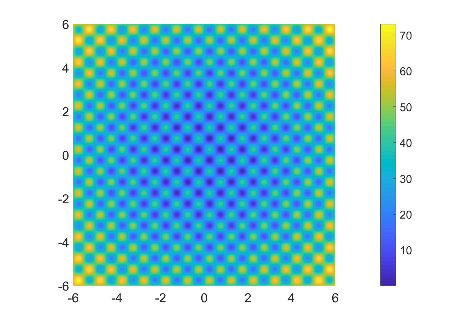
As in Example 4.4, we have also run this experiment for both values $\gamma=0.1$ and $\gamma=0.5$. In contrast to the previous test, we observe no considerable difference in the performance of the corresponding computations. Indeed, except for the first two meshes, the number of gradient flow steps on each Galerkin space is the same for both cases, see Figure 12.

Finally, we revisit the test problem [11, Example 4.3.II]:

References

- [1] M. Amrein and T. P. Wihler, An adaptive Newton-method based on a dynamical systems approach, Commun. Nonlinear Sci. Numer. Simul. 19 (2014), no. 9, 2958–2973.
- [2] by same author, Fully adaptive Newton-Galerkin methods for semilinear elliptic partial differential equations, SIAM J. Sci. Comput. 37 (2015), no. 4, A1637–A1657.
- [3] X. Antoine and R. Duboscq, GPELab, a Matlab toolbox to solve Gross–Pitaevskii equations I: Computation of stationary solutions, Computer Physics Communications 185 (2014), no. 11, 2969–2991.
- [4] by same author, Robust and efficient preconditioned Krylov spectral solvers for computing the ground states of fast rotating and strongly interacting Bose–Einstein condensates, Journal of Computational Physics 258 (2014), 509–523.
- [5] X. Antoine, A. Levitt, and Q. Tang, Efficient spectral computation of the stationary states of rotating Bose–Einstein condensates by preconditioned nonlinear conjugate gradient methods, Journal of Computational Physics 343 (2017), 92–109.
- [6] R. E. Bank, A. H. Sherman, and A. Weiser, Refinement algorithms and data structures for regular local mesh refinement, Scientific computing (Montreal, Que., 1982), IMACS Trans. Sci. Comput., I, IMACS, New Brunswick, NJ, 1983, pp. 3–17.
- [7] W. Bao, Mathematical models and numerical methods for Bose-Einstein condensation, Proceedings of the International Congress of Mathematicians—Seoul 2014. Vol. IV, Kyung Moon Sa, Seoul, 2014, pp. 971–996.
- [8] W. Bao and Y. Cai, Mathematical theory and numerical methods for Bose-Einstein condensation, Tech. Report 1212.5341, arxiv.org, 2012.
- [9] W. Bao, Y. Cai, and H. Wang, Efficient numerical methods for computing ground states and dynamics of dipolar Bose–Einstein condensates, Journal of Computational Physics 229 (2010), no. 20, 7874–7892.
- [10] W. Bao, I-L. Chern, and F.Y. Lim, Efficient and spectrally accurate numerical methods for computing ground and first excited states in Bose–Einstein condensates, Journal of Computational Physics 219 (2006), no. 2, 836–854.
- [11] W. Bao and Q. Du, Computing the ground state solution of Bose–Einstein condensates by a normalized gradient flow, SIAM Journal on Scientific Computing 25 (2004), no. 5, 1674–1697.
- [12] W. Bao, D. Jaksch, and P. Markowich, Numerical solution of the Gross–Pitaevskii equation for Bose–Einstein condensation, Journal of Computational Physics 187 (2003), no. 1, 318–342.
- [13] W. Bao, H. Li, and J. Shen, A generalized-Laguerre–Fourier–Hermite pseudospectral method for computing the dynamics of rotating Bose–Einstein condensates, SIAM Journal on Scientific Computing 31 (2009), no. 5, 3685–3711.
- [14] W. Bao and J. Shen, A Fourth-Order Time-Splitting Laguerre–Hermite Pseudospectral Method for Bose–Einstein Condensates, SIAM Journal on Scientific Computing 26 (2005), no. 6, 2010–2028.
- [15] W. Bao and W. Tang, Ground-state solution of Bose–Einstein condensate by directly minimizing the energy functional, Journal of Computational Physics 187 (2003), no. 1, 230–254.
- [16] C. Bernardi, J. Dakroub, G. Mansour, and T. Sayah, A posteriori analysis of iterative algorithms for a nonlinear problem, J. Sci. Comput. 65 (2015), no. 2, 672–697.
- [17] S.N. Bose, Plancks Gesetz und Lichtquantenhypothese, Zeitschrift für Physik 26 (1924), no. 1, 178–181.
- [18] M. Caliari, A. Ostermann, S. Rainer, and M. Thalhammer, A minimisation approach for computing the ground state of Gross–Pitaevskii systems, Journal of Computational Physics 228 (2009), no. 2, 349–360.
- [19] E. Cancès, R. Chakir, L. He, and Y. Maday, Two-grid methods for a class of nonlinear elliptic eigenvalue problems, IMA Journal of Numerical Analysis 38 (2017), no. 2, 605–645.
- [20] E. Cancès, R. Chakir, and Y. Maday, Numerical analysis of nonlinear eigenvalue problems, J. Sci. Comput. 45 (2010), no. 1-3, 90–117.
- [21] E. Cancès, G. Dusson, Y. Maday, B. Stamm, and M. Vohralík, A perturbation-method-based a posteriori estimator for the planewave discretization of nonlinear Schrödinger equations, Comptes Rendus Mathematique 352 (2014), no. 11, 941–946.
- [22] C-S. Chien, H-T. Huang, B-W. Jeng, and Z-C. Li, Two-grid discretization schemes for nonlinear Schrödinger equations, Journal of Computational and Applied Mathematics 214 (2008), no. 2, 549–571.
- [23] S. Congreve and T. P. Wihler, Iterative Galerkin discretizations for strongly monotone problems, Journal of Computational and Applied Mathematics 311 (2017), 457–472.
- [24] F. Dalfovo, S. Giorgini, L.P. Pitaevskii, and S. Stringari, Theory of Bose-Einstein condensation in trapped gases, Reviews of Modern Physics 71 (1999), no. 3, 463.
- [25] I. Danaila and P. Kazemi, A new Sobolev gradient method for direct minimization of the Gross–Pitaevskii energy with rotation, SIAM Journal on Scientific Computing 32 (2010), no. 5, 2447–2467.
- [26] I. Danaila and B. Protas, Computation of ground states of the Gross–Pitaevskii functional via Riemannian optimization, SIAM Journal on Scientific Computing 39 (2017), no. 6, B1102–B1129.
- [27] W. Dörfler, A convergent adaptive algorithm for Poisson’s equation, SINUM 33 (1996), 1106–1124.
- [28] A. Einstein, Quantentheorie des einatomigen idealen Gases, SB Preuss. Akad. Wiss. phys.-math. Klasse (1924), 261–267.
- [29] L. El Alaoui, A. Ern, and M. Vohralík, Guaranteed and robust a posteriori error estimates and balancing discretization and linearization errors for monotone nonlinear problems, Comput. Methods Appl. Mech. Engrg. 200 (2011), no. 37-40, 2782–2795.
- [30] A. Ern and M. Vohralík, Adaptive inexact Newton methods with a posteriori stopping criteria for nonlinear diffusion PDEs, SIAM J. Sci. Comput. 35 (2013), no. 4, A1761–A1791.
- [31] L. Fox, P. Henrici, and C. Moler, Approximations and bounds for eigenvalues of elliptic operators, SIAM Journal on Numerical Analysis 4 (1967), no. 1, 89–102.
- [32] E. M. Garau, P. Morin, and C. Zuppa, Convergence of an adaptive Kačanov FEM for quasi-linear problems, Appl. Numer. Math. 61 (2011), no. 4, 512–529.
- [33] X-G. Gong, L. Shen, D. Zhang, and A. Zhou, Finite element approximations for Schrödinger equations with applications to electronic structure computations, Journal of Computational Mathematics (2008), 310–323.
- [34] P. Heid and T. P. Wihler, Adaptive iterative linearization Galerkin methods for nonlinear problems, Tech. Report 1808.04990v2, arxiv.org, 2019.
- [35] by same author, On the convergence of adaptive iterative linearized Galerkin methods, Tech. Report 1905.06682, arxiv.org, 2019.
- [36] P. Henning and D. Peterseim, Sobolev gradient flow for the Gross-Pitaevskii eigenvalue problem: global convergence and computational efficiency, Tech. Report 1812.00835, arxiv.org, 2018.
- [37] P. Houston and T. P. Wihler, Adaptive energy minimisation for -finite element methods, Comput. Math. Appl. 71 (2016), no. 4, 977 – 990.
- [38] by same author, An -adaptive newton-discontinuous-galerkin finite element approach for semilinear elliptic boundary value problems, Math. Comp. 87 (2018), no. 314, 2641–2674.
- [39] E. Jarlebring, S. Kvaal, and W. Michiels, An inverse iteration method for eigenvalue problems with eigenvector nonlinearities, SIAM Journal on Scientific Computing 36 (2014), no. 4, A1978–A2001.
- [40] P. Kazemi and M. Eckart, Minimizing the Gross-Pitaevskii energy functional with the Sobolev gradient - Analytical and numerical results, International Journal of Computational Methods 7 (2010), no. 03, 453–475.
- [41] M. G. Larson and F. Bengzon, The finite element method: theory, implementation, and applications, Texts in Computational Science and Engineering, vol. 10, Springer, Heidelberg, 2013.
- [42] M. Lewin, Mean-field limit of Bose systems: rigorous results, Tech. Report 1510.04407, arxiv.org, 2015.
- [43] E.H. Lieb, R. Seiringer, and J. Yngvason, Bosons in a trap: A rigorous derivation of the Gross-Pitaevskii energy functional, The Stability of Matter: From Atoms to Stars, Springer, 2001, pp. 685–697.
- [44] L. Lin and B. Stamm, A posteriori error estimates for discontinuous Galerkin methods using non-polynomial basis functions. Part II: Eigenvalue problems, ESAIM: M2AN 51 (2017), no. 5, 1733–1753.
- [45] Y. Maday and C. Marcati, Regularity and discontinuous Galerkin finite element approximation of linear elliptic eigenvalue problems with singular potentials, Tech. Report 1810.09010, arxiv.org, 2018.
- [46] N. Raza, S. Sial, S.S. Siddiqi, and T. Lookman, Energy minimization related to the nonlinear Schrödinger equation, Journal of Computational Physics 228 (2009), no. 7, 2572–2577.
- [47] H. Xie and M. Xie, A multigrid method for ground state solution of Bose-Einstein condensates, Communications in Computational Physics 19 (2016), no. 3, 648–662.
- [48] R. Zeng and Y. Zhang, Efficiently computing vortex lattices in rapid rotating Bose–Einstein condensates, Computer Physics Communications 180 (2009), no. 6, 854–860.
- [49] N. Zhang, F. Xu, and H. Xie, An efficient multigrid method for ground state solution of Bose-Einstein condensates, Int. J. Numer. Anal. Model. 16 (2019), no. 5, 789–803.
- [50] A. Zhou, An analysis of finite-dimensional approximations for the ground state solution of Bose-Einstein condensates, Nonlinearity 17 (2004), no. 2, 541–550.