Study of Lepton Universality at Belle

Purely leptonic $\mathup{{{B}}}$ decays are helicity suppressed in the Standard Model (SM). This helicity suppression can be lifted if a high energetic final state photon is radiated from, e.g.  the $\mathup{{{u}}}$ quark in the initial bound state. This leads to the excitation of the $\mathup{{{B}}}$ meson to a virtual S=1 resonance, whose decay into a $\mathup{{{\mu}}}\mathup{{{\nu}}{}_{\scriptstyle{\!\mu}}}$-pair is not helicity suppressed. The dominant Feynman diagram to this process is shown in Figure 1.

Although the suppression by the electromagnetic coupling constant $\alpha_{\text{em}}$ arises in this process, the lifting of the helicity suppression results in an enhanced branching ratio for the process. The differential decay rate for the process as a function of the $\mathup{{{\gamma}}}$ energy is given by

with Fermi’s coupling constant $G_{\text{F}}$, the CKM matrix element $V_{\mathrm{ub}}$, the $\mathup{{{B}}}$ meson mass $m_{\mathup{{{B}}}}$, the $\mathup{{{B}}}$ decay constant $f_{\mathup{{{B}}}}$, and the lepton charge $e_{\mathit{{\ell}{}_{\mspace{-3mu}\scriptstyle{}}^{\mspace{-1mu}\scriptstyle{}}}}$. The axial-vector $F_{\text{A}}$ and vector $F_{\text{V}}$ hadronic currents parametrize the hadronic transition. In the limit of high photon energies $E_{\mathup{{{\gamma}}}}>1\,\text{GeV}$ the form factors can be expanded[1] as

where $e_{\mathup{{{u}}}}$ is the charge of the $\mathup{{{u}}}$ quark. Further, the factor $R(E_{\mathup{{{\gamma}}},\mu})$ describes the photon emissions from the light spectator quark in the $\mathup{{{B}}}$ meson. The $\xi$ and $\Delta\xi$ terms contain a symmetry conserving and breaking part for both form factors $F_{V/A}$ and are suppressed by factors of $1/m_{\mathup{{{B}}}}$ and $1/(2E_{\mathup{{{\gamma}}}})$. The parameter $\lambda_{\mathup{{{B}}}}$ is closely related to the first inverse moment of the leading twist $\mathup{{{B}}}$ meson light cone distribution amplitude $\phi_{+}$ in the high energy limit, $\lambda_{\mathup{{{B}}}}^{-1}=\int_{0}^{\infty}\mathrm{d}w\phi_{+}(w)$, where $w$ is the light-cone momentum. This parameter is an important input into calculations of QCD factorization, which is used to predict non-leptonic $\mathup{{{B}}}$ meson decays.[2, 3, 4] The parameter can not be derived from first principles and is unknown. For $\lambda_{\mathup{{{B}}}}$ in the order of several hundred MeV and for photon energies $E_{\mathup{{{\gamma}}}}>1\,\text{GeV}$ the partial branching ratio $\Delta\mathcal{B}(\mathup{{{B}}}\rightarrow\mathit{{\ell}{}_{\mspace{-3mu}\scriptstyle{}}^{\mspace{-1mu}\scriptstyle{}}}\mathit{{\nu}{}_{\mspace{-3mu}\scriptstyle{}}^{\mspace{-1mu}\scriptstyle{}}}\gamma)$ is expected to be of $\mathcal{O}(10^{-6})$.[1]

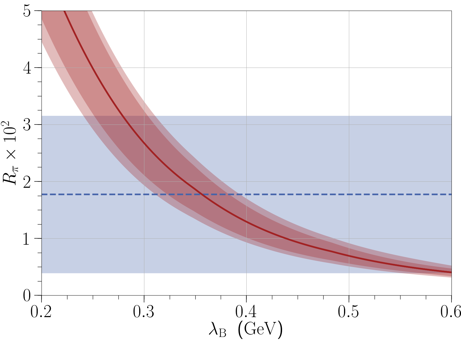
The key improvements of the presented analysis are an improved $\mathup{{{B}}}$ tagging algorithm, the Full Event Interpretation[5] (FEI), improved modeling of the background arising from semileptonic $\mathup{{{B}}}$ decays, and a new method to determine the upper limit on $\lambda_{\mathup{{{B}}}}$ via the ratio

where the dependence on $|V_{\mathrm{ub}}|$ cancels. The theory prediction and measured ratio for $R_{\mathup{{{\pi}}}}$ is shown in Figure 2. For a detailed description of the analysis see Reference [6]. The determined upper limit of the partial branching ratio with $E_{\mathup{{{\gamma}}}}>1\,\text{GeV}$ is

resulting in an upper limit of

The branching ratio of the decay $\mathup{{{B}}}\rightarrow\mathup{{{\mu}}}\mathup{{{\nu}}{}_{\scriptstyle{\!\mu}}}$ can be calculated within the SM and is predicted to be

The tree level Feynman diagram of the process is shown on the left of Figure 3.

From Equation 6 it is apparent that the decay is both helicity and CKM suppressed, which results in the small branching ratio of $\mathcal{B}(\mathup{{{B}}}\rightarrow\mathup{{{\mu}}}\mathup{{{\nu}}{}_{\scriptstyle{\!\mu}}})_{\text{SM}}\approx(4.26\pm 0.7)\cdot 10^{-7}$. Although rare, the decay has a very clean experimental signature of a high energetic monochromatic lepton momentum. Models beyond the SM can influence this branching ratio and/or the nominal momentum of the lepton. In the following two models are discussed.

Within the 2 Higgs Doublet Models (2HDM) the SM Higgs sector is extended by an additional Higgs doublet, which results in a total of five Higgs bosons after electroweak symmetry breaking, including a charged Higgs boson which can mediate the decay $\mathup{{{B}}}\rightarrow\mathup{{{\mu}}}\mathup{{{\nu}}{}_{\scriptstyle{\!\mu}}}$. The leading order Feynman diagram where the charged Higgs mediates the decay is shown in the middle of Figure 3. Depending on the parameters of the 2HDM model, the interference between the SM and 2HDM processes is either constructive or destructive, modifying the experimental signature by enhancing or reducing the observed branching ratio. In this manuscript we investigate the type-II and type-III 2HDM models[7, 8, 9], where the modification of the branching ratio is given by

with the ratio of the vacuum expectation values of the two Higgs Doublets $\tan\beta$ and the mass of the charged Higgs boson $m_{\mathup{{{H}}^{\scriptstyle{+}}}}$, and

where the coefficients $\text{C}_{\text{R/L}}$ encode the new physics contribution.

The search for the decay $\mathup{{{B}}}\rightarrow\mathup{{{\mu}}}\mathup{{{\nu}}{}_{\scriptstyle{\!\mu}}}$ allows to search for a sterile neutrino in the final state in a model independent way. One possible realization with a Leptoquark as mediator is shown on the right of Figure 3. The only requirement imposed on the sterile neutrino is a lifetime large enough to not decay inside of the detector volume. With a massive sterile neutrino in the final state, the signal peak of the monochromatic lepton momentum shifts to lower energies, thus revealing a second signal contribution in the lepton momentum spectrum, or an enhancement of the measured branching ratio if the two signal peaks are indistinguishable.

The key improvements of the presented analysis are an inclusive tagging approach with a dedicated calibration to improve the momentum resolution, which allows to measure the monochromatic signal peak in the parent $\mathup{{{B}}}$ meson, an improved description of the semileptonic $\mathup{{{B}}}\rightarrow X_{\mathup{{{u}}}}\mathit{{\ell}{}_{\mspace{-3mu}\scriptstyle{}}^{\mspace{-1mu}\scriptstyle{}}}\mathit{{\nu}{}_{\mspace{-3mu}\scriptstyle{}}^{\mspace{-1mu}\scriptstyle{}}}$ decays and an improved modeling the continuum background. For a detailed description see the upcoming publication of the analysis. The measured branching ratio is

with a significance of 2.8 standard deviations over the background only hypothesis. The allowed region for the type-II and type-III 2HDM model parameters are calculated with the measured central value of the branching ratio and are shown in Figure 4.

The scan for a sterile neutrino in the measured lepton momentum spectrum was performed by fixing the SM process to its expectation. The local $p_{0}$ value in the scanned mass range is shown in Figure 5. No significant excess was observed.

The decays $\mathup{{{B}}}\rightarrow\mathup{{{K}}^{\scriptstyle{\ast}}}\mathit{{\ell}{}_{\mspace{-3mu}\scriptstyle{}}^{\mspace{-1mu}\scriptstyle{+}}}\mathit{{\ell}{}_{\mspace{-3mu}\scriptstyle{}}^{\mspace{-1mu}\scriptstyle{-}}}$ have been studied intensively and the experimental results suggest that the underlying $\mathup{{{b}}}\rightarrow\mathup{{{s}}}\mathit{{\ell}{}_{\mspace{-3mu}\scriptstyle{}}^{\mspace{-1mu}\scriptstyle{}}}\mathit{{\ell}{}_{\mspace{-3mu}\scriptstyle{}}^{\mspace{-1mu}\scriptstyle{}}}$ transition could be affected by BSM physics in the final state containing muons[11, 12, 13, 14, 15]. The ratio of branching ratios

is well suited for testing lepton flavor universality[16]. In the SM the ratio is predicted to be close to unity, i.e. the coupling of the gauge boson does not distinguish between electrons and muons. The theoretical uncertainties originating from the form factors of the hadronic transition cancel in the ratio, making it an excellent probe for new physics.[17] In Figure 6 the leading order SM process is shown together with a possible new physics model involving a $Z^{\prime}$ boson.

The key improvements of the presented analysis are an improved reconstruction of the decay with a hierarchical neural network approach and the optimization of the analysis to measure the ratio and not the individual branching ratios. Additionally, the presented analysis includes for the first time the final state with a $\mathup{{{K}}^{\scriptstyle{\ast}}}^{+}$ meson, i.e. the measurement of the ratio $R_{\mathup{{{K}}^{\scriptstyle{\ast}}}^{+}}$. For a detailed description of the analysis see Reference [10]. The measured ratio of $R_{\mathup{{{K}}^{\scriptstyle{\ast}}}}$ over the whole $q^{2}$ range is

The value of $R_{\mathup{{{K}}^{\scriptstyle{\ast}}}}$ in individual bins of $q^{2}$ is shown in Figure 7 and tabulated in Table 1.

References

• [1] M. Beneke and J. Rohrwild, Eur. Phys. J. C 71, 1818 (2011)
• [2] A. G. Grozin and M. Neubert, Phys. Rev. D 55, 272 (1997)
• [3] M. Beneke, G. Buchalla, M. Neubert and C. T. Sachra-jda, Nucl. Phys. B 591, 313 (2000)
• [4] M. Beneke and T. Feldmann, Nucl. Phys. B 592, 3 (2001)
• [5] Keck, T., et al. Comput Softw Big Sci 3, 6 (2019)
• [6] M. Gelb et al. (Belle Collaboration) Phys. Rev. D 98, 112016 (2018)
• [7] W.-S. Hou Phys. Rev. D 48, 2342 (1993)
• [8] C.-H. Chen and T. Nomura Phys. Rev. D 98, 095007 (2018)
• [9] A. Crivellin, C. Greub, and A. Kokulu Phys. Rev. D 86, 054014 (2012)
• [10] S. Wehle et al. (Belle Collaboration) arXiv , 1904.02440v2 (2019)
• [11] S. Wehle et al. (Belle Collaboration) Phys. Rev. Lett. 118, 111801 (2017)
• [12] R. Aaij et al. (LHCb Collaboration) Phys. Rev. Lett. 113, 151601 (2014)
• [13] R. Aaij et al. (LHCb Collaboration) JHEP 02, 104 (2016)
• [14] R. Aaij et al. (LHCb Collaboration) JHEP 08, 055 (2017)
• [15] J. P. Lees et al. (BaBar Collaboration) Phys. Rev. D 86, 032012 (2012)
• [16] G. Hiller and M. Schmaltz JHEP 02, 044 (2015)
• [17] C. Bouchard et al. (HPQCD Collaboration) Phys. Rev. Lett. 111, 162002 (2013)