On the Performance of Low-Altitude UAV-Enabled Secure AF Relaying with Cooperative Jamming and SWIPT
Abstract
This paper proposes a novel cooperative secure unmanned aerial vehicle (UAV) aided transmission protocol, where a source (Alice) sends confidential information to a destination (Bob) via an energy-constrained UAV-mounted amplify-and-forward (AF) relay in the presence of a ground eavesdropper (Eve). We adopt destination-assisted cooperative jamming (CJ) as well as simultaneous wireless information and power transfer (SWIPT) at the UAV-mounted relay to enhance physical-layer security (PLS) and transmission reliability. Assuming a low altitude UAV, we derive connection probability (CP), secrecy outage probability (SOP), instantaneous secrecy rate, and average secrecy rate (ASR) of the proposed protocol over Air-Ground (AG) channels, which are modeled as Rician fading with elevation-angel dependent parameters. By simulations, we verify our theoretical results and demonstrate significant performance improvement of our protocol, when compared to conventional transmission protocol with ground relaying and UAV-based transmission protocol without destination-assisted jamming. Finally, we evaluate the impacts of different system parameters and different UAV’s locations on the proposed protocol in terms of ASR.
Index Terms:
UAV relaying, wireless information and power transfer, physical layer security, jamming.I Introduction
Unmanned aerial vehicle (UAV) based wireless communications has recently attracted significant research attentions, since it is envisioned to play a paramount role in establishing and/or improving ubiquitous and seamless connectivity of communication devices as well as enhancing capacity of future wireless networks [1, 2, 3, 4, 5].
UAVs have been introduced as aerial relays (see [6, 7, 8, 9] and references therein) in support of long-distance data transmissions from source to destination in heavily shadowed environments and/or highly overloaded scenarios. Typically, due to UAVs mobility, UAVs require a sufficiently high energy resources, which can be supported via energy harvesting techniques such as wireless energy harvesting (WEH) [10] as well as simultaneous wireless information and power transfer (SWIPT) [11]. WEH harvests energy in a controlled manner from the ambient radio-frequency (RF) signals, while SWIPT not only captures information signals, but also harvests energy of the same signals concurrently [11, 12]. Specifically, a power splitting (PS) architecture is required to divide the received signal into two separate streams of different power levels, one for signal processing and the other for simultaneous energy harvesting [13].
One technical challenge of UAV-assisted communications is to guarantee physical layer security. The unique characteristics of Air-Ground (AG) channels can provide good channel condition for legitimate nodes, but, on the other hand, is prone to eavesdropping by non-legitimate nodes [14, 15]. Exploiting PLS techniques in UAV-assisted communications has been studied in [16, 17, 18, 19] (see references therein). In [16], the authors have studied PLS of a UAV-enabled mobile relaying scheme over non-fading AG channels, and showed that moving buffer-aided relay provides significant performance over static relaying in terms of secrecy rate. In [17], the authors studied the resource allocation and path-planning problem for energy-efficient secure transmission from a UAV base station to multiple users in the presence of a passive ground eavesdropper. In [18], employing UAV as a friendly jammer to enhance PLS of a ground-relaying based communication has been studied. In [19], the authors have examined SWIPT-enabled secure transmission of millimeter wave (mmWave) for a UAV relay network, where the UAV feeds the energy-constrained IoT destination device in the presence of multiple ground eavesdroppers while a free-space path loss (PL) model for AG links was adopted.
In this paper, we consider a practical scenario where a low-altitude UAV relaying is employed to assist communications between source and destination nodes. Based on the recent channel measurements in [20, 21], low-altitude UAV relay channels may also suffer from small scale fading compared to high-altitude cases. Hence, we assume that AG channel models are Rician fading of different parameters. Then, we tackle the aforementioned security and energy limitation challenges and we make the following contributions.
- •
We propose a secure and energy-efficient transmission protocol, where a source sends confidential information to a destination via an energy-constrained UAV-mounted amplify-and-forward (AF) relay in the presence of a passive eavesdropper. In the protocol, we adopt the destination-assisted cooperative jamming (CJ) and SWIPT techniques at the UAV based relay for PLS improvements as well as energy harvesting.
- •
We analyze the proposed secure transmission protocol in terms of reliability and security. In particular, we derive connection probability, secrecy outage probability, instantaneous secrecy rate, and average secrecy rate of the proposed protocol from source to destination via relay.
- •
We conduct simulations to verify our theoretical results, identify the best location of the UAV based relay that provides the best average secrecy rate, evaluate impacts of different system parameters on the system performance in terms of reliability and security, and finally validate the effectiveness and improvements of the proposed protocol, when compared to convectional transmission protocol with ground relaying and UAV-based transmission protocol without destination-assisted jamming.
The rest of this paper is organized as below. Section II presents system model and channel model. In Section III, we propose the UAV-based transmission protocol with destination-assisted jamming and SWIPT techniques. In Section IV, we conduct performance analysis. Numerical results are given in Section V, and finally, conclusions are drawn in Section VI.
II System Model and Channel Model
In this section, we introduce system model and channel model.
II-A System Model
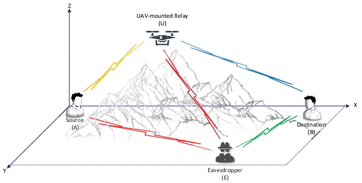
We consider a point-to-point secure transmission scheme (see Fig. 1), where we employ a UAV-mounted relay () to assist confidential transmission from a source node to a legitimate destination node over heavily shadowed areas in the presence of a ground passive eavesdropper . The locations of source, destination, and eavesdropper are fixed on the ground with their 3D coordination: , , , while UAV is located at and is its altitude from ground surface.
We assume that all nodes with a single antenna operate in a half-duplex mode and the UAV relay node () adopts AF protocol. Further, we assume the relaying node () uses simultaneous wireless information and power transfer (SWIPT) technology to harvest energy from the received radio frequency (RF) signals transmitted by and , while it also uses its on-board battery for maneuvering and staying stationary in the sky. Finally, we assume that the UAV receiver adopts power splitting architecture (see Fig. 2), where () is the power splitting ratio (PSR) identifying the portion of the harvested power from the received RF signals and denotes the PSR for signal processing at the AF relay.

II-B Channel Model
Here we consider both small-scale fading and large-scale PL in setting up the channel model. We assume the channel between and the ground node {, , } is Rician fading but with different values of Rice parameters. Exploiting channel reciprocity, the normalized channel power gain between the links , , and denoted by
| (1) |
follow a square Rice distribution (i.e., non-central chi-square (nc-) distribution) with two degrees of freedom, corresponding to line-of-sight (LOS) and non-line-of-sight (NLOS) components whose probability density function (PDF) and cumulative distribution function (CDF) are
| (2) |
and
| (3) |
where holds any non-negative value, and denote the PDF and the CDF for the link, and represents the modified Bessel function of the first kind and zero-order, (in dB) is the K-factor given by [22]
| (4) |
where and are two constants depending on the environment and transmission frequency, (in radian) is the elevation angle between two given nodes.
Furthermore, we assume the channel model between ground nodes is Rayleigh fading, a special case of Rician fading with , and thus the channel power gain for the links , , and , can be modeled as exponential distribution with unit scale parameters.
For large scale PL, considering the probability of LOS [23], we adopt elevation-angle dependent PL component
| (5) |
where and represent PL exponents for LOS links between two nodes (), and NLOS links (), respectively, and and are environmental constants. Letting be the Euclidean distance between two nodes, we let as the PL model. Note that for G2G links with , the PL model follows only NLOS components, however, for AG links the PL component is between and depending on the elevation-angel between nodes.
III Proposed Transmission Protocol

We consider the following two equal-duration phase secure transmission protocol with an overall duration seconds (Fig. 3). During the first time slot, sends information signal to and simultaneously, transmits a jamming signal to degrade the wiretap channel of as well as to assist the energy harvesting of UAV. Then the AF relay receives
| (6) |
where and denote the normalized information signal from , and jamming signal from , i.e.,
and and represent transmit power from and jamming power from , which satisfy
| (7) |
and is fixed for each frame. Further, we assume
| (8) |
where is the power allocation factor. Besides, represents signal processing noise at the power splitting component with power , and is the Additive white Gaussian noise (AWGN) at . The energy harvested by from the received signals can be written as
| (9) |
where is the power conversion efficiency factor for the harvester. Here, we assume that the total harvested energy during the first phase will be used for signal transmission in the second phase and is given by
| (10) |
Different from [16] where no direct link was assumed to exists from to , here we consider a more general scenario during which may also overhear the confidential messages from to due to broadcast nature of wireless media. Specifically, if is located on the ground that is in not so far from , can attempt to decode the received signal information based on the received signal-to-interference-plus-noise ratio (SINR)
| (11) |
In the second phase, forwards the scaled version of to with the amplification factor
| (12) |
where is in (10). The resultant signal at the node {, } can be expressed as
| (13) |
Owning to the fact that is assumed to be able to conduct full self-interference cancellation, hence the term of jamming interference can be canceled from (III), whereas acts with this part as an interference. Therefore, the received SINR at and can be obtained as
| (14) |
and
where
| (18) |
IV Performance Analysis
In this section, we derive connection probability, secrecy outage probability, instantaneous secrecy rate, as well as achievable average secrecy rate of the proposed transmission protocol. In the derivations, we assume that the channel coefficients between nodes remain constants during each frame and vary from one frame to next independently.
IV-A Connection Probability
Definition 1.
The connection probability (CP), i.e., the probability that is able to decode the transmitted signal from and correctly extract the secure information messages [24], is defined as
| (20) |
where
| (21) |
and denote the instantaneous capacity and transmission rate of - via , which is normalized by bandwidth as [25], where is given by (14).
The following theorem provides an analytical closed-form expression of .
Theorem 1.
We derive the CP of the secure UAV-based relaying in (1), where , and are two positive integers controlling the accuracy of (1), represents the gamma function, is given in (18), are dummy variables, , is given in (4), and is the modified Bessel function of the first kind with the order of .
| (22) |
Proof.
See Appendix A. ∎
IV-B Secrecy Outage Probability
Following [26], when the instantaneous capacity of the wiretap link , defined as
| (23) |
is larger than the rate difference , where is rate of the confidential information from - via , then the secrecy outage occurs and the eavesdropper is able to intercept the transmitted confidential information via . The analytical expression for is given by Theorem below.
IV-C Instantaneous Secrecy Rate
Definition 2.
Note that we assume that the channel coefficients between nodes remain constants during each frame and vary from one frame to next independently. Then all parameters in (2) are assumed to be known except the power allocation factor , thereby we form the following optimization problem
Considering is guaranteed under optimal power allocation, the above optimization problem is equivalent to finding the optimal power allocation factor, i.e.,
| (29) |
where
| (30) |
which is due to the fact that in (2) is a strictly increasing function w.r.t , and thus (29) can be solved analytically in the high SNR regime as given in Theorem 3.
Theorem 3.
In large SNR regime, the function in (30) is proven to be quasi-concave w.r.t in the feasible set where and can be obtained as
| (31) |
where .
Proof.
See Appendix C. ∎
IV-D Achievable Average Secrecy Rate
Definition 3.
The achievable average secrecy rate (ASR) is defined as
| (32) |
Averaging over all realizations of the channels yields in (IV-D).
| (33) |
Owning to the fact that the exact computation of (IV-D) is an arduous task and hence, instead, we derive a tight lower-bound for ASR in the Theorem below. First, we present the following worthwhile lemma, by which we then delve into the derivation of the closed-form lower-bound for the ASR in Theorem 4.
Lemma 1.
Let be a non-central chi-square random variable with two degrees of freedom and the non-centrality parameter , also holds non-negative values, then the expectation of the new random variable , can be obtained as follows.
| (34) |
where and are defined respectively as
| (35) |
where is some positive integer and the coefficients and are given, as finite series, respectively, by
| (36) |
and
| (37) |
wherein and are the Gamma function and the Psi function respectively defined as and [27]. Moreover, the function in (37) is given by (see (1))
| (38) |
Theorem 4.
The lower bound of the average secrecy rate of the proposed secure UAV-enabled relaying system is given by
| (39) |
with
| (40) |
| (41) |
Proof.
See Appendix D. ∎
V Numerical Results and Discussions
In this section, we present simulation results of connection probability, secrecy outage, and average secrecy rate in order to validate our theoretical results in the paper. We also demonstrate both reliability and security performance enhancements offered by UAV-based relaying (UR) and destination-assisted CJ transmission protocol, compared to the case using ground relaying (GR), and the case using UR but without destination-jamming.
Unless otherwise stated, we consider the following system parameters in all simulations. We assume =10 (the normalized distance of - w.r.t m), =1.5 (the normalized height at which UAV operates w.r.t m). We assume the nodes locations: , , , . The path-loss exponents are =2 and =3.5, respectively. Besides, the network transmission rate =0.5 bits/s/Hz, the secrecy rate =0.2 bits/s/Hz are adopted. Further, we assume , , energy harvesting efficiency factor , , , , and [23, 21, 28]. Also, the EPSA represents equal power allocation (i.e., ) and equal power splitting ratio (i.e., ). The Monte-Carlo simulation are obtained through averaging over realizations of the channel coefficients.
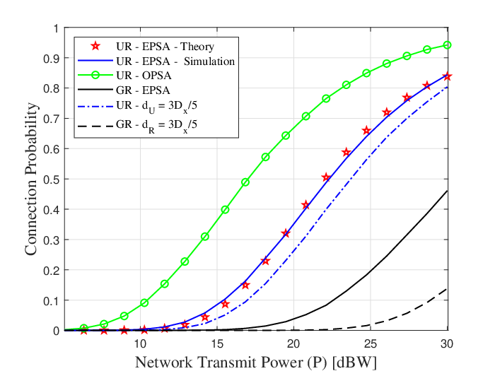
Fig. 4 illustrates the CP in (1) for the proposed transmission protocol with EPSA and OPSA, respectively, against the network transmit power . Here, OPSA refers to the case with optimal and for a given , represents the horizontal projection distance of to , and is the distance from the ground relay to source. Here for a fair comparison, we assume . We can observe that the CP of OPSA-based scheme gets approximately doubled, compared to EPSA-based one, in the practical range of transmit power, e.g., for dBW. The figure compares the simulated CP and theoretical CP in (1) of the proposed protocol with EPSA and demonstrates that they are well matched. Fig. 4 also illustrates a significant CP improvement of the proposed protocol, when compared to the case using ground relaying, under the setting of EPSA.

Fig. 5 illustrates the simulated and theoretical SOP versus network transmit power for the proposed protocol using CJ with and demonstrates they are well matched. The figure also compares the proposed protocol, the UAV based relaying without any security technique and the one using ground relaying, and demonstrates the effectiveness of our protocol in terms of SOP thanks to the joint effect of destination CJ and SWIPT.

Fig. 6 compares the lower bound of ASR (see Theorem 4) with different truncated values (see Theorem 4) and the simulated result using the exact expression (IV-D). We can see that they are very close, especially when dBW. Further, we observe that normalizing the gap between the exact value and the lower bound w.r.t the exact value yields the relative errors of , , and for the cases of , , and, , respectively. This demonstrates the finite series we obtained are acceptably valid while explicitly truncated.

Fig. 7 depicts the impact of and on ASR. Given a fixed power budget dBW, the ASR increases when and increase. The best ASR can be obtained at and . A higher (i.e., higher ) provides higher reliability of data transmission, but when , ASR decreases slightly. This is due to the fact that a high source power can enhance and a low jamming power is sufficient to degrade eavesdropper. Overall, the plot provides a good trade-off between source power and destination jamming power in terms of ASR.

Fig. 8 shows ASR against normalized horizontal distance of the proposed protocol with and without destination CJ for different values. Here normalized horizontal distance is defined as the ratio of the horizontal distance of (-) to that of (-). This scenario can be viewed as a relay moving from the initial location above with a direct path to the final location right above and we are seeking the best location of in terms of ASR.
From Fig. 8, we observe that the proposed protocol with CJ outperforms the one without CJ, and particularly, the proposed protocol with CJ and leads to the best ASR, compared to other values, over all different normalized horizontal distances. Also, we observe the best location of is . This is due to the fact that when is near and far from , we need to allocate more to enhance for source transmission and less , which is sufficient for destination CJ. When is at the location of (i.e., is in the vicinity of eavesdropper), the wiretap link obviously reduces the ASR. Last but not least, when is within (), more proportion of the power budget should be dedicated for jamming in order to improve ASR.

Fig. 9 displays ASR against UAV altitude for the proposed protocol with different . Firstly, we observe that and yield the best ASR among all. Secondly, we observe, when increases till , ASR increases to the peak, and after that, ASR decreases. This is due to the fact that, from onwards, the attenuation factor caused by the ’s long distance from the ground nodes significantly affects the ASR. When , the ASR is a quasi-concave function having one optimal value for given system parameters. Furthermore, for is in low altitude, e.g., , increasing (i.e., a larger proportion of the received power is stored for EH which is then utilized in AF relaying), yields improved ASR. For higher altitudes, the ASR increases if , or decreases if , where . This is due to the fact that, when , large UAV transmission power can lead to the improved received SNR at , but this also yields better signal reception at Eve.
VI Conclusions
In this paper, we proposed a secure and energy-efficient source-UAV-destination transmission protocol with the aid of destination cooperative jamming and SWIPT at the relay, when a passive eavesdropper exists. We derived the connection probability, secrecy outage probability, instantaneous secrecy rate, and average secrecy rate of the proposed transmission protocol from to via a stationary and verified them via simulations. Further, by simulations, we demonstrate significant performance improvement of our protocol, when compared to conventional transmission protocol with ground relaying and UAV-based transmission protocol without destination-assisted jamming. We also identified the best location of that provides the optimal ASR, given a fixed eavesdropper location. Finally, we evaluated the impacts of different system parameters on the system performance. For future work, we will consider the extension to flying UAV relaying with extra degrees of freedom in the system design.
Appendix A Derivation of Connection Probability
| (A.1) |
where , ,
and is the first-order Marqum Q-function, and is the modified Bessel function of the first kind with th order. Furthermore, follows from plugging the approximate expressions for and given respectively as [29]
| (A.2) |
and
| (A.3) |
Finally, applying the equation [27, Eq. (3.471.9)] for calculating the integral expression of the last equation of (A), one can reach, after tedious manipulations, at (1) and so the proof is done.
Appendix B Derivation of Secrecy Outage Probability
To obtain we need to calculate and . Henceforth, in order to calculate , let define and while rewriting (25) as
| (B.1) |
calculating the last integral results in (25).
Now, we focus on obtaining an analytical expression for as follows. By defining the auxiliary variables , , , and letting , , and , one can rewrite given in (2) as
| (B.2) |
where in which , , . Then, is calculated in a closed-form expression using (A.3) given in Appendix A as (see (B)).
| (B.3) |
| (B.4) |
in which , . Moreover, comes from using [27, Eq. (6.643.2)] to calculate the integral term, wherein is the Whittaker M-function. Next, in order to obtain a closed-form expression for the single-form integral given by (B) we further calculate as (see (B)), where , , , , and denotes the modified Bessel function with the second kind and -th order. Note that the above equation achieved by applying [27, Eq. (3.478.4)]. Finally, through tedious mathematical manipulations we can achieve the closed-form expression for the SOP given by (2), and hence, the proof is done.
Appendix C Derivation of optimal
Taking the auxiliary variables
we rewrite the function , considering high Transmit SNR approximation, as
| (C.1) |
where , , . Now, taking the first derivation of the function w.r.t , i.e., results a rational polynomial function with always-positive denominator and the numerator of forth-order, where it can readily be found that and are the roots of both and its first derivative . Hence the remained two roots are the solutions of the second order polynomial given as
| (C.2) |
where . As such, considering the feasible set of , we have three cases as
- 1.
, no optimum solution
- 2.
,
- 3.
,
Furthermore, note that it is easy to prove holds positive values in and are negative in and the extremum determines the maximum of the [30], and hence the proof is complete.
Appendix D Derivation of Lower-bounded ASR
In order to obtain a closed-form lower-bound expression for , one can write, following the Jensen’s inequality, as [31] (see (D)).
| (D.1) |
In (D), the term is further calculated as
| (D.2) |
where can be analytically obtained using Lemma 1 as given in (4). Letting , the remained parts and in (D) are derived as
| (D.3) |
| (D.4) |
where is the exponential integral, follows from the approximate given in [32] along considering the tight lower bound for given in [33]. However that can be readily obtained inasmuch as it equals to the first derivative of , already given in (1), w.r.t , we use this tight approximation for simplicity.
References
- [1] Y. Zeng, R. Zhang, and T. J. Lim, “Wireless communications with unmanned aerial vehicles: Opportunities and challenges,” IEEE Commun. Mag., vol. 54, no. 5, pp. 36–42, 2016.
- [2] S. Hayat, E. Yanmaz, and R. Muzaffar, “Survey on unmanned aerial vehicle networks for civil applications: A communications viewpoint,” IEEE Commun. Surveys Tuts., vol. 18, no. 4, pp. 2624–2661, 2016.
- [3] F. Cheng, G. Gui, N. Zhao, Y. Chen, J. Tang, and H. Sari, “UAV relaying assisted secure transmission with caching,” IEEE Trans. Commun., pp. 1–1, 2019.
- [4] B. Li, Z. Fei, and Y. Zhang, “UAV communications for 5G and beyond: Recent advances and future trends,” IEEE Internet Things J., pp. 1–1, 2018.
- [5] X. Liu, Z. Li, N. Zhao, W. Meng, G. Gui, Y. Chen, and F. Adachi, “Transceiver design and multi-hop D2D for UAV IoT coverage in disasters,” IEEE Internet Things J., pp. 1–1, 2019.
- [6] D. H. Choi, S. H. Kim, and D. K. Sung, “Energy-efficient maneuvering and communication of a single UAV-based relay,” IEEE Trans. Aerosp. Electron. Syst., vol. 50, no. 3, pp. 2320–2327, July 2014.
- [7] Y. Zeng, R. Zhang, and T. J. Lim, “Throughput maximization for UAV-enabled mobile relaying systems,” IEEE Trans. Commun., vol. 64, no. 12, pp. 4983–4996, 2016.
- [8] S. Zeng, H. Zhang, K. Bian, and L. Song, “UAV relaying: Power allocation and trajectory optimization using decode-and-forward protocol,” in Proc. IEEE ICC, May 2018, pp. 1–6.
- [9] M. Hua, Y. Wang, Z. Zhang, C. Li, Y. Huang, and L. Yang, “Outage probability minimization for low-altitude UAV-enabled full-duplex mobile relaying systems,” China Commun., vol. 15, no. 5, pp. 9–24, May 2018.
- [10] X. Lu, P. Wang, D. Niyato, D. I. Kim, and Z. Han, “Wireless networks with rf energy harvesting: A contemporary survey,” IEEE Commun. Surveys Tuts., vol. 17, no. 2, pp. 757–789, 2015.
- [11] T. D. Ponnimbaduge Perera, D. N. K. Jayakody, S. K. Sharma, S. Chatzinotas, and J. Li, “Simultaneous wireless information and power transfer (SWIPT): Recent advances and future challenges,” IEEE Commun. Surveys Tuts., vol. 20, no. 1, pp. 264–302, 2018.
- [12] L. Yang, J. Chen, M. O. Hasna, and H.-C. Yang, “Outage performance of UAV-assisted relaying systems with rf energy harvesting,” IEEE Commun. Lett., vol. 22, no. 12, pp. 2471–2474, 2018.
- [13] Q. Wu, G. Y. Li, W. Chen, D. W. K. Ng, and R. Schober, “An overview of sustainable green 5G networks,” IEEE Wireless Commun., vol. 24, no. 4, pp. 72–80, 2017.
- [14] Y. Zou, J. Zhu, X. Wang, and L. Hanzo, “A survey on wireless security: Technical challenges, recent advances, and future trends,” Proc. IEEE, vol. 104, no. 9, pp. 1727–1765, 2016.
- [15] Q. Wu, W. Mei, and R. Zhang, “Safeguarding wireless network with UAVs: A physical layer security perspective,” arXiv preprint arXiv:1902.02472, 2019.
- [16] Q. Wang, Z. Chen, W. Mei, and J. Fang, “Improving physical layer security using UAV-enabled mobile relaying,” IEEE Wireless Commun. Lett., vol. 6, no. 3, pp. 310–313, 2017.
- [17] Y. Cai, Z. Wei, R. Li, D. W. K. Ng, and J. Yuan, “Energy-efficient resource allocation for secure UAV communication systems,” arXiv preprint arXiv:1901.09308, 2019.
- [18] Y. Wang, W. Yang, X. ShaYuan, and Y. Cai, “Energy-efficient secure transmission for UAV-enabled wireless powered communication,” in Proc. 10th Int. Conf. Wireless Commun. Signal Process. (WCSP), Oct 2018, pp. 1–5.
- [19] X. Sun, W. Yang, Y. Cai, Z. Xiang, and X. Tang, “Secure transmissions in millimeter wave SWIPT uav-based relay networks,” IEEE Wireless Commun. Lett., pp. 1–1, 2019.
- [20] R. Amorim, H. Nguyen, P. Mogensen, I. Z. Kovacs, J. Wigard, and T. B. Sorensen, “Radio channel modeling for UAV communication over cellular networks,” IEEE Wireless Commun. Lett., vol. 6, no. 4, pp. 514–517, 2017.
- [21] A. A. Khuwaja, Y. Chen, N. Zhao, M.-S. Alouini, and P. Dobbins, “A survey of channel modeling for UAV communications,” IEEE Commun. Surveys Tuts., vol. 20, no. 4, pp. 2804–2821, 2018.
- [22] M. M. Azari, F. Rosas, K. Chen, and S. Pollin, “Ultra reliable UAV communication using altitude and cooperation diversity,” IEEE Trans. Commun., vol. 66, no. 1, pp. 330–344, 2018.
- [23] Y. Zhu, G. Zheng, and M. Fitch, “Secrecy rate analysis of UAV-enabled mmWave networks using Matérn Hardcore point processes,” IEEE J. Sel. Areas Commun., vol. 36, no. 7, pp. 1397–1409, 2018.
- [24] M. T. Mamaghani and R. Abbas, “Security and reliability performance analysis for two-way wireless energy harvesting based untrusted relaying with cooperative jamming,” IET Commun., vol. 13, no. 4, pp. 449–459, 2019.
- [25] J. N. Laneman, D. N. C. Tse, and G. W. Wornell, “Cooperative diversity in wireless networks: Efficient protocols and outage behavior,” IEEE Trans. Inf. Theory, vol. 50, no. 12, pp. 3062–3080, 2004.
- [26] J. Yao and J. Xu, “Secrecy transmission in large-scale UAV-enabled wireless networks,” arXiv preprint arXiv:1902.00836, 2019.
- [27] I. S. Gradshteyn and I. M. Ryzhik, Table of integrals, series, and products. Academic press, 2014.
- [28] M. T. Mamaghani, A. Mohammadi, P. L. Yeoh, and A. Kuhestani, “Secure two-way communication via a wireless powered untrusted relay and friendly jammer,” in Proc. IEEE Global Commun. Conf., Dec 2017, pp. 1–6.
- [29] K. Cao and X. Gao, “Solutions to generalized integrals involving the generalized marcum -function with application to energy detection,” IEEE Commun. Lett., vol. 20, no. 9, pp. 1780–1783, Sep. 2016.
- [30] S. Boyd and L. Vandenberghe, Convex optimization. Cambridge university press, 2004.
- [31] M. Tatar Mamaghani, A. Kuhestani, and K.-K. Wong, “Secure two-way transmission via wireless-powered untrusted relay and external jammer,” IEEE Trans. Veh. Technol., vol. 67, no. 9, pp. 8451–8465, 2018.
- [32] E. Bjornson, M. Matthaiou, and M. Debbah, “A new look at dual-hop relaying: performance limits with hardware impairments,” IEEE Trans. Commun., vol. 61, no. 11, pp. 4512–4525, November 2013.
- [33] S. M. Moser, “Expectations of a noncentral Chi-square distribution with application to i.i.d MIMO Gaussian fading,” in Proc. IEEE ISIT, Dec 2008, pp. 1–6.