Sticky Brownian Motion
and its Numerical SolutionThanks: 

Consider a diffusion process $X^{\epsilon}_{t}$ on $\mathbb{R}_{\geq 0}$, depending on a parameter $\epsilon>0$, which solves

with a reflecting boundary condition at the origin. Here $W_{t}$ is a standard Brownian motion, and $U^{\epsilon}(x):\mathbb{R}\to\mathbb{R}$ is a function parameterized by $\epsilon$. If $X^{\epsilon}_{t}$ is the position at time $t$ of a particle moving on the real axis, then the force it feels is $-\partial_{x}U^{\epsilon}(X^{\epsilon}_{t})$. Recall that, if $\int_{0}^{\infty}e^{-U^{\epsilon}(x)}dx<\infty$, then $e^{-U^{\epsilon}(x)}$ is the non-normalized stationary (or equilibrium) probability density of $X^{\epsilon}_{t}$.

Equation (1) is a special case of the Brownian dynamics equations, which are a good model for the dynamics of mesoscale particles in a fluid [30]. For a more general system of particles, $X_{t}^{\epsilon}$ would be the configuration, a vector of particle positions, $U^{\epsilon}(x)$ would represent the potential energy of a particular configuration (nondimensionalized by temperature), which is usually a sum of the potential energy between each pair of particles, and the equations may additionally include a friction tensor, depending on the configuration and the velocity, modeling hydrodynamic interactions between particles. We specialize to a single scalar equation and ignore friction, but still think of $U^{\epsilon}(x)$ as a potential energy, representing the energy of the particle $X_{t}^{\epsilon}$ as a function of its distance to another particle. Physically, this equation could be realized by holding one particle in place at the origin while another is particle moves on a line.

An important point is that for mesoscale particles, $U^{\epsilon}(x)\approx 0$ outside an interval that is very narrow compared to the particles’ diameters [70, 41]. For example, for particles interacting with a so-called “depletion” interaction [4], the range of the interaction in a typical experiment was estimated to be about 5% of the particles’ diameters [71]. Therefore, when two particles’ surfaces are within this range of each other, they stay close together for a long time, but when they are further apart they don’t feel each other at all, and diffuse independently. An even shorter range is achieved by particles that interact via sticky single-stranded DNA coated on their surfaces: here, the range of the interaction is the average radius of a coiled DNA strand, which is typically around 10nm, about 1% of the diameter of a 1$\mu$m particle [90]. Such DNA-coated particles are studied extensively because the DNA allows one to code complex interactions between different types of particles, and hence, to program them to assemble into a great many different materials [68, 12, 90, 83, 95].

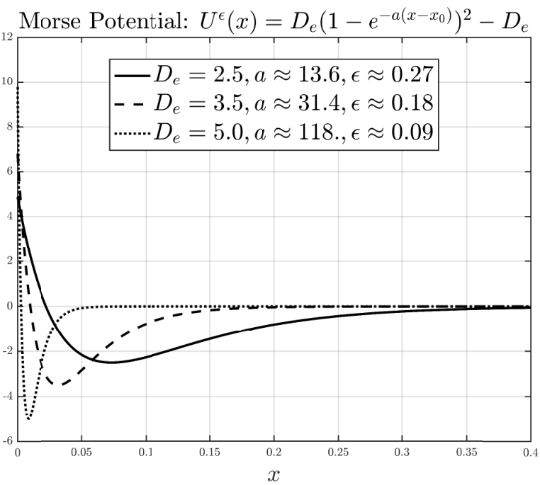
With these remarks in mind, we consider a family of potential energy functions $(U^{\epsilon}(x))_{\epsilon>0}$ with a narrow, deep attractive well, which becomes narrower and deeper as $\epsilon\to 0$. We consider the dynamics of $X^{\epsilon}_{t}$ as $\epsilon\to 0$, and call this the sticky limit. Specifically, we impose the following assumptions on $(U^{\epsilon}(x))_{\epsilon>0}$.

We briefly comment on the physical interpretation of (A1)-(A3). Assumption (A1) ensures the potential and its first two derivatives are negligible outside of the interval $(0,\epsilon)$, which we call the boundary layer. Outside the boundary layer, $X^{\epsilon}_{t}$ feels virtually no force and simply diffuses.

Assumption (A2) ensures that the dynamics in (1) has at most one timescale within the boundary layer. A typical timescale for a diffusion process is its mean first passage time (MFPT) to overcome an energy barrier $\Delta U$. Under Assumption (A2), the barrier to leaving the interval $(0,\epsilon)$ is the depth of the potential at its minimum, leading to an MFPT of approximately $\epsilon e^{\Delta U}$ [32]. The assumption rules out pathological potentials with many large oscillations in the boundary layer, which would give rise to longer dynamical timescales in the boundary layer.

Assumption (A3) is the one that gives rise to stickiness at the origin. It requires that the measure of $(0,\epsilon)$ with respect to the weighted Lebesgue measure $e^{-U(x)}dx$, or in the language of physics, the partition function for this interval, approaches a constant. This constant $\kappa$ determines how sticky the origin is – larger $\kappa$ means the process will spend longer near the origin on average. For this reason we call $\kappa$ the sticky parameter. Applying Laplace asymptotics to (2) shows that

where $x_{0}$ is the minimizer of $U^{\epsilon}(x)$ in $(0,\epsilon)$. Ignoring the second derivative shows that the depth must scale very nearly as $|U^{\epsilon}(x_{0})|\sim|\log\epsilon|$, the logarithm of the width of the potential. This implies the timescale computed from the MFPT for leaving the boundary layer is $\epsilon e^{\Delta U}\sim O(1)$. If the scaling of the depth of the well is larger than $|\log\epsilon|$, then large deviation theory would be more appropriate to describe the dynamics of the limiting process [14, 36]. However, if the scaling is smaller, then the limiting process spends no time on the boundary, and simply reflects off of it, as we will see momentarily.

The requirement that $U^{\epsilon}$ has two derivatives is not necessary, but is included to simplify our calculations and avoid dealing with discontinuities in the coefficients of (1). An example of a potential energy function which doesn’t satisfy this condition, but which is commonly used to model short-ranged potentials, is the square-well potential.²² 2 Square-well potentials have the form $U^{\epsilon}(x)=C_{\epsilon}$ for $x\in[0,\epsilon]$, $U^{\epsilon}(x)=0$ for $x>\epsilon$, $U^{\epsilon}(x)=\infty$ for $x<0$; where $C_{\epsilon}$ is a constant which depends on $\epsilon$. By introducing a smooth approximation, we expect our asymptotic results to hold for a square-well potential as well, though we do not pursue this here.

Assumption 1 can be verified for two families of potentials frequently used to model attractive interactions between mesoscale particles, the Morse and generalized Lennard-Jones potential energy functions [18, 69, 72, 88, 11, 94].

Consider the dynamics of $X^{\epsilon}_{t}$ in (1) when $\epsilon$ is small. When $X^{\epsilon}_{t}$ is far enough away from the origin, it feels no force, and simply diffuses, like a Brownian motion. When $X^{\epsilon}_{t}$ is within a distance of $\epsilon$ from the origin, it feels a strong force keeping it near the minimum of $U^{\epsilon}$ for a long time, until an occasional large fluctuation pushes it out of the range of the force.

How long does it stay near the origin, and does this time remain significant as $\epsilon\to 0$? We start by computing the mean first-passage time (MPFT) to escape from a region near the origin.

When $\kappa=0$, we recover the MFPT of a reflecting Brownian motion starting at $0$. The time scales as the distance squared, $\tau^{\epsilon}(0)\sim O(\ell^{2})$, a traditional diffusive scaling. When $\kappa\to\infty$, the MFPT is infinite, consistent with the MFPT of an absorbing Brownian motion starting at $0$. For intermediate $\kappa$, the MFPT at the origin scales as $\tau^{\epsilon}(0)\sim O(\ell)$, which is a ballistic scaling – slower (for small $\ell$) than the diffusive scaling. Therefore, we expect the limiting probability density near the origin to be correspondingly large.

To gain further insight into the dynamics, consider the evolution of the probability density $p^{\epsilon}(x,t)$ of $X^{\epsilon}_{t}$. It evolves according to the Fokker-Planck equation

where $j^{\epsilon}(x,t)=-\partial_{x}U^{\epsilon}(x)p^{\epsilon}(x,t)-\partial_{x}p^{\epsilon}(x,t)$ is the associated probability current, or probability flux. The equation is to be solved in the domain $x>0$, $t>0$ with boundary condition $j^{\epsilon}(0,t)=0$ for all $t\geq 0$, and given initial condition $p^{\epsilon}(x,0)=\phi(x)$.

For this one-dimensional problem we could compute $p^{\epsilon}(x,t)$ to high accuracy by solving the PDE (4) numerically. However, such an approach won’t work in the high dimensions characteristic of systems of particles, so to illustrate the difficulties that may arise, we simulate $10^{6}$ trajectories of (1) numerically and estimate the density by kernel density estimation. We use a Morse potential for $U^{\epsilon}$ as in Example 2, and a symmetrized Euler-Maruyama approximation to solve (1), a method that is first-order weakly accurate method for domains with a smooth enough boundary [35, 7]. The method works as follows: given a time-step size $\delta t$, we set $t_{k}=k\delta t$ for $k\in\mathbb{N}_{\geq 0}$, and compute the approximation $\tilde{X}_{k}$ to $X^{\epsilon}(t_{k})$ as

See Appendix A for Matlab code implementing this method. Unfortunately, when the Morse potential used is short-ranged and strong, an accurate approximation requires a small time step size: when $\kappa=1,a\approx 118$ the time step size required for a qualitatively correct solution is approximately $\delta t\leq 2.5\times 10^{-6}$ – Figure 2 shows that larger timesteps fail to see the boundary layer entirely.

Figure 3 plots $p^{\epsilon}(x,1)$ on a log scale for various values of $\epsilon$, and shows that as $\epsilon$ decreases, $p^{\epsilon}(x,1)$ has an increasingly large peak in density near the origin. Although the width of the peak decreases, the total probability in the peak remains nearly constant with $\epsilon$. Therefore, we expect the probability density to contain a singularity of the form $\delta(x)$ when $\epsilon\to 0$.

Furthermore, notice that $p^{\epsilon}(x,1)$ is slowly varying for $x\geq\epsilon$ and rapidly varying for $0\leq x\leq\epsilon$. This suggests using the method of matched asymptotic expansions to study (4) as $\epsilon\to 0$ [40, 49]. This approach, which is very similar to boundary-layer theory in fluids, proceeds by finding a local ‘inner’ solution near the origin and a local ‘outer’ solution far enough away from the origin, and then matching these local solutions in an intermediate region.

We pursue the method of matched asymptotic expansions to show that the leading-order probability density of $X^{\epsilon}_{t}$ (leading-order in the sense of a measure) is

where $p(x,t)$ solves

with a given initial condition $p(x,0)=\phi(x)$. We assume that $\phi$ is continuously differentiable on $[0,\infty)$ and that $\phi$ and $\phi^{\prime}$ are bounded on $[0,\infty)$; assumptions which guarantee that (6) is well-posed [79, Theorem 1]. Equations (6), (7) are the main results of this section, and describe the evolution of probability of a SBM [27].

To derive these equations we adopt a formal approach to highlight the main ideas, but expect that the argument could be turned into a more rigorous proof of weak convergence by the interested reader.

Let us make the ansatz that the solution to (4) away from the origin ($x\geq\epsilon$), or outer solution, and near the origin ($x\leq\epsilon$), or inner solution, have the asymptotic expansions, respectively,

where $p_{0}(x,t)$ and $q_{0}(x,t)$ are the leading order terms in the expansions, and $p_{1}\ll p_{0}$, $q_{1}\ll q_{0}$ as $\epsilon\to 0$. We do not assume any particular scaling for these terms, nor the leading-order solutions; it will turn out that $p_{0}\sim O(1)$ but $q_{0}\sim O(\epsilon^{-1})$, because of Assumption 1 (A3).

By Assumption 1 (A1), the outer solution $p_{0}(x,t)$ satisfies the following linear PDE to leading order as $\epsilon\to 0$:

with $p_{0}(x,0)=\phi(x)$. Near the origin, the density changes rapidly so it is convenient to change variables to $X=x/\epsilon$. Keeping the leading-order terms gives

with the reflecting boundary condition $\partial_{X}U^{\epsilon}(0,t)q_{0}(0,t)+\partial_{X}q_{0}(0,t)=0$. We have used Assumption 1 (A2) and the timescale it implies to argue that $\partial_{t}q_{0}$ is lower order than the terms retained in (10).

Equation (10) is the equation for the stationary density of a particle diffusing in a potential $U^{\epsilon}$ with a reflecting boundary condition at the origin. The solution is

where $a(t)$ is some unknown function of time, to be determined by matching to the outer solution.

Now we match the outer solution $p_{0}(x,t)$ and the inner solution $q_{0}(\epsilon X,t)$ at $x=\epsilon$, $X=1$. Unlike the traditional method of matched asymptotic expansions, we do not match in an overlap region, but rather at a single point, which is possible because the perturbation is not singular (the diffusion terms do not change with $\epsilon$.) We match using two conditions: one, probability is continuous, and two, probability is conserved. The first condition requires that

to leading order in $\epsilon$, where we used that $e^{-U^{\epsilon}(\epsilon)}\sim 1$, by Assumption 1 (A1), and $p_{0}(\epsilon,t)\sim p_{0}(0,t)$. The condition that probability be conserved requires that

to leading order in $\epsilon$. We moved the time derivative into the integrals, substituted for $\partial_{t}p_{0}$ using (9), and substituted $\kappa$ using Assumption 1 (A3).

Putting these results together gives a boundary condition for the outer solution $p_{0}$ at the origin, which can be written in two ways:

Combining with (9) and removing the subscript on $p$ gives (7).

To obtain (6), notice that by continuity of probability, the leading-order density is $p_{0}(x,t)e^{-U^{\epsilon}(x)}$. Assumption 1 implies that $e^{-U^{\epsilon}(x)}$ converges weakly to $1+\kappa\delta(x)$ as $\epsilon\to 0$, giving a limiting density of (6).

We make a few remarks concerning the limiting dynamics (7) and their relationship to a sticky Fokker-Planck equation.

Notice that, as expected, the limiting probability density (6) is singular with respect to Lebesgue measure on $\mathbb{R}^{+}$. Its structure shows that an SBM can spend finite time on any interval in its domain, as well as at the origin, $\{0\}$, sets with intrinsically different dimensions. This is an unusual property for diffusion processes; it does not occur for processes with the more typically-studied Dirichlet, Neumann, or Robin boundary conditions.

It turns out that the measure $1+\kappa\delta(x)$ in (6) is infinitesimally invariant, and is proportional to the invariant measure if the SBM is confined to a compact space, as the following lemma shows.

This is also the measure obtained as the weak limit of the stationary densities for (4).

It is sometimes helpful to work with a formulation of (7) directly in terms of the probability density. This is possible by first writing the density $\rho$ as a sum of densities on the different manifolds in its support, as

where $\mu_{0}(dx)$ is the delta-function measure on $\{0\}$, and $\mu_{1}(dx)$ is the Lebesgue measure on $(0,\infty)$. We must impose a ‘continuity condition’

to be consistent with the asymptotic derivation. Calculating $\partial_{t}\rho$ using (7) and (6) gives the system of equations

System (16) and the continuity condition (15) can be interpreted as the Fokker-Planck equation for the evolution of the probability density $\rho$. If we write the system formally as $\partial_{t}\rho=\mathcal{L}^{*}\rho$ for some linear operator $\mathcal{L}^{*}$, then (16) shows that $\mathcal{L}^{*}$ should, formally at least, be interpreted as being a different partial differential operator, for the densities on each different manifold in the support of the process. Indeed, it turns out that for higher-dimensional sticky diffusions one can impose different dynamics in the interior of a domain and on the boundary, and these dynamics don’t have to bear any relation to each other [44].

The system (16) gives a more physical interpretation of the boundary condition in (7). It shows the boundary condition simply balances fluxes: the rate of change of the probability at the origin, $\partial_{t}\rho_{t}|_{x=0}=\partial_{t}(\kappa p)|_{x=0}$, equals the flux of probability which leaves the open interval $(0,\infty)$ on the left, $\partial_{x}\rho_{1}|_{x=0}=\partial_{x}p|_{x=0}$. Here again we see how the sticky boundary condition interpolates between a reflecting condition, when $\kappa=0$ and the condition is $\partial_{x}p|_{x=0}$, and an absorbing one, when $\kappa\to\infty$, and the condition approaches $\partial_{t}p|_{x=0}=0$.

We now consider how to obtain the generator $\mathcal{L}$ of a SBM, starting from the Fokker-Planck equation (16). The generator forms the basis for our numerical method, and is in fact the more fundamental quantity describing a Markov process. Recall that the generator is the operator $\mathcal{L}$ which is the formal adjoint of $\mathcal{L}^{*}$, i.e. $\langle f,\mathcal{L}^{*}\rho\rangle=\langle\mathcal{L}f,\rho\rangle$, for all densities $\rho$ of the form (6), and all test functions $f\in C^{2}_{c}([0,\infty))$ that satisfy an appropriate boundary condition at zero (to be determined.) Because properly defining $\mathcal{L}^{*}$ is somewhat subtle due to the singularities at the origin, we find it more transparent to work with a weakly equivalent formulation, which asks that $\mathcal{L}$ satisfy

To proceed, compute the left-hand side of (17) as

In the first step we substituted $\partial_{xx}p$ for $\partial_{t}p$ and integrated by parts, assuming a decay condition at $x=\infty$, and in the second step we used the boundary condition on $p$ at $x=0$ and rewrote the integral in terms of $\rho$.

We see that (17) is satisfied if we choose the generator and its associated boundary conditions to be

For a SBM, the generator and its formal adjoint are equal.

Notice that if in (17) we had replaced $\rho$ with $p$, the function solving (7), we would not have found appropriate boundary conditions for $f$. This shows the importance of interpreting the weak formulation of (7) in the correct function space.

From the generator we obtain another way to verify that (13) is an infinitesimally invariant measure, by showing $\langle\mathcal{L}f,\pi\rangle=0$ for all test functions $f$ satisfying the appropriate boundary conditions. Calculations very similar to the above show this equation holds.

To apply this approach, let us discretize the interval $[0,\infty)$ into a set of grid points $\mathcal{R}^{h}=\{0,h,2h,\ldots\}$, where $h$ is the spacing between neighboring grid points. Let $f\in C^{4}_{b}(\mathbb{R})$ and let $f_{0},f_{1},\ldots$ be the values of the function at the grid points, i.e. $f_{k}=f(kh)$ as illustrated below.

The white dot indicates a ghost grid point, which we recruit in our construction.

At each interior grid point, the generator $\mathcal{L}f$ (see (18)) can be approximated by

This approximation is a second-order centered finite difference approximation to the second derivative operator $\partial_{xx}$. At the boundary grid point, $k=0$, we do not know the value of the ‘ghost’ point $f_{-1}$ that is needed in (20), so we solve for it using the boundary condition in (18). The discretized boundary condition is

where again we used a second-order centered finite difference scheme to evaluate $\partial_{x}f$. Using this equation to eliminate $f_{-1}$ in (20) with $k=0$ gives an approximation to the generator at the boundary as

This local error estimate suggests that this approximation is globally second-order accurate in $h$ when $\kappa>0$. When $\kappa=0$, which corresponds to a reflecting Brownian motion, the remainder term in (21) may lead one to surmise that the approximation is only first-order spatially accurate. However, it turns out that even in this case, the global error is still second-order in $h$, because roughly speaking, the local error at the boundary is also proportional to the mean occupation time of a reflecting Brownian motion near the boundary, which is $O(h)$.

Now, we construct a continuous-time Markov chain $Y_{t}$ with state space $\mathcal{R}^{h}$, whose generator $Q$ is the discrete approximation to $\mathcal{L}$. That is, we set

The infinite matrix associated to the generator $Q$ has nonzero entries $Q_{kj}=1/h^{2}$ if $j=k\pm 1$ and $k\geq 1$, $Q_{kk}=-2/h^{2}$ if $k\geq 1$, $Q_{01}=2/(h^{2}+2\kappa h)$, $Q_{00}=-2/(h^{2}+2\kappa h)$. One can verify that $Q$ is the generator of a continuous-time Markov chain, since the coefficients $Q_{kj}$ with $k\neq j$ are nonnegative, and $\sum_{j}Q_{kj}=0$. Note that when $\kappa=0$ in (22) one obtains the generator of a reflecting random walk.

Realizations of this sticky random walk $Y_{t}$ can be simulated exactly using a simple Monte Carlo method [16, 17, 33, 34]. Suppose $Y_{t_{0}}=kh$ at time $t_{0}$. The process is updated in two steps.

• •

  Pick a state $\nu\in\{(k+1)h,(k-1)h\}$ with probabilities proportional to $Q_{k,k+1}$, $Q_{k,k-1}$ respectively. Specifically, for $k=1,2,\ldots$, we jump to the left or right states with equal probability, and for $k=0$, we always jump to $k=1$.

• •

  Choose a random time $\tau\sim\mbox{Exp}(-Q_{kk})$, where $\mbox{Exp}(\lambda)$ is the distribution of an exponential random variable with mean $1/\lambda$. Set $Y_{t_{0}+t}=kh$ for $0<t<\tau$ and set $Y_{t_{0}+\tau}=\nu$. That is, the process jumps to a new state $\nu$ after a random time $\tau$.

To sum up, the process $Y_{t}$ is a continuous-time random walk, a “sticky random walk” (SRW), with mean waiting time $h^{2}/2$ at interior grid points and $\kappa h+h^{2}/2$ at the sticky boundary. See Appendix A for Matlab code implementing this method.

References

- [1] M. Amir, Sticky Brownian motion as the strong limit of a sequence of random walks, Stochastic Processes and their Applications, (1991).
- [2] D. E. Apushkinskaya and A. I. Nazarov, A survey of results on nonlinear Venttsel problems, Applications of mathematics, 45 (2000), pp. 69–80.
- [3] D. E. Apushkinskaya and A. I. Nazarov, The Venttsel problem for nonlinear elliptic equations, Journal of Mathematical Sciences, 101 (2000), pp. 2861–2880.
- [4] S. Asakura and F. Oosawa, On Interaction between Two Bodies Immersed in a Solution of Macromolecules, Journal of Chemical Physics, 22 (1954), pp. 1255–1256.
- [5] G. Barraquand and M. Rychnovsky, Large deviations for sticky Brownian motions, arXiv preprint arXiv:1905.10280, (2019).
- [6] R. J. Baxter, Percus–Yevick Equation for Hard Spheres with Surface Adhesion, The Journal of Chemical Physics, 49 (1968), p. 2770.
- [7] M. Bossy, E. Gobet, and D. Talay, Symmetrized Euler scheme for an efficient approximation of reflected diffusions, Journal of applied probability, 41 (2004), pp. 877–889.
- [8] N. Bou-Rabee, Spectrwm: Spectral random walk method for the numerical solution of stochastic partial differential equations, SIAM Review, 60 (2018), pp. 386–406.
- [9] N. Bou-Rabee and E. Vanden-Eijnden, Continuous-time random walks for the numerical solution of stochastic differential equations, Memoirs of the AMS, 256 (2018).
- [10] À. Calsina and J. Z. Farkas, Steady states in a structured epidemic model with Wentzell boundary condition, Journal of Evolution Equations, 12 (2012), pp. 495–512.
- [11] F. Calvo, J. P. K. Doye, and D. J. Wales, Energy landscapes of colloidal clusters: thermodynamics and rearrangement mechanisms, Nanoscale, 4 (2012), p. 1085.
- [12] M. T. Casey, R. T. Scarlett, W. B. Rogers, I. Jenkins, T. Sinno, and J. C. Crocker, Driving diffusionless transformations in colloidal crystals using DNA handshaking, Nature Communications, 3 (2012), p. 1209.
- [13] G. Ciccotti, T. Lelièvre, and E. Vanden-Eijnden, Projection of diffusions on submanifolds: Application to mean force computation, Communications on Pure and Applied Mathematics, 61 (2007), pp. 371–408.
- [14] A. Dembo and O. Zeitouni, Large Deviations Techniques and Applications, ser. Stochastic Modelling and Applied Probability, B. Rozovskii and G. Grimmett, Eds, New York, 2nd ed., 2010.
- [15] M. D. Donsker, An invariance principle for certain probability limit theorems, Mem. Amer. Math. Soc., (1951).
- [16] J. L. Doob, Topics in the theory of Markoff chains, Transactions of the American Mathematical Society, 52 (1942), pp. 37–64.
- [17] J. L. Doob, Markoff chains–denumerable case, Transactions of the American Mathematical Society, 58 (1945), pp. 455–473.
- [18] J. Doye, D. J. Wales, and R. S. Berry, The Effect of the Range of the Potential on the Structures of Clusters, Journal of Chemical Physics, 103 (1995), pp. 4234–4249.
- [19] W. E and E. Vanden-Eijnden, Transition-Path Theory and Path-Finding Algorithms for the Study of Rare Events, Annual Review of Physical Chemistry, 61 (2010), pp. 391–420.
- [20] A. Eberle and R. Zimmer, Sticky couplings of multidimensional diffusions with different drifts. To appear in Annales IHP, 2016.
- [21] T. C. Elston and C. R. Doering, Numerical and analytical studies of nonequilibrium fluctuation-induced transport processes, J Stat Phys, 83 (1996), pp. 359–383.
- [22] H.-J. Engelbert and G. Peskir, Stochastic differential equations for sticky Brownian motion, Stochastics, 86 (2014), pp. 993–1021.
- [23] R. Fantoni and P. Sollich, Multicomponent adhesive hard sphere models and short-ranged attractive interactions in colloidal or micellar solutions, Physical Review E, 74 (2006), p. 051407.
- [24] A. Favini, G. R. Goldstein, J. A. Goldstein, and S. Romanelli, -semigroups generated by second order differential operators with general Wentzell boundary conditions, Proc. Amer. Math. Soc., 128 (2000), pp. 1981–1989.
- [25] A. Favini, G. R. Goldstein, J. A. Goldstein, and S. Romanelli, The heat equation with generalized Wentzell boundary condition, Journal of evolution equations, 2 (2002), pp. 1–19.
- [26] W. Feller, An introduction to probability theory and its applications, vol. 2, New York, 2nd ed.
- [27] W. Feller, The parabolic differential equations and the associated semi-groups of transformations, Annals of Mathematics, (1952).
- [28] W. Feller, Diffusion Processes in One Dimension, Transactions of the American Mathematical Society, 77 (1954), p. 1.
- [29] W. Feller, Generalized second order differential operators and their lateral conditions, Illinois Journal of Mathematics, 1957.
- [30] D. Frenkel and B. Smit, Understanding Molecular Simulation, From Algorithms to Applications, Academic Press, Oct. 2001.
- [31] A. Gandolfi, A. Gerardi, and F. Marchetti, Association rates of diffusion-controlled reactions in two dimensions, Acta Applicandae Mathematicae, 4 (1985), pp. 139–155.
- [32] C. Gardiner, Stochastic methods: A handbook for the natural sciences, Springer, 4th ed., 2009.
- [33] D. T. Gillespie, A general method for numerically simulating the stochastic time evolution of coupled chemical reactions, Journal of Computational Physics, 22 (1976), pp. 403–434.
- [34] D. T. Gillespie, Exact stochastic simulation of coupled chemical reactions, Journal of Physical Chemistry, 81 (1977), pp. 2340–2361.
- [35] E. Gobet, Euler schemes and half-space approximation for the simulation of diffusion in a domain, ESAIM: Probability and Statistics, 5 (2001), pp. 261–297.
- [36] T. Grafke and E. Vanden-Eijnden, Numerical computation of rare events via large deviation theory, arXiv preprint arXiv:1812.00681, (2018).
- [37] C. Graham, Homogenization and propagation of chaos to a nonlinear diffusion with sticky reflection, Probability Theory and Related Fields, (1995).
- [38] J. M. Harrison and A. J. Lemoine, Sticky Brownian motion as the limit of storage processes, Journal of Applied Probability, 18 (2016), pp. 216–226.
- [39] D. Higham, An algorithmic introduction to numerical simulation of stochastic differential equations, SIAM Review, 43 (2001), pp. 525–546.
- [40] J. Hinch, Pertubation Methods, Cambridge University Press, 1991.
- [41] M. Holmes-Cerfon, Sticky-Sphere Clusters, Annual Review of Condensed Matter Physics, 8 (2017), pp. 77–98.
- [42] M. Holmes-Cerfon, S. J. Gortler, and M. P. Brenner, A geometrical approach to computing free-energy landscapes from short-ranged potentials, Proceedings of the National Academy of Sciences, 110 (2013), pp. E5–E14.
- [43] C. J. Howitt, Stochastic Flows and Sticky Brownian motion, PhD thesis, University of Warwick, 2007.
- [44] N. Ikeda and S. Watanabe, Stochastic Differential Equations and Diffusion Processes, North-Holland, 1989.
- [45] K. Itô and H. P. McKean Jr, Brownian motions on a half line, Illinois Journal of Mathematics, 7 (1963), pp. 181–231.
- [46] Y. Kabanov, M. Kijima, and S. Rinaz, A positive interest rate model with sticky barrier, Quantitative Finance, 7 (2007), pp. 269–284.
- [47] Y. Kallus and M. Holmes-Cerfon, Free energy of singular sticky-sphere clusters, Physical Review E, 95 (2017), pp. 2491–18.
- [48] S. Karlin and H. M. Taylor, A second course in stochastic processes, Academic Press, Inc. [Harcourt Brace Jovanovich, Publishers], New York-London, 1981.
- [49] J. Kevorkian and J. D. Cole, Multiple Scale and Singular Perturbation Methods, Springer, 1996.
- [50] P. E. Kloeden and E. Platen, Numerical Solution of Stochastic Differential Equations, Springer, 1999.
- [51] H. J. Kushner, Probability limit theorems and the convergence of finite difference approximations of partial differential equations, J Math Anal Appl, 32 (1970), pp. 77–103.
- [52] H. J. Kushner, Finite difference methods for the weak solutions of the kolmogorov equations for the density of both diffusion and conditional diffusion processes, J Math Anal Appl, 53 (1976), pp. 251–265.
- [53] H. J. Kushner, Probabilistic methods for finite difference approximations to degenerate elliptic and parabolic equations with Neumann and Dirichlet boundary conditions, J Math Anal Appl, 53 (1976), pp. 644–668.
- [54] H. J. Kushner, Probability methods for approximations in stochastic control and for elliptic equations, Academic Press, 1977.
- [55] H. J. Kushner, Heavy traffic analysis of controlled queueing and communication networks, vol. 47, Springer Science & Business Media, first ed., 2001.
- [56] H. J. Kushner, Numerical approximations for stochastic differential games, SIAM journal on control and optimization, 41 (2002), pp. 457–486.
- [57] H. J. Kushner, Numerical approximations for stochastic differential games: the ergodic case, SIAM journal on control and optimization, 42 (2004), pp. 1911–1933.
- [58] H. J. Kushner, Numerical approximations for stochastic systems with delays in the state and control, Stochastics An International Journal of Probability and Stochastic Processes, 78 (2006), pp. 343–376.
- [59] H. J. Kushner, Numerical methods for controls for nonlinear stochastic systems with delays and jumps: Applications to admission control, Stochastics: An International Journal of Probability and Stochastic Processes, 83 (2011), pp. 277–310.
- [60] H. J. Kushner and P. Dupuis, Numerical Methods for Stochastic Control Problems in Continuous Time, Springer, second ed., 2001.
- [61] H. J. Kushner and C.-F. Yu, Probability methods for the convergence of finite difference approximations to partial differential equations, J Math Anal Appl, 43 (1973), pp. 603–625.
- [62] H. J. Kushner and C.-F. Yu, The approximate calculation of invariant measures of diffusions via finite difference approximations to degenerate elliptic partial differential equations, J Math Anal Appl, 51 (1975), pp. 359–367.
- [63] J. C. Latorre, P. Metzner, C. Hartmann, and C. Schütte, A structure-preserving numerical discretization of reversible diffusions, Comm Math Sci, 9 (2011), pp. 1051–1072.
- [64] T. Lelièvre, M. Rousset, and G. Stoltz, Langevin dynamics with constraints and computation of free energy differences, Mathematics of Computation, 81 (2012), pp. 2071–2125.
- [65] F. A. Longstaff, Multiple equilibria and term structure models, Journal of Financial Economics, 32 (1992), pp. 333–344.
- [66] P. J. Lu 陸述義 and D. A. Weitz, Colloidal Particles: Crystals, Glasses, and Gels, Annual Review of Condensed Matter Physics, 4 (2013), pp. 217–233.
- [67] Y. Luo and N. S. Trudinger, Linear second order elliptic equations with Venttsel boundary conditions, Proceedings of the Royal Society of Edinburgh Section A: Mathematics, 118 (1991), pp. 193–207.
- [68] R. J. Macfarlane, B. Lee, M. R. Jones, N. Harris, G. C. Schatz, and C. A. Mirkin, Nanoparticle Superlattice Engineering with DNA, Science, 334 (2011), pp. 204–208.
- [69] A. Malins, S. R. Williams, J. Eggers, H. Tanaka, and C. P. Royall, Geometric frustration in small colloidal clusters, Journal of Physics: Condensed Matter, 21 (2009), p. 425103.
- [70] V. N. Manoharan, Colloidal matter: Packing, geometry, and entropy, Science, 349 (2015), pp. 1253751–1253751.
- [71] G. Meng, N. Arkus, M. P. Brenner, and V. N. Manoharan, Supporting Online Information fo The Free-Energy Landscape of Clusters of Attractive Hard Spheres, Science, 327 (2010), pp. 560–563.
- [72] G. Meng, N. Arkus, M. P. Brenner, and V. N. Manoharan, The Free-Energy Landscape of Clusters of Attractive Hard Spheres, Science, 327 (2010), pp. 560–563.
- [73] P. Metzner, Transition Path Theory for Markov Processes, doctoral thesis, Free University Berlin, 2007.
- [74] P. Metzner, C. Schütte, and E. Vanden-Eijnden, Transition path theory for Markov jump processes, Multiscale Modeling & Simulation, 7 (2009), pp. 1192–1219.
- [75] T. D. T. Nguyen, Sticky Brownian motions and a probabilistic solution to a two-point boundary value problem, arXiv preprint arXiv:1810.06199, (2018).
- [76] T. D. T. Nguyen, Fick law and sticky Brownian motions, Journal of Statistical Physics, 174 (2019), pp. 494–518.
- [77] M. G. Noro and D. Frenkel, Extended corresponding-states behavior for particles with variable range attractions, Journal of Chemical Physics, 113 (2000), pp. 2941–2944.
- [78] R. W. Perry, M. C. Holmes-Cerfon, M. P. Brenner, and V. N. Manoharan, Two-Dimensional Clusters of Colloidal Spheres: Ground States, Excited States, and Structural Rearrangements, Physical Review Letters, 114 (2015), pp. 228301–5.
- [79] G. Peskir, A Probabilistic Solution to the Stroock-Williams Equation, The Annals of Probability, 42 (2014), pp. 2196–2206.
- [80] G. Peskir, On Boundary Behaviour of One-Dimensional Diffusions: From Brown to Feller and Beyond. Springer International Publishing, Cham, 2015.
- [81] F. Platten, N. E. Valadez-Pérez, R. Castañeda-Priego, and S. U. Egelhaaf, Extended law of corresponding states for protein solutions, Journal of Chemical Physics, 142 (2015), pp. 174905–15.
- [82] P. E. Protter, Stochastic Integration and Differential Equations, vol. 21, Springer, 2004.
- [83] W. B. Rogers, W. M. Shih, and V. N. Manoharan, Using DNA to program the self-assembly of colloidal nanoparticles and microparticles, Nature Reviews Materials, 1 (2016), pp. 10760–14.
- [84] J. Ryckaert, G. Ciccotti, and H. Berendsen, Numerical integration of the Cartesian equations of motion of a system with constraints: Molecular dynamics of n-alkanes, JCP, 23 (1977), pp. 327–341.
- [85] G. Stell, Sticky spheres and related systems, Journal of Statistical Physics, (1991).
- [86] D. W. Stroock and S. Varadhan, Diffusion processes with boundary conditions, CPAM, (1971).
- [87] A. D. Venttsel, On boundary conditions for multidimensional diffusion processes, Theory of Probability & Its Applications, 4 (1959), pp. 164–177.
- [88] D. J. Wales, Energy Landscapes of Clusters Bound by Short-Ranged Potentials, ChemPhysChem, 11 (2010), pp. 2491–2494.
- [89] H. Wang, C. S. Peskin, and T. C. Elston, A robust numerical algorithm for studying biomolecular transport processes, Journal of theoretical biology, 221 (2003), pp. 491–511.
- [90] Y. Wang, Y. Wang, X. Zheng, E. t. Ducrot, J. S. Yodh, M. Weck, and D. J. Pine, Crystallization of DNA-coated colloids, Nature Communications, 6 (2015), pp. 1–8.
- [91] J. Warren, Branching processes, the Ray-Knight theorem, and sticky Brownian motion, Séminaire de Probabilités XXXI, (1997).
- [92] E. Zappa, M. Holmes-Cerfon, and J. Goodman, Monte Carlo on manifolds: sampling densities and integrating functions, Communications on Pure and Applied Mathematics, 71 (2018), pp. 2609–2647.
- [93] Y. Zeng and Y. Luo, Linear parabolic equations with Venttsel initial boundary conditions, Bulletin of the Australian Mathematical Society, 50 (1994), pp. 465–479.
- [94] Z. Zeravcic, V. N. Manoharan, and M. P. Brenner, Size limits of self-assembled colloidal structures made using specific interactions, Proceedings of the National Academy of Sciences, 111 (2014), pp. 15918–15923.
- [95] Y. Zhang, A. McMullen, L.-L. Pontani, X. He, R. Sha, N. C. Seeman, J. Brujic, and P. M. Chaikin, Sequential self-assembly of DNA functionalized droplets, Nature Communications, 8 (2017), pp. 1–7.
- [96] R. Zimmer, Couplings and Kantorovich Contractions with Explicit Rates for Diffusions, PhD thesis, University of Bonn, 2017.