$\Pi$ -surfaces: products of implicit surfaces towards constructive composition of 3D objects

Adriano N. Raposo and Abel J.P. Gomes Instituto de Telecomunicações and Universidade da Beira Interior R. Marquês de Ávila e Bolama 6200-001, Covilhã, Portugal anraposo@ubi.pt, agomes@di.ubi.pt

ABSTRACT

Implicit functions provide a fundamental basis to model 3D objects, no matter they are rigid or deformable, in computer graphics and geometric modeling. This paper introduces a new constructive scheme of implicitly-defined 3D objects based on products of implicit functions. This scheme is in contrast with popular approaches like blobbies, meta balls and soft objects, which rely on the sum of specific implicit functions to fit a 3D object to a set of spheres.

Keywords

Implicit surfaces, surface modeling, constructive modeling, 3D modeling, computational geometry, geometric modeling.

1 Introduction

Both implicit surfaces and parametric surfaces have been widely used in computer-aided design, geometric modeling, visualization, animation, and computer graphics [GVJ+09]. Implicit surfaces benefit from the valuable properties in modeling, namely: closure and point membership. Indeed, applying boolean operations (intersection, union, and difference) results in another well-defined implicit surface [GRM99, BGA04]. Moreover, it is easy to check whether a point behind, on, or beyond an algebraic implicit surface, as needed in collision detection.

However, unlike piecewise parametric surfaces, implicit surfaces are not akin to local shape changes interactively. Also, rendering an implicitly-defined algebraic surface poses some difficulties because it requires its preliminary triangulation [RV85, PK89, Gom03], particularly for implicit surfaces defined by high degree polynomial functions; hence, the low degree algebraic surface patches or algebraic splines used for geometric modeling [Baj88, BX97, LPP06, CCD00, War89, WZ00].

In this paper, we introduce a new method to model complex shapes through products of implicitly-defined algebraic surfaces (e.g., spheres, ellipsoids, cylinders, hyperboloids, and tori), called $\Pi$ -surfaces. These $\Pi$ -surfaces allow us: (1) to represent a surface as the product of two or more patches; (2) to globally edit the shape of each patch (e.g. patch replacement, patch removal, patch insertion); (3) to locally edit the shape of each patch (e.g. deformations like recesses, saliences, and so forth); (4) to blend two patches using a single blending parameter; and (5) to better control bulging effects inherent to sum-based surfaces (e.g., $\sum$ -surfaces like Gaussian surfaces) via the blending parameter.

In short, we propose a new constructive method for 3D objects through products of implicit functions, which differs from the dominant method found in the literature, which is based on $\sum$ -surfaces (e.g., blobby molecules [Bli82], metaballs [NHK+85], soft objects [WMW86], blobby model [Mur91], piecewise implicit surface patches [Baj88, BX97], and homotopy-generated surfaces [Bed92] [HH85].

2 $\Pi$ -surfaces

$\Pi$ -surfaces can be used to approximate any given smooth and bounded object in $\mathbb{R}^{3}$ whose surface is defined by a single polynomial as a product of subsidiary polynomials. In other words, we can design any smooth object with a single algebraic surface. Let us denote the defining polynomials as $f_{i}\in\mathbb{R}[x_{1},\ldots,x_{n}](i=1,\ldots,k)$ . Then, the approximating object is defined by the polynomial

F(x,y,z)=\prod_{i}f_{i}(x,y,z)-r

(1)

where $r\in\mathbb{R}$ stands for the blending parameter that controls the approximating error.

Refer to caption — Figure 1: Repositioning of two spheres of the surface $F(x,y,z)=((x-d)^{2}+y^{2}+z^{2}-1)\cdot((x+d)^{2}+y^{2}+z^{2}-1)-0.25$ : (a) $d=0.8$ ; (b) $d=0.9$ ; (c) $d=1.0$ and (d) $d=1.1$ . The positions of the surface primitives were adjusted, but the parameter $r$ remained unchanged. The $\Pi$ -surface appears in translucent gray.

From Eq. (1), which is the core equation of this paper, we can find that the shape of the approximating surface depends on the primitive surfaces $f_{i}$ and the parameter $r$ . That is, we have a product ( $\Pi$ ) of functions $f_{i}$ , where each function represents an arbitrary geometric primitive $i$ , and $r$ is the approximation parameter for the entire surface.

2.1 Implicit Primitives

$\Pi$ -surfaces are built up from arbitrary implicit surface primitives. However, unlike traditional distance-based methods, $\Pi$ -surface primitives are not limited to sets of spheres (or ellipsoids) to compose 3D objects. Instead, $\Pi$ -surfaces use primitives like planes, quadrics, tori, and other more complicated surfaces. These primitives split into two different groups: bounded primitives (e.g., sphere, ellipsoid, torus, and so forth) and unbounded primitives (e.g., plane, cylinder, cone, hyperboloid of 1 sheet, hyperboloid of 2 sheets, paraboloid, hyperbolic paraboloid, and the like). Both bounded and unbounded primitives may be combined into the same 3D object.

2.2 Shape Operations

There are three different types of shape operations: shape repositioning, global shrinking or inflation, and local bulges or concavities.

2.2.1 Shape Repositioning

The shape of a $\Pi$ -surface can also be adjusted by controlling the position of the primitives. This is somehow intuitive, though the blending of the primitives only depends on the distance between them and the blending parameter $r$ . For example, both spherical primitives in Figure 1 are combined into a $\Pi$ -surface (in transparent gray). Obviously, considering the blending parameter $r=0.25$ remains unchanged, the resulting $\Pi$ -surface depends on the distance between both primitives.

2.2.2 Global Shrinking vs. Global Inflation

Varying the blending parameter $r$ in Eq. (1) makes the entire $\Pi$ -surface shrink or inflate. Specifically, decreasing the value of $r$ to zero makes the $\Pi$ -surface shrink to the surface of the union of implicit surface primitives. Conversely, increasing the value of $r$ inflates the $\Pi$ -surface globally. Figure 2 shows how distinct values of $r$ affect the global shape of a $\Pi$ -surface.

Similar to $\sum$ -surfaces, undesired bulges about the intersection regions of primitives may occur in $\Pi$ -surfaces. The difference is that $\Pi$ -surfaces allow the control on bulges by reducing the value of the approximation parameter $r$ , as illustrated in Figure 3.

2.2.3 Local Deformations

Unlike $\sum$ -surfaces, $\Pi$ -surfaces are very efficient in performing local deformations without affecting the global shape of the objects. Such deformations are performed by the action of primitives on other primitives. There are two main types of local deformations: local protrusions and local depressions.

Local protrusions are generated by adding a relatively small primitive to the $\Pi$ -surface, but the small primitive needs to be close enough to the $\Pi$ -surface in order to affect it. This mechanism is illustrated by the red object in Figure 4(a), where a small sphere imposes a spherical bump to the plane $x=0$ .

Local depressions are a little bit trickier to obtain with $\Pi$ -surfaces. In this case, we need to invert the sign of the implicit function of the small primitive, yet inverting the original implicit function of the global shape is also feasible. This local deformation mechanism is illustrated in Figure 4(b)-(c), where we also used a small sphere to obtain a concavity in the plane $x=0$ .

2.3 Interactive Shape Control

As seen above, adding a primitive is as simple as including its defining implicit function in the product of $\Pi$ -surface. This procedure only changes the already existing object locally. Besides, the position and geometric parameters of the primitive can also be interactively adjusted on the fly by the user. There two types of shape composition control: additive and subtractive.

Additive shape composition means we interactively add positive primitives to a given object without losing the control of its overall shape, i.e., without losing the capability of anticipating how the inclusion of a specific primitive will affect the global shape the object, as illustrated in Figure 5. In this case, the user creates the handle of the cup by interactively adding a torus to an existing bowl composed by a flattened ellipsoid and another torus. As depicted in Figure 5, when the user interactively displaces the handle until its final position, the handle remains perfectly blended with the cup. If needed, the user might also interactively change the ”thickness” of the handle just by changing the smaller radius of the torus.

Let us now see how three more objects are obtained from the composition of positive primitives.

Example 1. The hammer shown in Figure 6(a) was built using two implicit primitives so that $F=f_{1}\,.\,f_{2}-c$ , where $c=1$ is the blending parameter, and $f_{1}$ defines the first primitive (a block) and $f_{2}$ the second primitive (an ellipsoidal handle) as follows:

f_{1}=(x-5)^{6}+\left(\frac{y}{2}\right)^{6}+z^{6}-100;f_{2}=\left(\frac{x}{8}\right)^{2}+y^{2}+z^{2}-1.

Example 2. The sword pictured in Figure 6(b) is defined by $F=f_{1}\,.\,f_{2}\,.\,f_{3}-5$ , where $f_{1}$ , $f_{2}$ , and $f_{3}$ define three implicit primitives, two crossed ellipsoids and a sphere, as follows:

f_{1}=(x+17)^{2}+y^{2}+z^{2}-1;

f_{2}=(2x+24)^{2}+\left(\frac{y}{6}\right)^{2}+z^{2}-1;

f_{3}=\left(\frac{x}{16}\right)^{2}+\left(\frac{y}{2}\right)^{2}+(2z)^{2}-1.

Example 3. The table shown in Figure 6(c) is defined by $F=f_{1}\cdot f_{2}\cdot f_{3}\cdot f_{4}\cdot f_{5}-1$ , that is, by five implicit primitives, a rounded parallelepiped for the table top and four ellipsoids for the table legs, where

f_{1}=0.1\cdot x^{6}+0.1\cdot y^{6}+(8z+5)^{6}-1;

f_{2,3,4,5}=\left(\frac{x\pm 1}{0.1}\right)^{2}+\left(\frac{y\pm 1}{0.1}\right)^{2}+\left(\frac{z}{0.9}\right)^{2}-0.5.

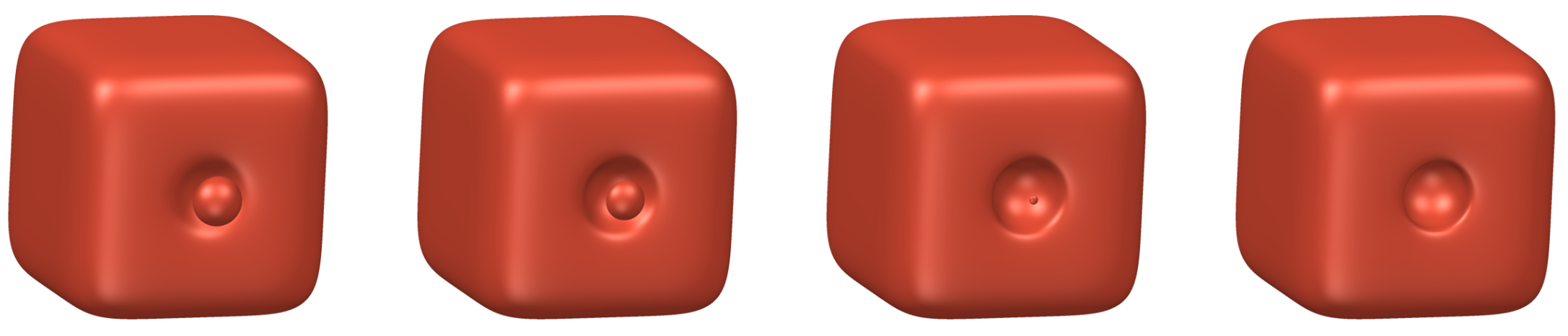
Subtractive shape composition means we interactively add negative primitives to an existing $\Pi$ -surface, as shown in Figure 7. Interestingly, the negative primitive used to create the concavity shrinks as it gets close to the existing object, and even vanishes at some point. This is a very useful feature because it eliminates undesired components in the final object; specifically, the negative sphere in Figure 7 is used to interactively create a concavity in one of the faces of a 3D cube. Notice how the sphere becomes smaller and smaller to a point at which it finally vanishes in the proximity of the cube.

2.4 Geometry Evaluation

The geometry evaluation (also known as boundary evaluation [RV85]) builds upon ray casting to solve two difficult problems in implicit surface modeling:

•

Rendering. We can immediately visualize the surface on screen with a significant realism and geometry fidelity, including singularities like apices, intersection curves, and the like, though without explicitly solving such singularities (i.e. the loci where the first derivatives vanish), as well as multi-component surfaces (see, for example, [RG06]).
•

Triangulation. The point sampling inherent to ray casting allows us to reconstruct the surface because we classify the surface points as either regular or singular using the gradient (i.e. first derivatives). Essentially, this problem consists in triangulating a point cloud whose points are samples of the surface (see, for example, [BMR+99, LHRS05, KBH06]). Note that the nearby points are associated with adjacent pixels on the screen so that the triangulation is more amenable to carry out than in standard surface reconstruction algorithms lacking information like normals or partial derivatives. Moreover, knowing the partial derivatives at such points, we can quickly identify singularities like apices, sharp features, self-intersections, and so forth. Summing up, we use a novel image-based surface reconstruction, though we also may use algorithms like those described by Skala et al. in [ČS04, ČS05, ČS07]. Obviously, after triangulating a surface, we no longer need ray casting for the purpose of the graphics output.

Thus, our renderer combines ray casting and triangulation approaches into a single renderer.

2.5 Molecular $\Pi$ -surfaces

Molecular modelling is an important application for $\Pi$ -surfaces. Knowing that each atom has a corresponding van der Waals (VDW) radius [Bon64][Bat01], a molecule can be seen as a set of overlapping spheres representing the atoms.

2.5.1 Molecular $\Pi$ -surface Formulation

The molecular surface $S$ of a molecule can be then described by the following $\Pi$ -surface:

S=\prod_{i=1}^{n}f_{i}-r

(2)

where

f_{i}=(x-x_{i})^{2}+(y-y_{i})^{2}+(z-z_{i})^{2}-{R_{i}}^{2}

(3)

represents the spherical surface of the $i$ -th atom of radius $R_{i}$ and center $(x_{i},y_{i},z_{i})$ . This formulation is in contrast with the Gaussian $\Sigma$ -surface proposed by Blinn [Bli82] to represent molecular surfaces.

It is worthy noting that for $r>0$ , Equation 2 represents a smooth molecular surface, so there is no need to use ray casting to sample the surface. Instead, we can directly triangulate the surface on-the-fly using triangulation algorithms as those described in [RG06, RQG09, DG11, DG15, DNJG17].

2.5.2 Examples of Molecular $\Pi$ -surfaces

Let us now see how to model the molecular structures of two real drugs using $\Pi$ -surfaces: (a) formic acid and (b) acetic acid.

Formic acid. This drug occurs naturally and is present in the venom of bees and ant stings. Using the atomic structure obtained from the DrugBank and the VDW radii from [Bat01] (1.52 Å for oxygen and 1.70 Å for carbon), the spheres have the following center points and radii:

c_{1}=(2.310,-1.334,0.000),R_{1}=1.52;

c_{2}=(3.644,-2.104,0.000),R_{2}=1.70;

c_{3}=(4.977,-1.334,0.000),R_{3}=1.52.

Then, using Equation 2 (with $r=1$ ) we obtain the $\Pi$ -surface that represents the formic acid molecule as follows:

	$\displaystyle S=((x-2.310)^{2}+(y+1.334)^{2}+z^{2}-1.52^{2})\cdot$
	$\displaystyle((x-3.644)^{2}+(y+2.104)^{2}+z^{2}-1.70^{2})\cdot$
	$\displaystyle((x-4.977)^{2}+(y+1.334)^{2}+z^{2}-1.52^{2})-1$

The formic acid $\Pi$ -surface is shown in Figure 8 (c).

Acetic acid. This drug results from the oxidation of ethanol and destructive distillation of wood. As seen in the previous example, the center points and radii of its atoms are as follows:

c_{1}=(24.214,-24.150,0.000),R_{1}=1.70;

c_{2}=(25.548,-23.380,0.000),R_{2}=1.70;

c_{3}=(26.881,-24.150,0.000),R_{3}=1.52;

c_{4}=(25.548,-21.840,0.000),R_{4}=1.52

Then, using Equation 2 (with $r=1$ ), we obtain the algebraic surface that represents the acetic acid molecule as follows:

	$\displaystyle S=((x-24.214)^{2}+(y+24.150)^{2}+z^{2}-1.70^{2})\cdot$
	$\displaystyle((x-25.548)^{2}+(y+23.380)^{2}+z^{2}-1.70^{2})\cdot$
	$\displaystyle((x-26.881)^{2}+(y+24.150)^{2}+z^{2}-1.52^{2})\cdot$
	$\displaystyle((x-25.548)^{2}+(y+21.840)^{2}+z^{2}-1.52^{2})-1$

The acetic acid $\Pi$ -surface is depicted in Figure 9 (c).

The Molecular $\Pi$ -surface formulation can also be used, for the sake of simplification, to model the four nucleotides (adenine, cytosine, guanine and thymine) used as DNA building blocks in [RG12, RG14, RG15], replacing the Gaussian $\Sigma$ -surface model.

3 Conclusions and Future Work

This paper presents a new general method to model complex 3D objects as the product of algebraic functions representing simpler implicit surface primitives. The resulting surfaces are here called $\Pi$ -surfaces. Unlike traditional methods used in implicit modeling, this new method is not based on a sum of specific distance functions. Instead, the 3D objects are built upon a product of algebraic functions representing arbitrary implicit surfaces such as spheres, ellipsoids, and tori. This new approach allows us to interactively perform controlled deformations on the object shape both locally and globally. Two possible applications are proposed for this new model: constructive building of 3D objects and molecular surfaces modeling. As future work, and knowing that an increase in the number of primitives might generate higher degree algebraic surfaces, it is our intention to develop some strategies to overcome possible limitations that may occur in these cases. As a final remark, we believe that this new method is an important contribution for the geometric modeling research field.

4 Acknowledgements

This research has been partially supported by the Portuguese Research Council (Fundação para a Ciência e Tecnologia), under the FCT Project UID/EEA/50008/2019. We are also grateful to reviewers for their suggestions to improve this paper.

REFERENCES

[Baj88] Chandrajit L. Bajaj. Geometric modeling with algebraic surfaces. In Proceedings of the 3rd IMA Conference on the Mathematics of Surfaces, Keble College, Oxford, September 19-21, 1988, pages 3–48, 1988.
[Bat01] S.S. Batsanov. Van der Waals radii of elements. Inorganic Materials, 37(9):871–885, 2001.
[Bed92] Sanjeev Bedi. Surface design using functional blending. Computer-Aided Design, 24:505–511, 09 1992.
[BGA04] Aurélien Barbier, Eric Galin, and Samir Akkouche. Complex skeletal implicit surfaces with levels of detail. Journal of WSCG, 12(1-3), 2004.
[Bli82] James F. Blinn. A generalization of algebraic surface drawing. In SIGGRAPH ’82: Proceedings of the 9th Annual Conference on Computer Graphics and Interactive Techniques, page 273, New York, NY, USA, 1982. ACM.
[BMR⁺99] F. Bernardini, J. Mittleman, H. Rushmeier, C. Silva, and G. Taubin. The ball-pivoting algorithm for surface reconstruction. IEEE Transactions on Visualization and Computer Graphics, 5(4):349–359, 1999.
[Bon64] A. Bondi. Van der Waals Volumes and Radii. J Phys Chem, 68(3):441–451, 1964.
[BX97] Chandrajit L. Bajaj and Guoliang Xu. Spline approximations of real algebraic surfaces. Journal of Symbolic Computation, 23(2-3):315–333, 1997.
[CCD00] F.L. Chen, C.S. Chen, and J.S. Deng. Blending pipe surfaces with piecewise algebraic surfaces. Chinese Journal of Computers, 23(9):911–916, 2000.
[ČS04] Martin Čermák and Václav Skala. Curvature dependent polygonization by the edge spinning. In Antonio Laganá, Marina L. Gavrilova, Vipin Kumar, Youngsong Mun, C. J. Kenneth Tan, and Osvaldo Gervasi, editors, Computational Science and Its Applications – ICCSA 2004, pages 325–334, Berlin, Heidelberg, 2004. Springer Berlin Heidelberg.
[ČS05] Martin Čermák and Vaclav Skala. Polygonization of implicit surfaces with sharp features by edge-spinning. The Visual Computer, 21:252–264, 05 2005.
[ČS07] Martin Čermák and Vaclav Skala. Polygonisation of disjoint implicit surfaces by the adaptive edge spinning algorithm of implicit objects. Int. J. Comput. Sci. Eng., 3(1):45–52, July 2007.
[DG11] Sérgio E.D. Dias and Abel J.P. Gomes. Graphics processing unit-based triangulations of blinn molecular surfaces. Concurrency and Computation: Practice and Experience, 23(17):2280–2291, 2011.
[DG15] Sérgio E.D. Dias and Abel J.P. Gomes. Triangulating molecular surfaces over a lan of gpu-enabled computers. Parallel Computing, 42:35–47, February 2015.
[DNJG17] Sérgio E.D. Dias, Quoc Trong Nguyen, Joaquim Jorge, and Abel J.P. Gomes. Multi-gpu-based detection of protein cavities using critical points. Future Generation Computer Systems, 67:430–440, February 2017.
[Gom03] Abel Gomes. A concise b-rep data structure for stratified subanalytic objects. In Proceedings of the Eurographics/ACM SIGGRAPH Symposium on Geometry Processing (SGP’03), Aachen, Germany, June 23-25, pages 83–93. Eurographics Association, 2003.
[GRM99] Abel Gomes, Chris Reade, and Alan Middleditch. A mathematical model for boundary representations of n-dimensional geometric objects. In Proceedings of the 5th Symposium on Solid Modeling and Applications (SPM’99), Ann Arbor, Michigan, USA, June 8-11, pages 270–277. ACM Press, 1999.
[GVJ⁺09] Abel Gomes, Irina Voiculescu, Joaquim Jorge, Brian Wyvill, and Callum Galbraith. Implicit Curves and Surfaces: Mathematics, Data Structures and Algorithms. Springer Publishing Company, Inc., 1st edition, 2009.
[HH85] C. Hoffmann and J. Hopcroft. Automatic surface generations in computer aided design. The Visual Computer, 1(2):92–100, August 1985.
[KBH06] Michael Kazhdan, Matthew Bolitho, and Hugues Hoppe. Poisson surface reconstruction. In Proceedings of the 4th Eurographics Symposium on Geometry Processing (SGP’06), Cagliari, Sardinia, Italy, June 26-28, pages 61–70, Aire-la-Ville, Switzerland, Switzerland, 2006. Eurographics Association.
[LHRS05] Florian Levet, Julien Hadim, Patrick Reuter, and Christophe Schlick. Anisotropic sampling for differential point rendering of implicit surfaces. In WSCG The 13th International Conference in Central Europe on Computer Graphics, Visualization and Computer Vision. UNION Agency - Science Press, Plzen, Czech Republic, 2005.
[LPP06] S. Lazard, L. M. Peñaranda, and S. Petitjean. Intersecting quadrics: an efficient and exact implementation. Computational Geometry: Theory and Applications, 35(1-2):74–99, 2006.
[Mur91] Shigeru Muraki. Volumetric shape description of range data using “blobby model”. SIGGRAPH Computer Graphics, 25(4):227–235, July 1991.
[NHK⁺85] Hiromitsu Nishimura, Masashi Hirai, Tsuyoshi Kawai, Tory Kawata, Isao Shirakawa, and Kengo Omura. Object modelling by distribution function and a method of image generation. Transactions of the IEICE Japan, J68-D(4):718–725, 1985.
[PK89] Markus Pilz and Hussein Kamel. Creation and boundary evaluation of CSG-models. Engineering with Computers, 5(2):105–118, 1989.
[RG06] Adriano N. Raposo and Abel J.P. Gomes. Polygonization of multi-component non-manifold implicit surfaces through a symbolic-numerical continuation algorithm. In Proceedings of the 4th International Conference on Computer Graphics and Interactive Techniques in Australasia and Southeast Asia (GRAPHITE’06), Kuala Lumpur, Malaysia, November 29 - December 02, pages 399–406, New York, NY, USA, 2006. ACM.
[RG12] Adriano N. Raposo and Abel J. P. Gomes. 3D molecular assembling of B-DNA sequences using nucleotides as building blocks. Graph. Models, 74(4):244–254, July 2012.
[RG14] Adriano N. Raposo and Abel J.P. Gomes. Efficient deformation algorithm for plasmid DNA simulations. BMC Bioinformatics, 15:301, Sep 2014.
[RG15] Adriano N. Raposo and Abel J. P. Gomes. isDNA: A tool for real-time visualization of plasmid DNA monte-carlo simulations in 3D. In Bioinformatics and Biomedical Engineering, pages 566–577. Springer International Publishing, 2015.
[RQG09] Adriano N. Raposo, J. Queiroz, and Abel J.P. Gomes. Triangulation of molecular surfaces using an isosurface continuation algorithm. In Proceedings of the 2009 International Conference on Computational Science and Its Applications, ICCSA ’09, pages 145–153. IEEE Computer Society, 2009.
[RV85] Aristides Requicha and Herbert Voelcker. Boolean operations in solid modeling: Boundary evaluation and merging algorithm. Proceedings of the IEEE, 73(1):30–43, 1985.
[War89] J. Warren. Blending algebraic surfaces. ACM Transactions on Graphics, 8(4):263–278, 1989.
[WMW86] Geoff Wyvill, Craig McPheeters, and Brian Wyvill. Data structure for soft objects. The Visual Computer, 2(4):227–234, Aug 1986.
[WZ00] T. R. Wu and Y. S. Zhou. On blending of several quadratic algebraic surfaces. Computer Aided Geometric Design, 17:759–766, 2000.

Π\Pi-surfaces: products of implicit surfaces towards constructive composition of 3D objects