Classical simulation of linear optics subject to nonuniform losses
Abstract
We present a comprehensive study of the impact of non-uniform, i.e. path-dependent, photonic losses on the computational complexity of linear-optical processes. Our main result states that, if each beam splitter in a network induces some loss probability, non-uniform network designs cannot circumvent the efficient classical simulations based on losses.
To achieve our result we obtain new intermediate results that can be of independent interest. First we show that, for any network of lossy beam-splitters, it is possible to extract a layer of non-uniform losses that depends on the network geometry. We prove that, for every input mode of the network it is possible to commute layers of losses to the input, where is the length of the shortest path connecting the th input to any output. We then extend a recent classical simulation algorithm due to P. Clifford and R. Clifford to allow for arbitrary -photon input Fock states (i.e. to include collision states). Consequently, we identify two types of input states where boson sampling becomes classically simulable: (A) when input photons occupy a constant number of input modes; (B) when all but photons are concentrated on a single input mode, while an additional modes contain one photon each.
1 Introduction and relation to previous works
The recent paradigm of quantum computational advantage (or supremacy), is regarded as a promising route towards demonstrating that quantum computers are more powerful than their classical counterparts [1]. Although the systems used in this approach are not expected to be universal for quantum computation, and are often not known to perform explicitly useful tasks, they allow us to test quantum mechanics in the limit of high computational complexity. The pursuit of a near-term demonstration of quantum superiority is also aligned with the overarching goals of the field of quantum computing, as it pushes the development of technologies that will undoubtedly be necessary for scalable universal quantum computers, and allows us to better understand the effects of real-world imperfections in intermediate-size quantum systems.
One candidate for demonstrating quantum advantage is nonadaptive linear optics, or boson sampling [2]. In this model, an -photon -mode Fock state evolves according to a passive -mode linear-optical transformation and is subsequently measured by particle-number resolving detectors [see fig. 1(a)]. This physical process leads to a probability distribution . The seminal contribution of [2] was to show that, subject to certain complexity-theoretic conjectures, for generic transformations it is hard for a classical computer to generate samples from a distribution suitably close to . Besides being an elegant and physically-motivated computational model and, arguably, the first proposal of quantum supremacy as we understand it today, boson sampling also benefits from the technology and expertise developed by the quantum optics community in the last decades [3].
Since the original proposal several small-scale boson sampling experiments have been reported [4, 5, 6, 7, 8, 9, 10, 11, 12, 13, 14, 15], with state-of-the-art ranging up to five photons with near-deterministic quantum dot sources [12, 13, 14]. From the opposite end, there has also been intense activity in the development of classical simulation algorithms [16, 17, 18], and current supercomputers are expected to simulate 50-photon experiments without much difficulty [19, 17]. A more refined analysis of the complexity-theoretic arguments underpinning boson sampling has suggested 90 photons as a concrete milestone for the demonstration of quantum computational advantage [20].
Many technological and theoretical challenges remain that can undermine the scalability of boson sampling. Several sources of imperfection affect linear-optical experiments, and it is essential to understand which can be mitigated and which degrade the computational power of the model. This boundary between classical simulability and quantum advantage is an area of intense investigation, with losses in particular receiving most attention. In [21] it was shown that boson sampling retains its computational power if a constant number of photons is lost. In the other extreme, recent papers showed that lossy boson sampling can be efficiently simulated when less than photons are left [22, 23] for arbitrary interferometers, or even when a suitably high constant fraction of the photons is lost for typical Haar-random interferometers [24] (see also a recent follow-up [25]). Boson sampling has also been investigated under the effect of fabrication noise in the linear-optical components [26, 27], losses combined with dark counts [28], partial photon distinguishability [29], and Gaussian noise in the experimental data [30].
In this work we build on our previous findings of [23] and solve some of the open problems posed there. The main result of [23] stated that, when less than out of photons are left, it is possible to approximate a lossy boson sampling state by a state of distinguishable photons, which is known to be classically simulable. This approximation is done at the level of the input state, and holds for arbitrary linear-optical experiments. For this result to work, it was necessary to assume losses happen at the input–a reasonable assumption when the interferometer is balanced, but which might fail for unbalanced network geometries [31]. To justify this, in [23] we also showed it is possible to commute layers of mode-independent losses to the input of the network, where is the smallest number of beam splitters in any path connecting any input to any output. However, it is possible to construct a universal linear-optical transformation where [31], suggesting a possible route to circumvent the algorithm of [23].
Here, we extend the results of [23] in different directions, with the goal of adapting them for very unbalanced network geometries [31]. In particular, our main result is that an unbalanced network geometry cannot be used to circumvent classical simulation due to losses. Our intermediate results regarding the accumulation of losses in linear-optical networks and an extension of the algorithm for simulation of boson sampling [17] can be also be of independent interest to the quantum optics and quantum complexity theory communities.
The paper is organized as follows. First, in section 2 we give an informal overview of our results. Sections 3-6 contain formal statements and proofs of our main results. Finally, appendix A contains the technical details needed in the proof of theorem 2.
Note added. After completion of this work, the first experimental demonstration of quantum computational advantage was realised in a chip consisting of 53 superconducting qubits [32]. The experiment implemented random circuit sampling, which constitutes another paradigm for realising quantum computational superiority [33]. Around the same time, a boson sampling experiment with 20 photons occupying 60 optical modes was reported in [34].
Notation and main concepts. Throughout the paper we use the following notation. Given two positive-valued functions and , we write if and if . Likewise, if . Finally, when . By () we denote the largest (smallest) integer smaller (larger) or equal to . We denote the total number of particles by , the total number of modes by , and by the -element set . We alternatively refer to input modes as “bins”, whenever there are many photons initialized in that mode (accordingly, we refer to this situation as bunching or binning). We also refer to any state where more than one photon occupies the same mode as a collision state.
The Hilbert space of photonic states in modes is spanned by Fock states, characterized by a definite photon number in each optical mode . In what follows we denote Fock states by , where is a vector of occupation numbers. In the formalism of second quantization we write , where is the standard creation operator associated to bosonic mode and is the vacuum state. Passive linear optical transformations are associated with unitary matrices , which induce the transformation of modes . When this transformation is applied to input state the output probabilities are given by
| (1) |
where denotes the permanent of and is an matrix constructed according to the following prescription. We first construct an matrix by taking copies of the th column of , then construct an matrix by taking copies of the th row of . 11 1 The arguments for computational hardness of Boson sampling rely on the fact that computation of the permanent is a -hard problem. Importantly, however, a device implementing boson sampling does not, in general, have the power to accurately compute or estimate permanents that appear in Eq. (1).. Boson sampling can also be framed in the language of first quantization, which we briefly use (see e.g. [35] or the introductory section of [23] for the translation between the two descriptions).
2 Overview of main results
In this Section we give an informal summary of our main findings and discuss the relation to previous work.
Result 1: Extracting nonuniform losses from the network. We improve the procedure of [23] to commute losses to the input of a network. For simplicity, we make the following assumptions regarding losses. We assume that all losses happen within the network and are located at beam splitters, and that every beam splitter carries the same amount of loss. Although losses due to imperfect sources and detectors are experimentally important [14], they are in principle constant, whereas losses due to linear-optical elements dictate how overall transmissivity of the network scales as the experiments become more complex. Furthermore, the geometry of a network is the main source of loss non-uniformity which we wish to study. Experimentally, beam splitter losses are also relevant e.g. in integrated photonic devices, since waveguide bends required to build directional couplers can cause photons to leave in unguided modes [5]. We represent a lossy linear-optical network as in fig. 2(a).
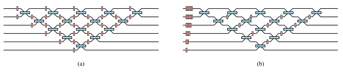
The main figure of merit for the result of [23] is the length of input-output paths inside a network, measured in the number of beam splitters a photon has to traverse along that path. Previously it was known that, if the shortest input-output path has length , we can rewrite the network in such a way that it has layers of mode-independent losses at the input. However this is not particularly useful for unbalanced networks such as that of Reck et al [31], depicted in fig. 2(a), as in that case we can only pull out one layer of uniform losses.
Our new result improves on this by showing how to extract nonuniform loss layers. More specifically, let be the shortest path between input and any output within some network. We show how to write an equivalent network that is preceded by a round of losses where input suffers the effect of consecutive loss elements. The precise formulation of this result can be found in theorem 1. Our proof is efficient and constructive, and works for networks of arbitrary geometry. The final result is illustrated in fig. 2(b) for the case of the network of Reck [31]. Overall, our result gives a more efficient description of the network where asymmetry is taken into account, and which we use to prove result 4 described later.
Result 2: Classical simulation of boson sampling with collision input states. It is well known that boson sampling is efficiently classically simulable if all photons are initialized in a single mode, i.e., input state . This follows from the fact that the permanent of a matrix of repeated columns can be computed trivially in linear time [2], or alternatively from the fact that if all photons are initialized in the same mode they behave as distinguishable particles [23]. Here we prove a stronger version of this result, by identifying two new types of input state which allow for efficient classical simulation of boson sampling [see fig. 1(b) and fig. 1(c)]. The first (type A) corresponds to photons concentrated in a constant number of input modes. The second (type B) is when all but photons are concentrated on a single input mode, while an additional modes contain one photon each.
Concretely, we provide a strong simulation of boson sampling (i.e. computing outcome probabilities) by showing how an expression for the permanent function from [36] can be computed efficiently for inputs of types A and B (though a similar scaling follows from an Appendix of [37]). We then generalize a result of [17] for weak classical simulation (i.e. producing samples from the correct distribution) to allow for bunched inputs, showing that it is efficient for inputs of types A and B. Our extension of the result of [17] is also based on a physical description of the state (via first quantization) rather than combinatorial considerations, and we believe it could make the original result more transparent for researchers with a stronger physics background. The technical formulation of this result can be found in theorem 2 and in corollary 1.
Besides giving us a new understanding of the regimes where efficient classical simulability of boson sampling is possible, and ruling out attempts at demonstrating a quantum advantage with highly concentrated bosonic input states, this result also serves as a nontrivial stepping stone towards result 3 described below.
Result 3: Classical simulation of lossy boson sampling with a few lossless modes. We improve the classical simulation algorithm of [23] by allowing the lossy boson sampling instance to be coupled to some lossless modes. Concretely, suppose that photons pass through a lossy channel in such a way that less than survive, and are then combined with up to photons input in modes that have perfect transmission. We show that the classical simulation based on the ideas similar those of [23] works for this setting as well. The technical formulation of this result can be found in theorem 3.
The classical simulation of [23] was based on approximating a lossy bosonic state by another state where photons effectively behave as distinguishable particles, then leveraging known results for classical simulation in that case [2]. Our new result is based on appending up to single-photon states to , and using this state to simulate the state obtained by also appending photons to . The state is a convex combination of states of type B so we can leverage result 2 above. The distance between the two states (and hence the error bound on the simulation) is the same as in [23], but the simulation is more costly due to the use of theorem 2. This result is also essential to prove result 4 that follows.
Result 4: Nonuniform losses do not avoid classical simulation. By combining results 1–3 we obtain our main result. Informally it states that the classical simulation algorithms of [23, 22] cannot be circumvented by the design of unbalanced networks such as that of Reck et al [31] (see theorem 4 for the formal statement). This was left as an open question in [23]. The idea was that, in an unbalanced network, there might be some input modes where losses are very mild, and the high chance of survival of these photons might break the assumptions behind the simulation algorithm in [23, 22]. Here we show that classical simulation remains possible as long as only inputs have small optical path to the output. Our result can be immediately applied to lossy interferometers with the geometry proposed in [31]. This closes one avenue for scaling up boson sampling experiments, but is also relevant for current experiments since this geometry is common in integrated-photonic implementations [10, 5].
In what follows we outline our argument for the simulability of the triangular construction of [31] [cf. fig. 2(b)]. This construction has the property that the shortest path from mode to any output has length (if we label modes starting from the lowest one). Suppose the input state we wish to simulate occupies the bottom modes in an attempt to avoid losses as much as possible. To simplify the argument, suppose now that the bottom modes are lossless (or include their loss channel as part of the network rather than the input state). By result 1 we can extract more than loss elements for all modes above mode . However, as discussed in [23], given a per-beam splitter loss parameter , there is always some such that, if an -photon state suffers rounds of losses, we expect less than photons to survive on average. Therefore, the input to the network is amenable to approximation by a convex combination of states of type B, as described in result 3, and so efficient classical simulation is possible.
3 Extracting nonuniform losses from a lossy network
Linear-optical networks are the natural implementation of general multimode interferometers. They are typically built by composition of simple few-mode transformations, often easier to realize in practice, which are then arranged in some network layout (see [31, 9] for the commonly used geometries, [38, 39, 40] for mathematical perspective, and [41] for the generalization to non-unitary transformations). At the same time, each small transformation also introduces some loss. The purpose of this Section is to provide an effective description of lossy linear-optical networks that takes into account their geometric properties.
Our focus is on losses induced by linear-optical elements within the circuit, such as beam-splitters, which determine how losses scale with the size of experiments. We disregard losses in detectors and sources, as well as uniform losses associated with free-space or waveguide propagation. These do not depend on the network layout and can be easily incorporated into our description as additional losses at the input of the network (alternatively, any path-dependent transmission loss can be incorporated into the nearest beam splitter). A loss channel that acts uniformly on modes is parameterized by a transmission probability , and its action on an -photon state can be written as:
| (2) |
where is the probability that out of particles remain. This is equivalent to adding an extra beam splitter that, with amplitude , diverts each photon into some inaccessible mode [see fig. 3(a)]. It can be easily shown that .

It is well-known that a layer of identical loss elements commutes with any linear-optical network acting only on the same modes. In fig. 3(b) this is represented for . This is the rationale for a standard assumption that losses happen at the input of a network, as it is usually assumed that they are approximately mode-independent. In practice, however, losses can also occur in nontrivial optical elements composing a network. In what follows, we assume for simplicity that each beam splitter carries two identical loss elements at its inputs. In [23] we showed the following. Given some linear-optical network built out of the building block of fig. 3(b), let be the smallest number of beam splitters that a photon has to traverse within the network starting from any input to reach any output. It is possible to rewrite this network as a different (possibly still containing some losses) linear-optical network preceded by uniform layers of loss elements. This formalized the assumption that losses happen at the input by basing it on a geometrical property of the network, namely the smallest number of loss elements that will affect any photon as it propagates inside it.
The above result works very well for symmetric networks, such as that of Clements et al [42], depicted in fig. 4(a), but not for unbalanced network such as the triangular decomposition of Reck et al [31], depicted in fig. 4(b) (often used in integrated photonics [10, 5]). For the construction of Reck et al specifically, the previous result only allows commuting a single layer of losses to the input. This led us to conjecture it might be possible to circumvent the efficient classical simulation of [23] by using purposely unbalanced networks. Motivated by this we now prove a stronger result that allows us to treat each mode individually. Namely we show that for, each input mode , it is possible to pull loss elements to the beginning of the network, where is the smallest number of beam splitters in any path between mode and any output mode.

Theorem 1.
Let be an -mode linear-optical network composed of beam splitters, each associated with a transmission probability . Let the length of a path connecting some input and output modes be the number of beam splitters that a photon encounters along that path. Let be the shortest path between input mode and any output mode. The quantum channel associated with the entire network can be decomposed as follows:
| (3) |
Here is a nonuniform loss channel described by , where is the transmission probability for mode , and is another (possibly still lossy) linear-optical network that can be described explicitly and efficiently (in the number of modes and beam splitters in the network).
Proof.
We assume without loss of generality that the network is arranged in layers, where each layer contains at most beam splitters acting on disjoint pairs of modes. Under our assumption that each beam splitter is preceded by one loss element in each of its inputs, the length of some input-output path corresponds to the number of loss elements the photon encounters in that path.
We prove the Theorem by iteratively applying the identity of fig. 3(b). We begin with the last layer in the network, and build it by progressively adding each previous layer one beam splitter at a time. At each step we commute losses through the new beam splitter to make sure the new network has a specific form.
Consider initially the more general situation of fig. 5(a). We have some linear-optical network . It is composed of a network , that can contain any number of beam splitters and loss elements distributed in an arbitrary manner, preceded by a layer of loss elements with transmissivity in mode . We add to the beginning of a new beam splitter, , acting on modes and (and two corresponding loss elements with transmissivity ). We cannot necessarily commute and through , as they may not be equal, but we can commute losses corresponding to the smallest of them. Suppose , and write . We can commute two loss elements through , leaving behind a loss element in mode . We are now left with the situation of fig. 5(b).
Let us now return to our network and apply the above procedure. Start with the last layer of beam splitters. Clearly it can be written in the form of of fig. 5(a). We now add each previous layer, one beam splitter at a time, always applying the argument of the previous paragraph and fig. 5. Suppose that, at step of this iteration, we have some intermediate network as in fig. 5(a). Suppose also that where is the length of the shortest path between input mode of and any output. In other words, we assume that at step the intermediate network satisfies the statement of our theorem.
Consider now the next beam splitter to be added to the network, , acting between modes and . By the reasoning of fig. 5 we can now commute loss elements through both modes of . The new network consisting of and has three properties:
- (i)
the shortest path starting from either input or has length ,
- (ii)
there are loss elements at both inputs modes and , and
- (iii)
the action of the network on modes other than and is unchanged.
Clearly the new network, , also satisfies the statement of our theorem. Therefore, by induction, this holds all the way until the network is complete. Furthermore, this procedure is constructive by also giving explicitly the form of . We conclude the proof by noting that the above scheme is also efficient, in the sense of requiring only polynomial effort in the number of modes and beam splitters in the network.
∎
Remark 1.
As stated above, our result can be easily extended to include losses in the preparation and measurement stages of the experiment. Indeed, let and be channels describing (possibly non-uniform) losses occurring during the state-preparation and readout phases respectively. The quantum channel describing the whole physical process is then given by . Combining this with (3) we get a decomposition
| (4) |
where and .
Remark 2.
Inspection of the proof of theorem 1 shows that the decomposition of Eq. (3) also holds in a network in which different optical elements induce different loss probabilities. In that case, it is still possible to write a decomposition similar to Eq. (3) where, for each input , we pull out a factor
where are all paths connecting input to some output, indexes all linear-optical elements connected to input , each with transmissivity , and the product is taken over all ’s in path . More explicitly, we pull out sufficient losses such that the final network has one completely lossless path from input to some output. To see how this follows from the proof of the Theorem, note two things about the procedure of fig. 5: (i) it does not require each beam splitter to have equal loss, and (ii) at every iterative step, it leaves one output port of lossless. Therefore, it will create one completely lossless path from each input to some output bu construction.
Finally we point out that, if each beam splitter has a different amount of loss, this might affect conclusions about finite-sized experiments drawn from our results, but it will not change any of our asymptotic conclusions.
4 Simulation of boson sampling with binned inputs
In this Section we describe two new types of input states for which boson sampling is easy to simulate classically. One of them (type B) will be used later in a classical simulation for optical networks with nonuniform losses. We start by providing a generalization of the algorithm by P. Clifford and R. Clifford [17]. This generalization, contrary to its predecessor, works for bunched input states, and similarly avoids an exponential cost in the number of modes . The proof of the following Theorem follows a similar reasoning to that of [17]. The main difference lays in the extensive usage of the first quantization formalism, which makes it easier to perform the necessary combinatorics and, in our opinion, can make the algorithm more approachable for physicists.
Theorem 2 (Generalization of the algorithm of P. Clifford and R. Clifford to collision input states).
Consider an -photon, -mode boson sampling instance described by linear optical transformation and an input state . We do not assume . There exists a classical algorithm that generates a sample from the output probability distribution in time upper bounded by
| (5) |
where is the number of nonzero ’s. Moreover, the algorithm also outputs the probability corresponding to the sampled outcome.
Proof.
Let encode the input state with photons in mode such that . Define similar quantities for the output state . In what follows the initial configuration of photons is fixed while denote the possible outcomes of boson sampling experiment.
We split the proof into two parts. First, we recall the results of [36] to give bounds on the computation cost on individual probability amplitudes . Then we show, by generalizing the ideas from [17], how to sample from the output probability distribution by sampling the evolution of the individual particles one at the time, sidestepping the need to compute exponentially many individual probabilities.
We start by reviewing results of [36]. According to Eq. (1), the probability of some outcome is proportional to . This permanent can be expanded as follows:
| (6) |
where . Let us compute the cost of calculating the permanent in this manner. First note there are terms for each of the sums. For each term in that multiple sum we need to compute
The product requires computing terms (since those with do not contribute), and the sum has terms for similar reasons (i.e., if then as well). Since the absolute value of the permanent is invariant under exchanging and , computing according to the expansion in eq. 6 has a runtime of
| (7) |
For the second part of the proof, we move from the usual notation of second quantization (or mode occupation lists) where a state is represented as a list of occupation numbers [i.e. ], to a notation native to first quantization (or mode assignment lists). In this notation states are represented by multisets of elements in , which we represent as tuples written in nondecreasing order, i.e. . Each represents in which mode photons is. Mapping back to the previous notation is easy: just identify as the multiplicity of mode in . More details on the mapping between these descriptions can be found in appendix A.
The first step in constructing the sampling algorithm is to enlarge the sample space. Instead of sampling output states as multisets , we can sample a tuple and rewrite it in nondecreasing order to obtain the output . It is easy to show [see Eq.(27) in appendix A] that sampling from the distribution
| (8) |
and then reordering is equivalent to sampling from the correct boson sampling distribution. Notice that, in the above equation, we have expanded the sample space for the outputs but not for the inputs, since those are fixed (and of type A or B). We have also defined in a similar spirit to just above eq. 6, but now for each in we take row of . The claim that sampling from eq. 8 is equivalent to sampling from the correct distribution follows from the fact that the permanent is invariant under permutations of rows and columns, and so it is equal for all ’s that, when reordered, lead to the same .
The second step is to find the marginal probability mass function (pmf) of leading subsequences of . The combinatorial factors that appear in the expression for this pmf make it cumbersome to write explicitly. In appendix A we show how to compute these marginal pmfs, and show that they have two properties crucial for the simulation algorithm (which they share with the corresponding pmfs for no-collision inputs, i.e. Lemma 1 in [17]):
- (i)
the probability of outcome , for , is the sum over probabilities corresponding to all inputs consistent with choosing photons from the actual -photon input state , and
- (ii)
each term in that sum corresponds to an input with the same binning structure as .
Therefore, if for some input the permanents can be efficiently computed, then the same is true for individual marginal probabilities of the distribution .
We now describe the sampling algorithm. This is done by sampling the marginal distributions one at a time. That is, we use the chain rule for conditional probabilities to write
| (9) |
It is easy to see that, for fixed , sampling according to is equivalent to sampling it according to (unnormalized) weights , and similarly for the subsequent ’s. Therefore, the above expression allows us to sample the elements of in order, one at a time, by computing the corresponding marginal probabilities.
All that remains is to determine the running time necessary to generate a sample with the above procedure. There are steps. In step , there are probabilities we need to compute according to the possible values of (recall that to are fixed by previous steps). Each probability requires computing some number of permanents, as per property (ii) above [cf. the discussion after eq. 29 in appendix A]. Each of these permanents can be computed in time equal to at most
| (10) |
This follows from Eq. (7), and details can be found in appendix B. Therefore, the runtime of the algorithm can be upper bounded by
where is the number of -photon configurations that can result by removing photons from the initial configuration [see discussion preceding Eq.(30)]. Finally, note that , which concludes the proof. ∎
A straightforward inspection of Eq. (5) shows that, for the standard collision-free boson sampling input (i.e. ), our algorithm remains with an exponential (in ) running time. However, using this formula we can identify two new families of input states for which boson sampling can be efficiently simulated classically.
Corollary 1 (Efficient classical simulation of boson sampling for certain classes of unbalanced inputs).
Consider the following two types of input states:
- A
: A Fock state with photons distributed arbitrarily in O different input modes (or bins).
- B
: A Fock state with photons distributed in = bins such that modes contain a single photon and all remaining photons are in the th mode.
Then, from (5) it follows that there exists an efficient classical algorithm to simulate the corresponding instances of boson sampling. The runtimes of this algorithm for inputs of type A and B are, respectively,
If and are constants, and in the standard boson sampling assumption that O, we have
Note that is not a consequence only of having bins. To see this, suppose we have bins with photons each. In this case the running time for the computation of a single permanent according to Eq. (10) is
| (11) |
which is super-polynomial in . Therefore, the restriction that inputs of type B have most photons starting in a single mode is important.
We finally remark that types A and B of inputs states do not exhaust all the cases for which the reasoning given in the proof of Theorem 2 gives an efficient classical sampling algorithm. In particular, it was pointed out to us by Alex Moylett that the following class of input states, interpolating between types A and B, is also classically simulable:
- C
: An -photon Fock state with photons distributed in input modes, where and . Moreover, photons located in modes “A” are distributed arbitrarily and remaining photons follow the distribution specified in the definition of input of type B.
5 Efficient simulation of lossy boson sampling with some lossless inputs
We now combine the ideas underlying the classical simulation of lossy boson sampling from [23] with the results from the preceding section to expand the known scenarios for which boson sampling becomes classically simulable. We begin by recalling the notion of total variation distance—the figure of merit typically used to assess the accuracy of boson sampling [2]. The total variation distance between probability distributions and is given by
| (12) |
Importantly, the total variation distance between probabilities and generated by measuring two quantum states and , respectively, with the same measurement is always upper bounded by the trace distance between and ,
| (13) |
We are now ready to formally state our result.
Theorem 3 (Classical simulation of lossy states when photons in some modes are not lost).
Consider an -mode -photon input state
| (14) |
and a linear-optical transformation , where is some (perhaps lossy) linear optical transformation, and is a pure loss channel such that the first modes have zero loss, while the remaining modes have transmission probability , i.e. we have
| (15) |
Let be the probability distribution obtained by measuring the output state with particle-number measurements. Then, provided , for any there exists a (weakly) classically simulable distribution which satisfies
| (16) |
Consequently, if , the error incurred in approximating with the (classically easy) distribution goes to as the number of particles tends to infinity.
Proof sketch.
The proof generalizes the main idea from [23] where the classical simulation of lossy linear optics was based on approximating the lossy bosonic state on particles by particle-separable states, i.e. states of the form
| (17) |
Importantly, state can be generated from by application of linear-optical transformation .
The lossy state considered in [23] was of the form , where is the channel that describes uniform losses [see Eq.(2)] and is a standard boson sampling input state on particles. It was shown that there exists a particle-separable state and a probability distribution that can be sampled efficiently, and such that the trace distance to the target state is upper bounded by
| (18) |
From the above and the fact that boson sampling with input states can be simulated classically it follows that any linear-optical process applied to and terminating with particle-number measurements can also be (weakly) simulated classically within total variation distance .
Here we generalize the above argument to the situation at hand. The key difference is that, as the (partially) lossy input state, we take the state for which no particles are lost in the first modes. We can approximate by
| (19) |
where, in contrast to Eq. (17), states entering in the above convex decomposition are of the type , where and is a suitable linear optical unitary transformation that acts as the identity on the first optical modes. If , states of type lead to classically easy boson sampling instances (they belong to type B appearing in Theorem 2). Repeating the considerations that led to Eq.(18) we conclude it is possible to choose a distribution which can be sampled efficiently and for which we have
| (20) |
By the assumptions stated above, sampling from can be done efficiently, which concludes the proof. ∎
6 Classical simulation of linear optics in unbalanced lossy networks
In this Section we combine results from Theorems 1 and 3 to show that, for arbitrary lossy linear networks, boson sampling becomes classically simulable provided there are at most O() input modes for which the input-output paths are short.
Theorem 4 (Classical simulation in unbalanced lossy networks).
Consider an -mode lossy optical linear network acting on the standard input -photon state of the form
| (21) |
Assume every beam splitter introduces losses, characterized by transmissivity , on the modes on which it acts. Moreover, assume that at most inputs are such that their shortest input-output path has length smaller than for some suitable constant . Then there exists a classical algorithm to sample from a that approximates the target output distribution , obtained by evolving the input state through network , to accuracy
| (22) |
where . In particular, if , then as the number of photons increase.
Proof.
The result follows directly from Theorems 1 and 3. First, note that at most input modes have their shortest input-output path of length . Then, by Theorem 1, we can extract from the network a layer of nonuniform losses that, up to relabeling of modes, is of the form
| (23) |
Next, note that assumptions of Theorem 3 are met since and the vector of losses from Eq. (23) directly corresponds to Eq. (15). By directly invoking of Theorem 3 we obtain Eq. (22), which concludes the proof. ∎
Example 1 (Triangular decomposition of linear-optical networks [31]).
Consider the standard construction of linear-optical networks given in Fig. 2. Assume that every beam splitter in the network is lossy. The number of beam-splitters photons need to cross, as they propagate from input (counting from the bottom of the network) scales linearly with . Therefore, a lossy network in this geometry satisfies the assumptions of Theorem 4 and the corresponding boson sampling instance can be simulated as described in the statement of the Theorem.
7 Conclusions and outlook
We presented a comprehensive study of the effect of nonuniform losses on classical simulability of boson sampling. Our main conclusion is that linear-optical networks for which losses exhibit high degree of non-uniformity cannot evade a classical simulation strategies based on ideas from [22, 23]. Our main contributions are twofold. First, in theorem 1 we established the quantitative relation between the geometric properties of lossy networks and the amount of losses that can be pulled-out to the input of the network. Second, in theorem 4 we provided sufficient conditions for effective classical simulability of of boson sampling subject to nonuniform losses (that can result, for example, from the complicated network structure). To establish the second result we extended the classical simulation algorithm from [17] to instances of boson sampling with binned inputs. This allowed us to identify two classes of input states for which the simulation of boson sampling becomes efficient: (A) when input photons occupy a constant number of input modes; (B) when all but photons are concentrated on a single input mode, while an additional modes contain one photon each.
We believe that our results can help in understanding which linear-optical designs can offer scalable platforms for demonstration of quantum advantage based on boson sampling. Moreover, the classical simulation techniques presented here can be leveraged to benchmark the performance of photonic networks with complicated input states in the near future. We would like to conclude by stating a number of interesting open questions.
First, in a recent work [24] Renema et al. proved that, for typical (i.e. Haar-random) linear-optical interferometers , boson sampling can be classically simulated if only a constant fraction of input photons are lost and every optical mode suffers from identical losses. The technique used in [24] was based on approximating the lossy output probability distributions by distributions originating from interference of partially distinguishable photons (with increasing degree of indistinguishability). It is an interesting question whether input states of type A or type B can be used to obtain similar results for generic multi-mode interferometers.
Another interesting question is what are the consequences of our result for Gaussian boson sampling [43], a variant of boson sampling that uses squeezed Gaussian states as input. A recent work [44] studied under which conditions lossy Gaussian boson sampling becomes easy to simulate. We conjecture that our results from section 4 can be adapted to the case of Gaussian boson sampling to prove, for example, that it is also classically simulable if the squeezed states are inputs only in O. We also conjecture that our results of section 6 can be adapted to show that the conclusions of [44] also hold for unbalanced networks (there, the authors made the standard assumption of uniform losses).
Lastly, nonuniform losses clearly seem to undermine the quantum features of nonclassical states. It is natural to explore the consequences of our results regarding extraction of nonuniform losses from a lossy network (theorem 1) for the nonclassical features of quantum states generated by such networks [45].
Acknowledgements.
We thank Michał Horodecki for interesting and fruitful discussions. M. O. acknowledges the financial support by TEAM-NET project (contract no. POIR.04.04.00-00-17C1/18-00). D. J. B. acknowledges funding from Instituto Nacional de Ciência e Tecnologia de Informação Quântica (INCT-IQ/CNPq).References
- Harrow and Montanaro [2017] A. Harrow and A. Montanaro. Quantum computational supremacy. Nature, 549:203–209, 2017. doi: 10.1038/nature23458.
- Aaronson and Arkhipov [2013] S. Aaronson and A. Arkhipov. The computational complexity of linear optics. Theory of Computing, 4:143–252, 2013. doi: 10.4086/toc.2013.v009a004.
- Brod et al. [2019] D. J. Brod, E. F. Galvão, A. Crespi, R. Osellame, N. Spagnolo, and F. Sciarrino. Photonic implementation of boson sampling: a review. Advanced Photonics, 1(3):1–14, 2019. doi: 10.1117/1.AP.1.3.034001.
- Broome et al. [2013] M. A. Broome, A. Fedrizzi, S. Rahimi-Keshari, J. Dove, S. Aaronson, T. C. Ralph, and A. G. White. Photonic Boson Sampling in a tunable circuit. Science, 339(6121):794, 2013. doi: 10.1126/science.1231440.
- Crespi et al. [2013] A. Crespi, R. Osellame, R. Ramponi, D. J. Brod, E. F. Galvão, N. Spagnolo, C. Vitelli, E. Maiorino, P. Mataloni, and F. Sciarrino. Integrated multimode interferometers with arbitrary designs for photonic Boson Sampling. Nat. Photon., 7(7):545–549, 2013. doi: 10.1038/nphoton.2013.112.
- Spring et al. [2013] J. B. Spring, B. J. Metcalf, P. C. Humphreys, W. S. Kolthammer, X.-M. Jin, M. Barbieri, A. Datta, N. Thomas-Peter, N. K. Langford, D. Kundys, J. C. Gates, B. J. Smith, P. G. R. Smith, and I. A. Walmsley. Boson Sampling on a Photonic Chip. Science, 339(6121):798, 2013. doi: 10.1126/science.1231692.
- Tillmann et al. [2013] M. Tillmann, B. Dakić, R. Heilmann, S. Nolte, A. Szameit, and P. Walther. Experimental Boson Sampling. Nat. Photon., 7(7):540–544, 2013. doi: 10.1038/nphoton.2013.102.
- Spagnolo et al. [2014] N. Spagnolo, C. Vitelli, M. Bentivegna, D. J. Brod, A. Crespi, F. Flamini, S. Giacomini, G. Milani, R. Ramponi, P. Mataloni, R. Osellame, E. F. Galvão, and F. Sciarrino. Experimental validation of photonic Boson Sampling. Nat. Photon., 8(8):615–620, 2014. doi: 10.1038/nphoton.2014.135.
- Carolan et al. [2014] J. Carolan, J. D. A. Meinecke, P. J. Shadbolt, N. J. Russell, N. Ismail, K. Wörhoff, T. Rudolph, M. G. Thompson, J. L. O’Brien, J. C. F. Matthews, and A. Laing. On the experimental verification of quantum complexity in linear optics. Nat. Photon., 8(8):621–626, 2014. doi: 10.1038/nphoton.2014.152.
- Carolan et al. [2015] J. Carolan, C. Harrold, C. Sparrow, E. Martín-López, N. J. Russell, J. W. Silverstone, P. J. Shadbolt, N. Matsuda, M. Oguma, M. Itoh, G. D. Marshall, M. G. Thompson, J. C. F. Matthews, T. Hashimoto, J. L. O’Brien, and A. Laing. Universal linear optics. Science, 349(6249):711, 2015. doi: 10.1126/science.aab3642.
- Bentivegna et al. [2015] M. Bentivegna, N. Spagnolo, C. Vitelli, F. Flamini, N. Viggianiello, L. Latmiral, P. Mataloni, D. J. Brod, E. F. Galvão, A. Crespi, R. Ramponi, R. Osellame, and F. Sciarrino. Experimental scattershot Boson Sampling. Science Advances, 1(3):e1400255, 2015. doi: 10.1126/sciadv.1400255.
- Loredo et al. [2017] J. C. Loredo, M. A. Broome, P. Hilaire, O. Gazzano, I. Sagnes, A. Lemaitre, M. P. Almeida, P. Senellart, and A. G. White. Boson Sampling with single-photon fock states from a bright solid-state source. Phys. Rev. Lett., 118:130503, 2017. doi: 10.1103/PhysRevLett.118.130503.
- He et al. [2017] Y. He, X. Ding, Z.-E. Su, H.-L. Huang, J. Qin, C. Wang, S. Unsleber, C. Chen, H. Wang, Y.-M. He, X.-L. Wang, W.-J. Zhang, S.-J. Chen, C. Schneider, M. Kamp, L.-X. You, Z. Wang, S. Höfling, Chao-Yang Lu, and Jian-Wei Pan. Time-bin-encoded Boson Sampling with a single-photon device. Phys. Rev. Lett., 118:190501, 2017. doi: 10.1103/PhysRevLett.118.190501.
- Wang et al. [2017] H. Wang, Y. He, Y.-H. Li, Z.-E. Su, B. Li, H.-L. Huang, X. Ding, M.-C. Chen, C. Liu, J. Qin, J.-P. Li, Y.-M. He, C. Schneider, M. Kamp, C.-Z. Peng, S. Höfling, C.-Y. Lu, and J.-W. Pan. High-efficiency multiphoton boson sampling. Nat. Photon., 11:361–365, 2017. doi: 10.1038/nphoton.2017.63.
- Wang et al. [2018a] H. Wang, W. Li, X. Jiang, Y.-M. He, Y.-H. Li, X. Ding, M.-C. Chen, J. Qin, C.-Z. Peng, C. Schneider, M. Kamp, W.-J. Zhang, H. Li, L.-X. You, Z. Wang, J. P. Dowling, S. Höfling, Chao-Yang Lu, and Jian-Wei Pan. Toward scalable Boson Sampling with photon loss. Phys. Rev. Lett., 120:230502, 2018a. doi: 10.1103/PhysRevLett.120.230502.
- Neville et al. [2017] A. Neville, C. Sparrow, R. Clifford, E. Johnston, P. M. Birchall, A. Montanaro, and A. Laing. Classical boson sampling algorithms with superior performance to near-term experiments. Nature Physics, 13:1153, 2017. doi: doi:10.1038/nphys4270.
- Clifford and Clifford [2018] P. Clifford and R. Clifford. The classical complexity of Boson Sampling. In Proceedings of the Twenty-Ninth Annual ACM-SIAM Symposium on Discrete Algorithms, page 146, 2018. doi: 10.1137/1.9781611975031.10.
- Roga and Takeoka [2019] W. Roga and M. Takeoka. Classical simulation of boson sampling with sparse output. 2019. arXiv:1904.05494.
- Wu et al. [2018] J. Wu, Y. Liu, B. Zhang, X. Jin, Y. Wang, H. Wang, and X. Yang. A benchmark test of boson sampling on Tianhe-2 supercomputer. National Science Review, 5:715, 2018. doi: 10.1093/nsr/nwy079.
- Dalzell et al. [2018] A. M. Dalzell, A. W. Harrow, D. E. Koh, and R. L. La Placa. How many qubits are needed for quantum computational supremacy? 2018. arXiv:1805.05224.
- Aaronson and Brod [2016] S. Aaronson and D. J. Brod. BosonSampling with lost photons. Phys. Rev. A, 93(1):012335, 2016. doi: 10.1103/PhysRevA.93.012335.
- García-Patrón et al. [2019] R. García-Patrón, J. J. Renema, and V. Shchesnovich. Simulating boson sampling in lossy architectures. Quantum, 3:169, 2019. doi: 10.22331/q-2019-08-05-169.
- Oszmaniec and Brod [2018] M. Oszmaniec and D. Brod. Classical simulation of photonic linear optics with lost particles. New Journal of Physics, 20(9):092002, 2018. doi: 10.1088/1367-2630/aadfa8.
- Renema et al. [2018] J. Renema, V. Shchesnovich, and R. García-Patrón. Classical simulability of noisy boson sampling. 2018. arXiv:1809.01953.
- Moylett et al. [2019] A. E. Moylett, R. García-Patrón, J. Renema, and P. Turner. Classically simulating near-term partially-distinguishable and lossy boson sampling. Quantum Science and Technology, 5(1):015001, 2019. doi: 10.1088/2058-9565/ab5555.
- Arkhipov [2015] A. Arkhipov. BosonSampling is robust against small errors in the network matrix. Phys. Rev. A, 92:062326, 2015. doi: 10.1103/PhysRevA.92.062326.
- Leverrier and García-Patrón [2014] A. Leverrier and R. García-Patrón. Analysis of circuit imperfections in BosonSampling. Quant. Inf. Comp., 15:489, 2014.
- Rahimi-Keshari et al. [2016] S. Rahimi-Keshari, T. C. Ralph, and C. M. Caves. Sufficient conditions for efficient classical simulation of quantum optics. Phys. Rev. X, 6(2):021039, 2016. doi: 10.1103/PhysRevX.6.021039.
- Renema et al. [2018] J. J. Renema, A. Menssen, W. R. Clements, G. Triginer, W. S. Kolthammer, and I. A. Walmsley. Efficient algorithm for boson sampling with partially distinguishable photons. Phys. Rev. Lett., 120:220502, 2018. doi: 10.1103/PhysRevLett.120.220502.
- Kalai and Kindler [2014] G. Kalai and G. Kindler. Gaussian Noise Sensitivity and BosonSampling. 2014. arXiv:1409.3093.
- Reck et al. [1994] M. Reck, A. Zeilinger, H. Bernstein, and P. Bertani. Experimental realization of any discrete unitary operator. Phys. Rev. Lett., 73:58, 1994. doi: 10.1103/PhysRevLett.73.58.
- Arute et al. [2019] F. Arute et al. Quantum supremacy using a programmable superconducting processor. Nature, 574(7779):505–510, 2019. doi: 10.1038/s41586-019-1666-5.
- Boixo et al. [2018] S. Boixo, S. Isakov, V. Smelyanskiy, R. Babbush, N. Ding, Z. Jiang, M. Bremner, J. Martinis, and H. Neven. Characterizing quantum supremacy in near-term devices. Nature Physics, 14(6):595–600, 2018. doi: 10.1038/s41567-018-0124-x.
- Wang et al. [2019] H. Wang, J. Qin, X. Ding, M.-C. Chen, S. Chen, X. You, Y.-M. He, X. Jiang, L. You, Z. Wang, C. Schneider, J. Renema, S. Höfling, C.-Y. Lu, and J.-W. Pan. Boson Sampling with 20 input photons and a 60-mode interferometer in a -dimensional Hilbert space. Phys. Rev. Lett., 123:250503, 2019. doi: 10.1103/PhysRevLett.123.250503.
- Moylett and Turner [2018] A. E. Moylett and P. S. Turner. Quantum simulation of partially distinguishable boson sampling. Phys. Rev. A, 97:062329, 2018. doi: 10.1103/PhysRevA.97.062329.
- Chin and Huh [2018] S. Chin and J. Huh. Generalized concurrence in boson sampling. Sci. Rep., 8:6101, 2018. doi: 10.1038/s41598.
- Shchesnovich [2013] V. S. Shchesnovich. Asymptotic evaluation of bosonic probability amplitudes in linear unitary networks in the case of large number of bosons. International Journal of Quantum Information, 11(05):1350045, 2013. doi: 10.1142/S0219749913500457.
- Bouland and Aaronson [2014] A. Bouland and S. Aaronson. Generation of universal linear optics by any beam splitter. Phys. Rev. A, 89:062316, 2014. doi: 10.1103/PhysRevA.89.062316.
- Sawicki [2016] A. Sawicki. Universality of beamsplitters. Quantum Inf. Comput., 16(3 and 4):0291–0312, 2016.
- Sawicki and Karnas [2017] A. Sawicki and K. Karnas. Universality of Single-Qudit Gates. Annales Henri Poincare, 18(11):3515–3552, 2017. doi: 10.1007/s00023-017-0604-z.
- Tischler et al. [2018] N. Tischler, C. Rockstuhl, and K. Słowik. Quantum optical realization of arbitrary linear transformations allowing for loss and gain. Phys. Rev. X, 8:021017, 2018. doi: 10.1103/PhysRevX.8.021017.
- Clements et al. [2016] W. R. Clements, P. C. Humphreys, B. J. Metcalf, W. S. Kolthammer, and I. A. Walmsley. Optimal design for universal multiport interferometers. Optica, 3(12):1460–1465, 2016. doi: 10.1364/OPTICA.3.001460.
- Hamilton et al. [2017] C. S. Hamilton, R. Kruse, L. Sansoni, S. Barkhofen, C. Silberhorn, and I. Jex. Gaussian Boson Sampling. Phys. Rev. Lett., 119:170501, 2017. doi: 10.1103/PhysRevLett.119.170501.
- Qi et al. [2020] H. Qi, D. J. Brod, N. Quesada, and R. García-Patrón. Regimes of classical simulability for noisy Gaussian boson sampling. Phys. Rev. Lett., 124:100502, 2020. doi: 10.1103/PhysRevLett.124.100502.
- Wang et al. [2018b] J. Wang, S. Paesani, Y. Ding, R. Santagati, P. Skrzypczyk, A. Salavrakos, J. Tura, R. Augusiak, L. Mančinska, D. Bacco, D. Bonneau, J. Silverstone, Q. Gong, A. Acín, K. Rottwitt, L. Oxenlowe, J. O’Brien, A. Laing, and M. Thompson. Multidimensional quantum entanglement with large-scale integrated optics. Science, 360(6386):285–291, 2018b. doi: 10.1126/science.aar7053.
Appendix A Marginal probabilities for partial photon outputs
In this Appendix, we show how to compute the marginal probabilities necessary for theorem 2. This generalizes Lemma 1 of [17] by allowing for collision inputs. The proof technique, however, is slightly different from that of [17], as we use the physical description of bosonic states via first quantization rather than combinatorial arguments. Therefore, we hope it might also make the original Lemma 1 of [17] more transparent for physicists.
Throughout this section we denote by an -boson, -mode Dicke state. We can write it as
| (24) |
where is the projector onto the -particle, -mode symmetric subspace, and . The state is such that is the number of times state appears in . Conversely, are the tuples as defined just above eq. 8.
Let now and be the (not necessarily collision-free) input and output states to a linear-optical circuit . In this formalism, we can write the corresponding transition probability as
| (25) |
where is the unitary transformation induced by in the -particle Hilbert space, i.e. . The above expression coincides with the standard definition of bosonic transition probabilities in terms of permanents of [2].
Expanding the output state as in eq. 24 we can write
| (26) |
where we have used the cyclic property of the trace and the fact that acts trivially on . Equation 26 is similar to eq. 8. It represents the fact that, due to the symmetries of the input state and the dynamics (or, equivalently, the symmetries of the permanent function), in order to sample from the output distribution over symmetric states (or multisets ) we can equivalently sample from the distribution over tuples given by
| (27) |
and reorder the outcome in nondecreasing manner.
Equation 27 gives us an expression for the full pmf over tuples . We now need to compute the marginal probabilities over leading subsequences of . To that end, let denote the subsequence of the first elements of , for , and let denote the remaining elements of the list over which we wish to marginalize. We can write the marginal pmf for that subsequence as
| (28) |
The sum inside the trace equals simply to the identity on the subspace of particles to . We can thus write the above as
| (29) |
where by we mean tracing over the last particles, and we have used the property that , as discussed in [23].
The result we need already follows from eq. 29. To see this note that is a convex combination over all -photon Dicke states compatible with choosing out of photons from input state i.e. states of the form
| (30) |
where and . The probability that a particular state appears in the decomposition of is proportional to the multinomial coefficient . Therefore, eq. 29 satisfies properties (i) and (ii) laid out above eq. 9. The fact that each probability in eq. 29 can be computed efficiently for input state of types A and B follows from the discussion in the proof of theorem 2.
Appendix B Upper bound on the cost of permanents involved in theorem 2
The maximal runtime associated to the computation of the individual permanent in the simulation algorithm given in the proof of theorem 2 can be computed via the following expression.
| (31) |
where
| (32) |
and the internal maximization is over all -photon input configurations that are compatible with with the initial state and over -photon outputs . Let us note that is a non-decreasing function of individual components of both inputs and . Therefore, for a specific number of particles we have . This concludes the proof of the upper bound from Eq.(10).