Tangle decompositions of alternating link complements
Abstract.
Decomposing knots and links into tangles is a useful technique for understanding their properties. The notion of prime tangles was introduced by Kirby and Lickorish in [3]; Lickorish proved [5] that by summing prime tangles one obtains a prime link. In a similar spirit, summing two prime alternating tangles will produce a prime alternating link, if summed correctly with respect to the alternating property. Given a prime alternating link, we seek to understand whether it can be decomposed into two prime tangles each of which is alternating. We refine results of Menasco and Thistlethwaite to show that if such a decomposition exists either it is visible in an alternating link diagram or the link is of a particular form, which we call a pseudo-Montesinos link.
1. Overview
We review some definitions and give an outline of the paper.
Let be a non-split prime alternating link in . A properly imbedded surface in the complement of is essential if it is incompressible, boundary incompressible and non-boundary parallel in .
A Conway sphere for is an essential 4-punctured sphere properly imbedded in the complement of with meridianal boundary components. We say that a Conway sphere splits into two 2-tangles, i.e., two 3-balls each of which contains two strands of . A 3-ball may also additionally contain components of disjoint from . Since is prime by hypotheses, the tangles on each side are prime. A 2-tangle in which the two strands are boundary parallel is called a rational tangle.
The notion of a prime tangle was suggested by Kirby and Lickorish in [3]. Lickorish shows in [5] that by summing prime tangles one obtains a prime link. Similarly, summing two prime alternating tangles produces a prime alternating link, if summed correctly with respect to the alternating property. Here, we look at the converse: given a prime alternating link diagram, can one determine whether it is a sum of two prime alternating tangles?
Menasco proved that a Conway sphere is realized in a reduced alternating diagram as either visible (represented by a PPPP curve in standard position) or hidden (two PSPS curves) in [6]. He also proved that two PSPS curves in a prime alternating diagram represent a 4-punctured sphere that is essential [7]. It is known how to determine whether a given PPPP curve (visible case) represents a 4-punctured sphere that is essential: see Menasco and Thislethwaite [9], and Thislethwaite [10]. All these facts together give a purely diagrammatic algorithm to determine whether the link has a decomposition into two prime tangles, though possibly not alternating.
We revisit the case of a “hidden” Conway sphere. We prove that such a sphere forces the presence of another visible Conway sphere right next to it, in the same diagram, unless the link is a pseudo-Montesinos link (Proposition 3.2). Pseudo-Montesinos links will be defined in Section 3 and are a subset of arborescent links [1]. This was not known before: rather, Thistlethwaite noted that a visible Conway sphere is always visible in an alternating diagram (i.e. if visible in one alternating diagram, then also visible in other alternating diagrams of the same link), and therefore a hidden one is always hidden [10]. We also prove that a pseudo-Montesinos link has no visible Conway spheres in any alternating diagram (Proposition 3.3 with corollaries). Our two results together yield that a decomposition into two prime alternating tangles can always be detected by looking at an alternating diagram (Theorem 3.1). In the final section we also show that for a closed braid , detecting prime alternating tangle decompositions takes an even easier form. Indeed, once the decomposing sphere is essential, it must be positioned in a special way with respect to (Proposition 4.1).
Our proofs mainly use two techniques. The first one is inherited from Menasco’s work: we use standard position, which helps to translate topology of a surface into combinatorics of curves and diagrams. The second component is a careful topological analysis of certain isotopies and strong isotopies of surfaces embedded in 3-manifolds.
The visibility of a prime alternating tangle decomposition (and of the genus-2 surfaces that yield an essential 4-punctured sphere after meridianal compressions) aligns with well-known results of Menasco, who noted that some of the basic topological properties of alternating link complements can be seen directly in reduced alternating link diagrams [6]. Among them is the property of a link being non-split (and respectively the presence of an essential genus-0 surface in the link complement), and the property of being prime (and the presence of an essential genus-1 surface).
2. Conway spheres and standard position
In this preliminary section, we recall Menasco’s techniques and a key lemma, as well some of the results of Thistlethwaite on rational tangles.
Let be a reduced alternating diagram of the link . Let be the projection sphere where lies except for perturbations at crossings. We review the notion of a surface in standard position (see Section 2 of [6]).
The link lies on a union of two spheres in , and , which agree with except in a bubble around each crossing. At the bubbles, and go over the top and bottom hemispheres respectively. We will denote by and the parts of lying above and below respectively.
Let be an essential surface properly embedded in the complement of such that every boundary component of is meridianal. If is closed, we meridianally compress it until no further meridianal compression is possible. Then consists of simple closed curves bounding disks of . Following Menasco’s technique, we encode such a curve of intersection by a word consisting of the letters and . The letter means intersects a strand of a link not at a crossing, i.e. has a meridianal boundary component there. The letter means intersects a crossing, i.e. passes between two strands of a crossing and is shaped as a saddle there. Fig.1 (1) depicts an example of a curve, projected on from (a fragment of a link diagram is pictured in grey). There are multiple ways to put a surface in standard position. If it is done so that the total number of ’s, ’s and the curves of is minimized, then is in complexity minimizing standard position.


A segment of from a crossing to an adjacent crossing will be called a edge.
Lemma 2.1.
Suppose is a closed essential 4-punctured sphere in the complement of a prime alternating non-split link , i.e., is a Conway sphere for . Then can be placed in standard position relative to so that
- (1)
intersects in either a single curve or in two curves.
- (2)
No curve passes through a saddle and then crosses an edge of adjacent to the saddle.
- (3)
No curve crosses an edge of twice consecutively.
Remark 2.2.
Menasco’s techniques found application in the work of Thistlethwaite on rational tangles [10], in which he describes precisely what an alternating diagram of a rational tangle looks like, as follows:
Start with a diagram of a 2-string tangle that has no crossings. Then surround this diagram by annuli, each annulus containing four arcs of the link diagram joining distinct boundary components of the annulus, and connected to the arcs in the neighboring annuli or the described 2-string tangle. Each annulus contains a single crossing between two of the arcs. See the comments after Corollary 3.2 in [10], as well as Fig.2 in [4] for an illustration. In particular, one can determine whether an alternating tangle diagram represents a rational tangle just by looking at the diagram.
3. Decomposition into two prime alternating tangles
A Montesinos link is a link obtained by taking a cyclic sum of a finite number of rational 2-tangles (see top of Fig.2 for an example; inside each circle insert a diagram of a rational tangle). We will often refer to these four tangles as sub-tangles, since together they may form larger tangles that we consider. Given a Montesinos link with four rational sub-tangles , we construct a pseudo-Montesinos link as follows: delete four strands, one each connecting to , to , to , and to . Then, following the pattern shown in the bottom of Fig.2, replace these strands with four strands, two between and and two between and . If the resulting diagram is reduced and alternating and each rational sub-tangle has at least one crossing we say that it is a standard diagram of an alternating pseudo-Montesinos link. Fig.3 (2) is an example of standard diagram of an alternating pseudo-Montesinos link.
In the terminology of Thistlethwaite ([10]), a visible 4-punctured sphere in an alternating diagram is one that appears in the plane of the diagram (after isotopy to standard position) represented by a curve. A hidden Conway sphere is one that is represented by two curves. We extend this to call any 2-tangle in visible if a curve intersects four arcs of such that all of lies on one side of , and the complement of (denote it by ) lies entirely on the other side of .
Our main theorem is the following:
Theorem 3.1.
Suppose is a prime alternating non-split link, is a reduced alternating diagram for , and there is an essential Conway sphere embedded in . Then a prime tangle decomposition of is visible in if and only if is not a standard diagram of an alternating pseudo-Montesinos link. Further, if is a standard diagram of an alternating pseudo-Montesinos link, then no prime tangle decomposition for is visible in any reduced alternating diagram for .
The rest of the section is devoted to the proof of Theorem 3.1 via a sequence of propositions.
Proposition 3.2.
Suppose is a prime alternating non-split link, is a reduced alternating diagram for , and there is an essential Conway sphere embedded in . Then either a prime tangle decomposition of is visible in , or is a standard diagram of an alternating pseudo-Montesinos link.
Proof.
Let be an embedded 4-punctured sphere splitting into two prime 2-tangles and . Choose one of the two spheres and , say , and consider its intersections with . By Lemma 1, we can place in standard position so that either intersects in a single curve or in exactly two curves.
If intersects in a single , then the tangle decomposition is visible in the diagram and we are done.
Assume intersects in two curves. The two curves naturally divide the diagram into four 2-string “sub-tangles” (see Fig.3 (1)) along simple closed curves that intersect the link in four points. One of these sub-tangles is labeled in the figure, with the simple closed curve (depicted by the dotted line) on its boundary. Note that all four sub-tangles are visible; by standard position and Lemma 2.1 (2), note that each sub-tangle contains at least one crossing.


There are two possibilities:
1. Each of these sub-tangles is a rational tangle.
2. At least one of the sub-tangles is prime.
We examine each sub-tangle. By Remark 2.2, we can determine whether each of the sub-tangles is rational just by looking at the link diagram. If possibility 1 holds, then is a standard diagram of an alternating pseudo-Montesinos link and we are done. Otherwise at least one of the sub-tangles is prime.
Assume at least one of the sub-tangles is prime as in Fig.3 (1). We will show that the complementary tangle is also prime. This proves that the curve (which is a curve) that we see on the diagram describes a decomposition of into two prime tangles.
Capping the curve with disks on both sides of the projection sphere forms a 4-punctured 2-sphere . We call the 2-sphere associated to . splits the knot into the two 2-tangles, and . Since and can be assumed disjoint, one of the two tangles defined by therefore also lies completely inside . Assume the tangle lies completely inside .
We claim that cannot be a rational tangle. Assume to the contrary that is rational. Then the two arcs in are parallel through disks and to the 4-punctured sphere . We consider how these disks intersect the 4-punctured sphere . There are two cases; intersects both arcs of the tangle (in two points each), or intersects one arc of (in four points) and is disjoint from the other.
In either case, we use the fact that is incompressible in the complement of the knot to remove simple closed curves of intersection between and . An outermost (in ) arc of intersection with can then be doubled to yield a compressing disk for in the complement of the link. Since is incompressible in the link complement, this is a contradiction. Hence is not rational.
A similar argument shows cannot contain any essential twice-punctured sphere, so is a prime tangle, as required. ∎
Note that every standard diagram of an alternating pseudo-Montesinos link gives rise to two curves, as in Fig.3 (1). By Theorem 2 of [7] the resulting sphere is essential, i.e. every standard diagram of an alternating pseudo-Montesinos link has a hidden Conway sphere. We now consider the possibility of a visible Conway sphere.
Suppose is a standard diagram of an alternating pseudo-Montesinos link . Let be a curve in , and let be the 4-punctured 2-sphere associated to . A strong isotopy of rel is an isotopy of that induces a planar isotopy of . We say that is a flyping curve for if there exists another curve disjoint from and the annulus between and contains a single crossing of the diagram. Then there is a flype of the diagram, which changes which strands have the single crossing between and , and which turns the tangle inside upside down. We call this flyping the diagram along ; this preserves the alternating property (see [8], Fig.1 for more details; our “flyping curve” is the boundary of the tangle ). Notice that if the disk bounded by which is also contained in only contains 0 or 1 crossing, flyping along leaves the diagram unchanged. The following results use the labeling from Fig.2; in particular, is the closed punctured curve bounding the tangle in .
Proposition 3.3.
Suppose is a standard diagram of an alternating pseudo-Montesinos link . Let be a curve in and let be the 4-punctured 2-sphere associated to . Then there is a strong isotopy of rel such that is isotoped to a curve which is either parallel to for some or which lies completely inside for some , or bounds a disk which is disjoint from all the ’s and which contains zero or one crossing. In the last case note that flyping along does not change the diagram.
Assuming this proposition, we can prove:
Corollary 3.4.
Suppose is a standard diagram of an alternating pseudo-Montesinos link . Let be a curve in and let be the 4-punctured 2-sphere associated to . Then is not a Conway sphere for . If is a flyping curve for , flyping along yields another standard alternating pseudo-Montesinos diagram for .
Proof.
By Proposition 3.3, there is strong isotopy of rel such that is isotoped to a curve which is parallel to for some , or which lies completely inside for some , or bounds a disk containing a single crossing completely exterior to . In all cases, bounds a rational tangle. If is a flyping curve for , flyping along preserves the rationality of , hence preserves the standard alternating pseudo-Montesinos diagram structure of . ∎
Corollary 3.5.
Suppose is a standard diagram of an alternating pseudo-Montesinos link . Then no reduced alternating diagram for contains a curve corresponding to a Conway sphere.
Proof.
The remainder of this section is devoted to the proof of Proposition 3.3.
Proof.
Minimize the number of points of intersection up to strong isotopy of rel.
Case 1: .
- •
Subcase a: for some ; then we are done.
- •
Subcase b: .
Proof for Subcase b:
Up to relabeling, one of the following must hold:
i. does not separate the ’s.
ii. separates from .
iii. separates the ’s in pairs.
i. Then either contains a single crossing or it bounds a 2-stranded tangle with no crossings. In both cases, flyping over leaves unchanged.
ii. Then is parallel to and we are done.
iii. In both cases ( separates and from the rest, or and from the rest), examination of Fig.2 shows must intersect in at least 6 points, a contradiction.
Case 2: . Assume intersects .
The points of intersection between and divide into subarcs with .
Since we have minimized the number of points of intersection in up to strong isotopy of , for each . Therefore there are at most four such subarcs of .
If only intersects in a single point for some , we can (strongly) isotop out of , contradicting minimality. Therefore there are at most two such subarcs of , and , with , and each subarc intersects in exactly two points.
The endpoints of must separate the intersection points of with into two pairs. We now apply the above arguments to , which shares these two endpoints with . It is useful to refer back to Fig.2, where the endpoints of (and ) are marked on , as either the pair of black points or the pair of blue points. We note that cannot intersect any other , since any subarc of contained in a must intersect in at least two points, and the sections of disjoint from all ’s would also have to intersect at least once, a contradiction. Hence must be a subarc disjoint from , with both endpoints on , intersecting in exactly two points. By inspection we see that can be strongly isotoped into , contradicting minimality. Hence . ∎
4. Tangle decompositions of alternating braids
Let be an alternating, prime, non-split closed -braid with a reduced alternating braid diagram , . For a diagram , see Fig.4 (1), where every square represents either a twist or a 2-tangle with no crossings. By a twist we mean either a single crossing, or a connected sequence of bigon regions of that is not a part of another such sequence. The point in the figure represents the braid axis.

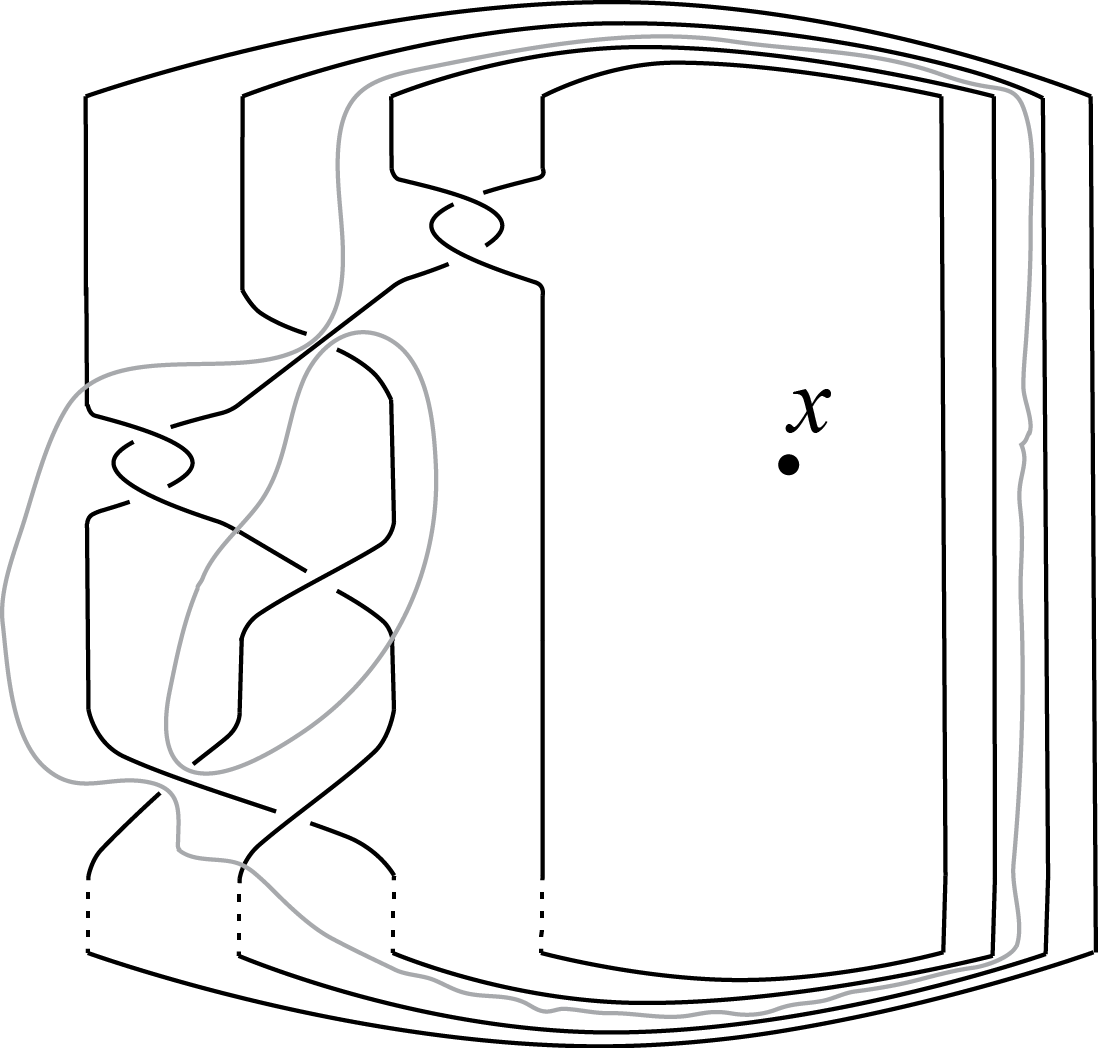
As before, let lie on the projection plane . A curve on will be called special with respect to if the following holds.
- (1)
intersects transversally in exactly four points. Denote them .
- (2)
intersects every edge of at most once.
- (3)
is monotone, i.e. it can be isotoped (where the intersection points of with the link may slide along a link strand until they reach a crossing, but not further) so that a ray from always intersects in a single point. Fig.5 (1) shows an example of a monotone curve, and Fig.5 (2) shows an example of a curve that is not monotone. If there is a choice whether put inside or outside of , while stays in the same region of , we always assume is outside of . This is illustrated in Fig.5 (3), where the curve is not monotone.
Note that the last condition above also implies that, up to isotopy, winds exactly once around .


Recall that by Lemma 2.1 (1), a Conway sphere in standard position results in either one or two curves in (similarly, in ). Modify a curve as follows. For every saddle it passes, push the curve from the saddle at a crossing into one of the edges adjacent to this crossing, as on Fig.1 (2). Call the new curve a modified curve. This modification does not correspond to an isotopy of .
Theorem 4.1.
Suppose is a reduced alternating diagram of a prime alternating non-split -braid . Assume contains a Conway sphere . Then either
- •
admits a special curve that is a or modified curve for or
- •
is a diagram of the -braid , where are positive integers.
Proof.
Note that for , we obtain an unknot that contains no essential surfaces. For , we obtain a -torus link, where an existence of a curve contradicts Lemma 2.1 (2), and a curve bounds a rational tangle. Hence, there are no Conway spheres, and the theorem holds vacuously. We therefore need to prove theorem for .
We claim that for , any or modified curve coming from either is special or bounds a 2-tangle whose diagram contains exactly one twist.
The curve cuts into two 2-tangles, and travels around not more than once, since it does not have self-intersections. In addition, cannot intersect an edge of more than once by Lemma 2.1 (2, 3).
If a curve enters a bigon through a saddle at a crossing (with ), it must exit the bigon through an edge (with ). But this contradicts Lemma 2.1 (2). Hence, if is a modified curve, it cannot intersect a bigon. If is an actual curve, it can be isotoped so that it does not cross any bigons.
Therefore, we can depict on the diagram from Fig.4 (1) so that if it passes through a black square, then the square represents a tangle with no crossings, and does not intersect in that square. The intersections of with can be grouped in consecutive pairs (a pair of intersections corresponds to entering/exiting a region of ), each pair arranged on a vertical, horizontal or diagonal line through a region of . There are four intersections of with , which can be denoted by . is a closed curve, and once a region where it starts is chosen, the fourth intersection, , must allow the curve to return to the same region.
Fig.6 shows all possible patterns once the starting region is chosen, and is placed on . In the figure, is depicted in gray, and dotted lines mean that more twisting may occur there. Between two consecutive points of intersection, and (up to cyclic order), the curve may pass through some black squares that have no crossings in them, without intersecting the link. To see that these are all possible patterns, note that must bound at least one twist, but is allowed only four intersections with . Call the twist : it is represented by a black square in the figure. Hence, a part of is necessarily a vertical segment between intersections with two strands of coming out of . Suppose the intersections are on the left of , and denote them by (for another side, the argument is similar). Then must close up in some way on the right from . Since there are just four intersections of with , and already has four strands, cannot go proceed to the left before and after . Fig.6 then demonstrates all ways for to close up, up to a symmetry/reflection, where the fact that other segments of must be horizontal, vertical or diagonal, is used.


Situation (1) includes either of the two possible ways of closing up : either making a full circle around , or through the shortest segment on the picture that connects its free ends. Fig.4 (2) shows an actual example of a braid and two curves that yield modified curves of types (1) and (3) from Fig.6.
In each of the depicted situations, either bounds just one twist of , or is monotone and therefore special. This concludes the proof of our claim.
Now consider the or curve represented by . Assume is not special. Then by the claim it bounds just one twist. If a curve bounds just one twist, is compressible. Hence, only a curve can bound a twist. The second curve coming from , denote it by , hits saddles at the same two crossings as . By the claim above, the modified curve resulting from either bounds a twist or is special itself.
If is special, we are done. Otherwise each of and bounds a twist. Then there are six twists in the diagram: two enclosed by and , two enclosed by the two modified curves in , and two one-crossing twists outside of all four of these modified curves. This is depicted in Fig.7, where are in grey color. Hence is a 3-braid. Each of the enclosed twists has just one crossing, since we isotoped so that a curve does not go through a crossing of a bigon of . Therefore, is the braid . ∎

5. Acknowledgements
We thank referee for the very careful reading of the paper. J. Hass acknowledges support from NSF grant DMS-1758107. A. Thompson acknowledges support from NSF grant DMS-1664587. A. Tsvietkova acknowledges support from NSF DMS-1664425 (previously 1406588) and NSF DMS-2005496 grants, and by Insitute of Advanced Study (under DMS-1926686 grant). All authors acknowledge support by Okinawa Institute of Science and Technology (OIST), Japan.
References
- [1] F. Bonahon and L. Siebenmann, New Geometric Splittings of Classical Knots, and the Classification and Symmetries of Arborescent Knots, Draft of a monograph.
- [2] J. Hass, A. Thompson, A. Tsvietkova, The number of surfaces of fixed genus in an alternating link diagram, Int. Math. Res. Not. (2017), no. 6, 1611–1622.
- [3] R. C. Kirby, W. B. R. Lickorish, Prime knots and concordance, Math. Proc. Cambridge Philos. Soc. 86 (1979), 437–441.
- [4] M. Lackenby, Classification of alternating knots with tunnel number one, Comm. Anal. Geom. 13 (2005), no. 1, 151–185.
- [5] W. B. R. Lickorish, Prime knots and tangles, Trans. Amer. Math. Soc. 267 (1981), no. 1, 321–332.
- [6] W. W. Menasco, Closed incompressible surfaces in alternating knot and link complements, Topology 23 (1984), 37–44.
- [7] W. Menasco, Determining incompressibility of surfaces in alternating knot and link complements, Pacific J. Math. 117 (1985), no. 2, 353–370.
- [8] W.W. Menasco, M. B. Thistlethwaite, The Tait flyping conjecture, Bull. Amer. Math. Soc. (N.S.) 25 (1991), no. 2, 403–412.
- [9] W.W. Menasco, M. B. Thistlethwaite, The Classififcation of Alternating Links, Ann. of Math. (2) 138 (1993), no. 1, 113–171.
- [10] M. B. Thistlethwaite, On the algebraic part of an alternating link, Pacific J. Math. 151 (1991), no. 2, 317–333.
Joel Hass
Department of Mathematics
University of California, Davis
One Shields Ave, Davis, CA 95616
hass@math.ucdavis.edu
Abigail Thompson
Department of Mathematics
University of California, Davis
One Shields Ave, Davis, CA 95616
thompson@math.ucdavis.edu
Anastasiia Tsvietkova
The Department of Mathematics and Computer Science
Rutgers University, Newark
101 Warren Street, Newark, NJ 07102
a.tsviet@rutgers.edu