Properties of Convex Optimal Power Flow Model Based on Power Loss Relaxation Journal: Electrical Power Systems Research
Abstract
We derive the branch ampacity constraint associated to power losses for the convex optimal power flow (OPF) model based on the branch flow formulation. The branch ampacity constraint derivation is motivated by the physical interpretation of the transmission line -model and practical engineering considerations. We rigorously prove and derive: (i) the loop constraint of voltage phase angle, required to make the branch flow model valid for meshed power networks, is a relaxation of the original nonconvex alternating current optimal power flow (o-ACOPF) model; (ii) the necessary conditions to recover a feasible solution of the o-ACOPF model from the optimal solution of the convex second-order cone ACOPF (SOC-ACOPF) model; (iii) the expression of the global optimal solution of the o-ACOPF model providing that the relaxation of the SOC-ACOPF model is tight; (iv) the (parametric) optimal value function of the o-ACOPF or SOC-ACOPF model is monotonic with regarding to the power loads if the objective function is monotonic with regarding to the nodal power generations; (v) tight solutions of the SOC-ACOPF model always exist when the power loads are sufficiently large. Numerical experiments using benchmark power networks to validate our findings and to compare with other convex OPF models, are given and discussed.
Keywords:
Optimal Power flow, ampacity constraint, tight solution, second-order cone programming.Nomenclature
Sets:
Nodes (or buses).
Lines (or branches).
Cycles (or closed loops).
Parameters:
Node to branch incidence matrices.
Longitudinal reactance and resistance
of branch modelled as a -model.
Shunt conductance and susceptance
of node .
Sending- and receiving- end shunt
susceptance of branch .
Actual and approximated ampacity
of branch .
Lower and upper bounds of .
Lower and upper bounds of .
Lower and upper bound of .
Active and reactive power loads
of node .
Cost parameters of active power
generation.
Variables:
Active and reactive power injections
at node .
Non-measurable sending-end active
and reactive power flows of branch .
Measurable sending-end active
and reactive power flows of branch .
Non-measurable receiving-end active
and reactive power flows of branch .
Measurable receiving-end active and
reactive power flows of branch .
Sending- and receiving- end shunt
reactive power of branch .
Non-measurable sending- and
receiving- end current of branch .
Measurable sending- and receiving-
end current of branch .
Active and reactive power losses of
branch .
Phase-to-ground voltage magnitude
and voltage square at node .
Sending- and receiving- end phase-to
-ground voltage of branch .
Sending- and receiving- end phase-to
-ground voltage square of branch .
Phase-to-ground voltage phase angle
at node .
Phase angle difference between
the sending- and receiving- end
phase-to-ground voltages of branch .
Phase angles of sending- and
receiving- end phase-to-ground
voltages of branch .
Equivalent ampacity constraint for
power losses of branch .
Indicators:
Relaxation gaps of active
power loss and reactive
power loss.
Maximum relaxation gaps
of .
1 Introduction
Optimal power flow (OPF) is a fundamental mathematical optimization model for decision making in power system operation and planning carpentier1962contribution. Improving the solution quality of OPF can give large economic and engineering benefits to the power industry Cain2012, advan_opt_meth_ps. Recent literature focusing on the convexification of the OPF model suffered from the inexactness due to the relaxation of several constraints Farivar2012_full, Gan2015, Kocuk2015, Bai2008, Lavaei2012, moment_relax_opf, sparcity_moment, qc_relax_minlp, Coffrin2015, stren_qc_bdt_pno, ttn_mcrelax_to_glob.
The branch flow formulation of the power flow equations for radial power networks has been originally derived by Baran and Wu in Capa_place_barawu to optimize the placement of capacitor in radial distribution networks. In Jabr2006, Jabr derives a conic programming approach to solve load flow in radial distribution network. In Farivar2012_full, Farivar and Low propose the branch flow model as a relaxed OPF model by relying on second-order cone programming (SOCP) and prove that the relaxation is tight for radial networks under the assumption that the upper bound of power generation is infinite. In Gan2015, Gan, Li et al. prove that the optimal solution of the branch flow model is exact (tight) if the voltage upper bounds are not binding and the network parameters satisfy some mild conditions which can be checked a priori. Christakou, Tomozei et al. show in Christakou2015 that the branch flow model is not exact due to the approximation of the branch ampacity constraint. Nick et al. propose an exact convex OPF model for radial distribution networks in Exact_OPF_rad by considering the shunt parameters associated to the exact modelling of the lines or other branch elements. Sufficient conditions regarding the network parameters under which the convex OPF model in Exact_OPF_rad can give exact solutions to the original ACOPF are provided and rigorously proved. In Kocuk2015, Kocuk, Dey et al. propose three methods (arctangent envelopes, dynamic linear inequalities and separation over cycle constraints) to strengthen or tighten the SOCP relaxation of OPF. Numerical results show better solution quality of SOCP-based model over SDP-based model Kocuk2015.
Semidefinite programming (SDP) relaxation of OPF has been firstly proposed by Bai et al. in Bai2008. The proposed procedures derive the rectangular form OPF in a quadratic programming model and replace the variable-vector (x) by the variable-matrix (). Solutions of OPF can be recovered from the square roots of the diagonal elements in the variable-matrix Bai2008. SDP advantages in avoiding the derivation of Jacobian and Hessian matrices if the interior point method (IPM) is used Bai2008. Lavaei and Low propose to solve the SDP relaxation of the dual OPF problem Lavaei2012. They prove that sufficient and necessary condition of zero duality gap holds for several IEEE test cases (14, 30, 57, 118) at the base power load level.11 1 As a comparison, in this paper, we evaluate the OPF solutions of test cases at low power load levels (for which the relaxation gaps are prominent). But the branch ampacity constraint is not fully addressed. Especially, as it is proved in Christakou2015, Exact_OPF_rad, the physical interpretation of the transmission line model is not correct in Lavaei2012. In Convex_Rel_mesh, Madani, Sojoudi et al. show that SDP relaxation works well if the line capacity is expressed by nodal voltage variables. A penalization method is proposed in Convex_Rel_mesh to reduce the rank of the SDP solution. Recenly, Eltved, Dahl et al. numerically investigate the computational efficiency of SDP by using test cases up to 82,000 nodes which is solved in around 7 hours using a high performance computing node SDP_rob_sca.
Based on polynomial optimization theory, Molzahn and Hiskens propose the moment-based relaxations of OPF in moment_relax_opf. This formulation firstly defines order- moment relaxation of all monomials of voltage real-and-imaginary components . Then, all the monomials up to order constitute the symmetric moment matrix which is used to re-formulate the OPF constraints via the SDP. Global optimal solutions are found, at the cost of heavy computational burden due to higher relaxation order , for the test cases in moment_relax_opf. The same authors in sparcity_moment improve the computational efficiency of this method by exploiting power system sparsity and applying high relaxation order to specific buses. In qc_relax_minlp, Hijazi, Coffrin et al. propose a quadratic convex (QC) relaxation by replacing the nonconvex voltage-amplitude-and-phase-angle associated constraints with the corresponding convex envelopes. In Coffrin2015, the same authors investigate the relationships between different convex OPF formulations including QC, SDP and SOCP. Reducing the optimality gap of QC or SOCP based OPF models by bound tightening techniques can be found in stren_qc_bdt_pno, ttn_mcrelax_to_glob. Recently, Shchetinin et al. propose in eff_bound_tight_relax three methods which require solving optimization problems to tighten the upper bounds of the voltage phase angle difference in order to satisfy the branch ampacity constraint. The same authors in construction_linear_app propose an iterative algorithm to construct a number of linear constraints (based on inner or outer approximation) to approximate the branch ampacity constraint.
In this paper, we focus on the formal derivation of equivalent ampacity constraint for the branch power losses. More specifically, we consider to improve the convex OPF model in radial and meshed power networks which necessitates the additional voltage phase angle constraint. Instead of using the approach in Exact_OPF_rad to reformulate the branch flow model, we keep using the same set of variables (in the form of power flow variables) of the branch flow model but equivalently derive the ampacity constraint for the power losses. In this way, we overcome the approximation gap due to neglecting of the shunt elements of the branches. We then propose and prove six theorems showing important properties of the proposed SOC-ACOPF model. In this regard, the main contributions of this paper are listed below.
- •
Derivation of the transmission line or branch ampacity constraint for the power losses.
- •
Proving that the SOC-ACOPF model (with additional constraint to improve its feasibility) is a relaxed ACOPF model.
- •
Deriving a feasible solution recovery procedure when the SOC relaxation is tight.
- •
Demonstrating that the (parametric) optimal value functions of the SOC-ACOPF model and o-ACOPF model are monotonic with regarding to the power loads when the objective function is monotonic with regarding to the power generations.
- •
Proving that larger power loads can tighten the relaxation in the SOC-ACOPF model.
- •
Numerical Comparison of our o-ACOPF model and SOC-ACOPF model with respect to the other two convex OPF models proposed in the recent literature.
The rest of this paper is organized as follows. Section II formulates the o-ACOPF model and SOC-ACOPF model for radial and meshed power networks. Section III derives the equivalent branch ampacity constraint for power losses. Section IV proposes and proves important properties of the SOC-ACOPF model. Section V gives the numerical validations of our analytical proofs and discussions. A numerical comparison with other convex OPF models is also conducted. Section VI concludes.
2 Optimal Power Flow Model
2.1 Power based Branch Flow Model
We assume that the three-phase power grid satisfies two conditions: (i) all the branches and shunt impedances are circularly symmetric; (ii) all the triplets of nodal voltages and branch currents are symmetrical and balanced. These two conditions validate the use of single-line equivalent model of the three-phase power grid. The full ACOPF model is based on the validated branch flow model presented in DLMP_me. We denote this original ACOPF model as o-ACOPF model-(1). The variable convention makes reference to the branch -model in Fig. 1. are the longitudinal reactance and resistance of branch . are the sending- and receiving- end shunt susceptance of branch . is the phase-to-ground voltage magnitude at node . are the non-measurable sending-end active and reactive power flows of branch . are the measurable sending-end active and reactive power flows of branch . are the non-measurable receiving-end active and reactive power flows of branch . are the measurable receiving-end active and reactive power flows of branch . are the sending- and receiving- end shunt reactive power of branch . The subscripts in are not indices but to imply the meaning of sending-end of branch , receiving-end of branch , power load, power loss and shunt capacitance correspondingly.

Note are the actual (i.e. measurable) branch power flows. The variables are the non-measurable branch power flows used in our OPF model. For the difference between and , or between and , please refer to references Christakou2015 and Exact_OPF_rad. We want to emphasize here that the physical interpretation of the branch -model is of importance since the branch phase-to-ground capacitance is actually distributed along the branch which means the current (or power) flowing through the branch is actually not the same along the branch due to the charging current (or power) flowing from the distributed phase-to-ground capacitance to the branch. Although the distributed branch phase-to-ground capacitance is represented in the -model in a lumped way at the two-ends of the branch, we should bear in mind that the current, or the power, along the branch is not the same when we consider the branch ampacity constraint. This means that the actual power flow variables are non-measurable and difficult to be constrained. This is the main reason we only rely on the measurable power flow variables to constrain the branch ampacity and then derive the relationship between and later in this paper.
| (1a) | ||||
| subject to | ||||
| (1b) | ||||
| (1c) | ||||
| (1d) | ||||
| (1e) | ||||
| (1f) | ||||
| (1g) | ||||
| (1h) | ||||
| (1i) | ||||
| (1j) | ||||
| (1k) | ||||
| (1l) | ||||
| (1m) | ||||
| (1n) | ||||
| (1o) | ||||
Where is the set of model variables. is the dimension of . is the cardinality of the node set . is the cardinality of the branch set . is the index of nodes. is the index of branches. Based on the applications, the objective function can be the economic cost of energy production or network power losses etc. In this paper, we assume the objective function is convex. Equations (1b) and (1c) represent the active and reactive power balance. are the shunt conductance and susceptance of node . and are the node-to-branch incidence matrices of the network with if is the sending-end of branch , and if is the receiving-end of branch . are the active and reactive power generations at node . are the active and reactive power loads at node . is the phase-to-ground voltage magnitude square at node . are the active and reactive power losses of branch . Constraints (1b)-(1e) make the o-ACOPF model valid for both radial and meshed power networks. Equations (1d)-(1e) are derived by taking the magnitude and phase angle of the voltage drop phasor along branch respectively. are the sending- and receiving- end phase-to-ground voltages of branch . are voltage magnitude squares. is the phase angle difference between the sending- and receiving- end voltages of branch . are the phase angles of sending- and receiving- end phase-to-ground voltages of branch . To guarantee this derivation is valid, we assume . are the non-measurable sending- and receiving- end currents of branch . are the measurable sending- and receiving- end currents of branch . is the actual ampacity of branch which is provided by the branch manufacturer. Equations (1i)-(1j) represent active power and reactive power losses. Constraints (1k)-(1o) are bounds for voltage magnitude, voltage phase angle difference, nodal active power generation and nodal reactive power generation. are the lower and upper bounds of . are the lower and upper bounds of . are the lower and upper bounds of . This model is nonconvex because of the nonconvex constraints (1e), (1g), (1i) and (1j). It is hard for current available nonlinear programming solvers to efficiently find the global optimal solution of this nonconvex optimization model.
It is worth to mention that including as one of the model variables and using (1h) to define make our model implicitly satisfy the cyclic constraint (Kirchoff’s voltage law for AC circuit) of meshed power networks:
| (1p) |
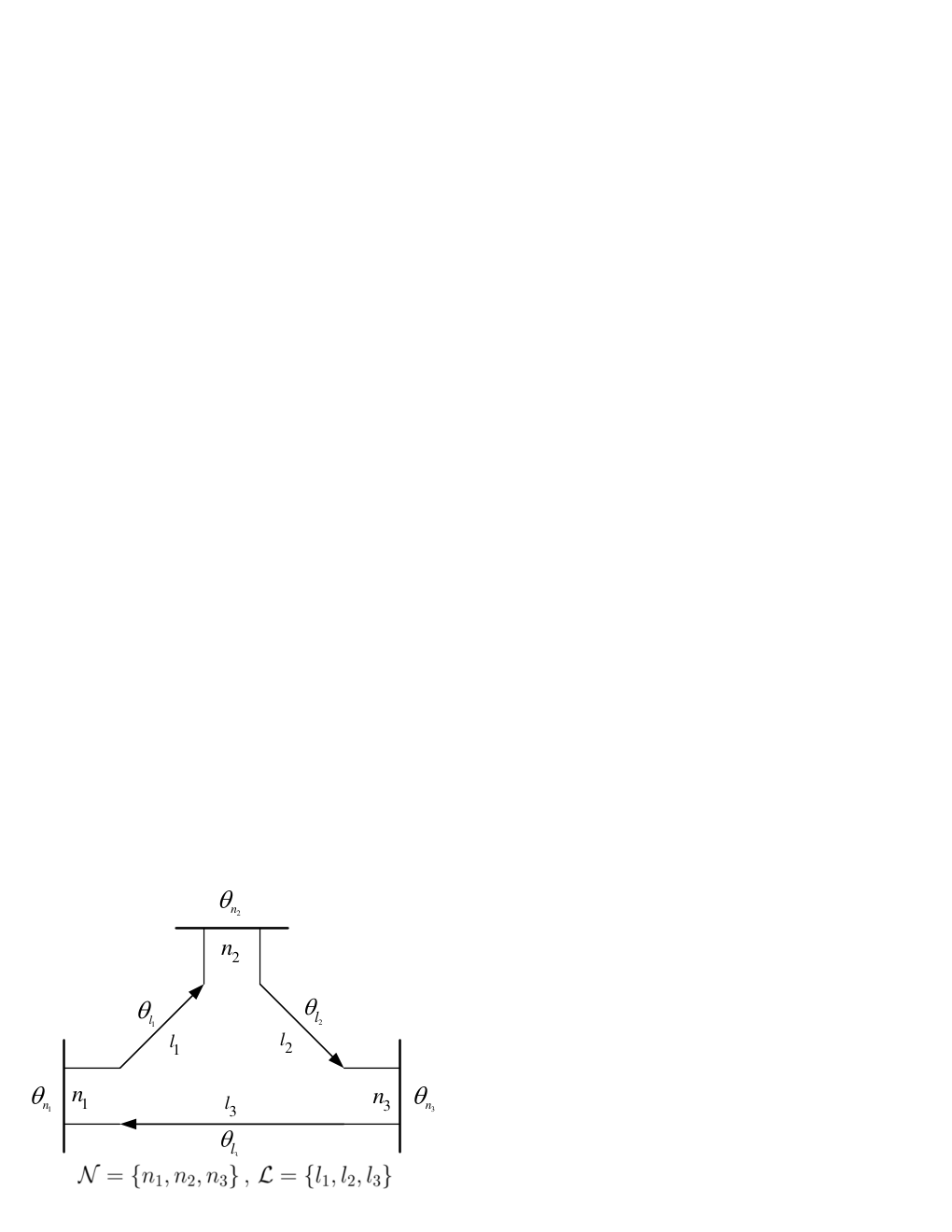
Where is the set of all cycles or closed loops in the meshed power networks. This means we do not need to include the cyclic constraint (1p) explicitly in our model. This approach is used and validated by our work in DLMP_me, SOCACOPF_relax_fea_me. An illustrative example is provided in Fig. 2. In this example, since , and , the cyclic constraint is implicitly satisfied. This reasoning holds for cycles or closed loops with any number of nodes and branches.
2.2 Second-Order Cone Relaxation
The SOC-ACOPF model is derived using branch sending-end power flows and voltage phase angle variables. Note that in the derived model, voltage magnitude square variables are used (voltage magnitude can be recovered from the model by taking the square root of the solutions of the voltage magnitude square variables). Our SOC-ACOPF is formulated in optimization model-(2). The numerical performance of this model compared with other SOCP based ACOPF models can be found at SOCACOPF_relax_fea_me.
| (2a) | ||||
| (2b) | ||||
| (2c) | ||||
| (2d) | ||||
Where is the set of model variables. Since we only use voltage magnitude square variable in this SOC-ACOPF model, the voltage magnitude constraint (1k) is modified as in the SOC-ACOPF model-(2). Constraints (2b)-(2c) represent active power and reactive power losses. are the equivalent ampacity constraint for power losses of branch . These constraints are relaxed from constraints (1i)-(1j) in the o-ACOPF model-(1). The left side of constraint (2b) bounds , which equivalently bounds the ampacity of branch as explained in the next section. Note even though the right side of constraint (2b) is not in the standard form of SOCP, it can be equivalently transformed to a rotated SOCP constraint as . We keep the original format of the right side of constraint (2b) in the SOC-ACOPF model-(2) because the physical meaning is more clear. Equation (2d) is derived from the nonconvex constraint (1e). This derivation is based on the assumption . The left side of equation (2d) can also be derived by the first-order Taylor series expansion of at and . We will show later that using (2d) actually relaxes the ACOPF model when and . It is worth to mention that even though constraint (2d) is the only constraint associated with the voltage phase angle variable, it should be solved jointly with other constraints in order to guarantee the feasibility of .
3 Deriving the Branch Ampacity constraint for the Power Losses
Since the actual measurable power flows and current are different from the power flow variables and that we are using in the SOC-ACOPF model-(2), it is necessary to derive the gap between and to derive according to the known parameter . From Fig. 1, we have:
| (3a) | ||||
| (3b) | ||||
| (3c) | ||||
| Where is the reactive power injection from the sending- (receiving-) end shunt capacitance of the branch , is the shunt susceptance. The branch ampacity constraint is: | ||||
| (3d) | ||||
| From (3a)-(3d), we can derive the gap between and as: | ||||
| (3e) | ||||
| The branch ampacity constraint (3d) is equivalent to: | ||||
| (3f) | ||||
| The reactive power losses upper bounds can be quantified as: | ||||
| (3g) | ||||
Note equation (3g) is linear. So, if we use the expression of from (3g) in the constraint (2b), the SOC-ACOPF model-(2) is still convex and we avoid any approximation on the branch ampacity constraint.
It is worth to mention that using to limit the upper bound of power losses in (2b) is more realistic than constraining the power flows or in the way of or (where is the maximum branch power flow). This is because:
- •
(i) the branch ampacity is given by the manufacturers in the form of maximum current .
- •
(ii) the temperature increase of the branch (which lead to insulation degrading) is actually caused by the power losses due to the current which is the typical variable constrained by the branch manufacturer.
- •
(iii) the voltage amplitudes of both ends of the branch are varying during the power network operations. The maximum allowed power capacity of the branch would then depend on the nodal voltage amplitudes at the branch ends.
4 Properties of the SOC-ACOPF Model
In order to rigorously prove the important properties of the SOC-ACOPF mdoel-(2) and the o-ACOPF model-(1), we firstly give the definitions of some key words. Some well-defined terms in the control and optimization community are also re-stated here for sake of readability. For ease of illustration, all the mentioned optimization models in this paper are assumed as minimization problems i.e. we consider minimizing the objective functions. Maximization problems can be equivalently transformed to minimization problems by minimizing the negative of the objective functions (of the maximization problems). If multiple optimization models are mentioned in one definition or theorem here, unless otherwise specified, we always mean that they have the same objective function. Note here we use the symbols and to denote two general optimization models. Our ACOPF model-(1) and SOC-ACOPF model-(2) can be regarded as examples of the optimization models and .
| Theorem | Property |
|---|---|
| 1 | The SOC-ACOPF model-(2) is a relaxation of the o-ACOPF model-(1). |
| 2 | Necessary condition to recover feasible solution of the o-ACOPF model-(1) from the solution of the SOC-ACOPF model-(1). |
| 3 | The SOC-ACOPF model-(2) with the additional constraint (4g) is still a relaxation of the o-ACOPF model-(1). |
| 4 | Recover the global optimal solution of the o-ACOPF model-(1) from the solution of the SOC-ACOPF model-(2). |
| 5 | The parametric optimal value functions of the o-ACOPF model-(1) and the SOC-ACOPF model-(2) are monotonic. |
| 6 | Tight solution of the SOC-ACOPF model-(2) always exist. |
Definition \@upn1
Feasible solution. A feasible solution of an optimization model is the solution satisfying jointly all the constraints of .
Definition \@upn2
Feasible region. The feasible region of an optimization model is the set of all feasible solutions of .
Definition \@upn3
Global optimal solution. A global optimal solution of an optimization model is the feasible solution of which gives the minimal (for minimization problem) objective function value i.e. .
Definition \@upn4
Definition \@upn5
Relaxation. An optimization model is said to be a relaxation or a relaxed model of optimization model if and only if the feasible region of is a subset of the feasible region of i.e. .
Definition \@upn6
Approximation. An optimization model is said to be an (strict) approximation or an approximated model of optimization model if and only if the feasible regions of and are approximately equal but neither one is a subset of another i.e. .
Definition \@upn7
Relaxation gap. For the SOC-ACOPF model-(2), the relaxation gap of active power loss is defined as:
| (4a) |
The relaxation gap of reactive power loss is defined as:
| (4c) |
To give an overview of the proposed theorems, we summarize the theorems in Table 1. Theorem 4 is a based on theorem 1, theorem 2 and thorem 3. Theorem 6 is based on theorem 5.
Theorem \@upn1
Proof.
We prove this theorem by showing that any point in the feasible region of o-ACOPF model-(1) can always be mapped to a point located in the feasible region of the SOC-ACOPF model-(2). However, the reverse statement does not hold. In other words, some feasible solutions of the SOC-ACOPF model-(2) are not feasible for the o-ACOPF model-(1). This means the feasible region of the SOC-ACOPF model-(2) covers the feasible region of the o-ACOPF mode-(1).
Theorem 1 shows that the feasible region of SOC-ACOPF model-(2) covers all the feasible region of o-ACOPF model-(1). It is worth to mention that the assumptions of and are the practical operational requirements for power system. These assumptions can be relaxed to some degree while Theorem 1 is still valid.
Theorem \@upn2
Proof.
Theorem 2 shows that if we add the convex constraint (4g) to the SOC-ACOPF model-(2), we can improve the solution feasibility towards the o-ACOPF model-(1). Please note that equations (4h)-(4j) is only one way to recover the feasible solution. Condition (4g) is necessary to recover the feasible solution by using this approach. There can be other feasible solution recovery approaches which do not require condition (4g).
Theorem \@upn3
Proof.
We can use the same procedure in proving theorem 1 to prove theorem 3 i.e. any feasible solution of the o-ACOPF model-(1) can be mapped to a feasible solution of the SOC-ACOPF model-(2) with the additional constraint (4g). However, the reverse statement is not true when there is at least one (in the feasible solution of the SOC-ACOPF model-(2) with the additional constraint (4g)) such that (which fails to satisfy constraints (1j) in the o-ACOPF model-(1) obviously). ∎
Theorem 3 shows that the SOC-ACOPF model-(2) with the additional constraint (4g) still covers the feasible region of the o-ACOPF model-(1).
Theorem \@upn4
Proof.
Theorem \@upn5
Define the (parametric) optimal value functions:
| (4m) | ||||
| (4n) |
Where and are the feasible regions of the o-ACOPF model-(1) and the SOC-ACOPF model-(2) correspondingly. If the objective function is a monotonically increasing function of i.e. for , the optimal value functions are monotonic i.e. for (assuming the o-ACOPF model-(1) and the SOC-ACOPF model-(2) are feasible for and ).
Proof.
We prove theorem 5 by contradiction. Suppose the optimal solutions and objectives of the SOC-ACOPF model-(2) (or the o-ACOPF model-(1)) at and are and . If for , since is monotonic, there must be at least one such that . We can construct a feasible solution of the SOC-ACOPF model-(2) (or the o-ACOPF model-(1)) at (by using ) as:
| (4o) |
| (4p) | ||||
| (4q) |
We know the feasible solution of must satisfy:
| (4r) | ||||
| (4s) |
Substituting (4r)-(4s) to (4p)-(4q), we have:
| (4t) | ||||
| (4u) |
Which yield:
| (4v) | ||||
| (4w) |
So is feasible for the SOC-ACOPF model-(2) (or the o-ACOPF model-(1)). Because , equations (4v)-(4w) imply . This means the corresponding objective function values satisfy (note ) which contradicts the assumption that is the optimal objective solution. So cannot hold for . This completes the proof. ∎
Theorem \@upn6
Proof.
To prove theorem 6, we firstly derive an equivalent model of the o-ACOPF model-(1) by replacing constraint (1d) with:
| (4x) |
Constraints (4x)-and-(1e) are equivalent with constraints (1d)-and-(1e) for since they are expressing the same voltage drop phasor either in the way of real-and-imaginary parts or amplitude-and-imaginary parts illustrated in Fig. 3.
We then define a new relaxed ACOPF model as r-ACOPF in (4y).
| (4y) | ||||
Obviously, when the relaxation is tight, the feasible region of the r-ACOPF model-(4y) is actually equivalent to the feasible region of the SOC-ACOPF model-(2) (with the additional constraint (4g)) since any feasible solution from either model (SOC-ACOPF model-(2) or r-ACOPF model-(4y)) can be mapped to the feasible region of another model (SOC-ACOPF model-(2) or r-ACOPF model-(4y)) using the procedures we derived in theorems 1-4. The feasible region comparison is shown in Fig. 4.
We want to emphasize here that, although the r-ACOPF model-(4y) is nonconvex (with regarding to its own set of variables), it is valid that part of its feasible region can be mapped to a convex one (with another set of variables) such as the convex SOC-ACOPF model-(2) (with additional constraint (4g)). An obvious simple example is the equivalence between the nonconvex region expressed by for and convex region expressed by for . Fig. 5 shows this equivalence graphically. A similar consideration can be drawn for the r-ACOPF model-(4y) (where both and are deployed) and the SOC-ACOPF model-(2) where only are used.
Similarly, we define the (parametric) optimal value function of the r-ACOPF model-(4y) (with regarding to ) as:
| (4z) |
Following the same procedure in the proof of theorem 5, it is obvious that here is also monotonic.
We now use the r-ACOPF model-(4y) as a bridge to prove theorem 6. The key procedure is to show that theorem 6 is valid for the r-ACOPF model-(4y) and thus valid for the SOC-ACOPF model-(2) considering the equivalence between their feasible regions (when the relaxation is tight). Suppose the optimal solution of the r-ACOPF model-(4y) has positive relaxation gap or for some at , we use and to represent the active and reactive power losses relaxation gaps respectively:
| (4aa) | ||||
| (4ab) |
So the tight power losses solutions are and . From constraints (1b)-(1c), we have:
| (4ac) |
| (4ad) |
Suppose at , tight power losses solutions are found (note in the r-ACOPF model-(4y) only the following constraints are associated with the power losses variables aside from constraints (2b)-(2c)):
| (4ae) | ||||
| (4af) |
Combining equations (4ac)-(4ad) with equations (4ae)-(4af), we have:
| (4ag) | ||||
| (4ah) |
Because and , equations (4ag)-(4ah) imply . Taking into account that the optimal value function is monotonic, we also know that which means is not only feasible but also optimal for the r-ACOPF model-(4y) at . As we have explained at the beginning of this proof, since the r-ACOPF model-(4y) is actually equivalent (in terms of the feasible region and optimal solution when the relaxation is tight) with the SOC-ACOPF model-(2), all the tight solutions we derived in proving theorem 6 for the r-ACOPF model-(4y) can always be mapped to the corresponding tight solution of the SOC-ACOPF model-(2). In other words, theorem 6 is also valid for the SOC-ACOPF model-(2). ∎
Theorem 6 shows the structure of the relaxed solutions and tight solutions for the SOC-ACOPF model-(2) with regarding to the power load parameter. This theorem shows a counter-intuitive property of the SOC-ACOPF model-(2) that larger power load can help tighten the relaxation gap. We present in the next Section the numerical validations of all the theorems and analysis in this Section.
| Test case | 10% Load | 20% Load | 30% Load | 40% Load | ||||
| SOC-ACOPF | o-ACOPF | SOC-ACOPF | o-ACOPF | SOC-ACOPF | o-ACOPF | SOC-ACOPF | o-ACOPF | |
| case4 | 2.40107 | 2.40107 | 4.80428 | 4.80428 | 7.20965 | 7.20965 | 9.6171 | 9.6171 |
| case9 | 1170.74 | 1170.75 | 1347.23 | 1347.23 | 1593.64 | 1593.64 | 1909.78 | 1909.78 |
| 13feeder | 0.00745 | 0.00745 | 0.01493 | 0.01493 | 0.02245 | 0.02245 | 0.03002 | 0.03002 |
| IEEE14 | 545.64 | 546.37 | 1147.21 | 1147.50 | 1806.10 | 1806.26 | 2523.77 | 2523.91 |
| case30 | 33.14 | 33.14 | 75.31 | 75.31 | 123.61 | 123.61 | 178.12 | 178.12 |
| 34feeder | 0.00211 | 0.00211 | 0.00426 | 0.00426 | 0.00645 | 0.00645 | 0.00868 | 0.00868 |
| IEEE57 | 2682.55 | 2686.41 | 5706.04 | 5709.00 | 9080.48 | 9082.93 | 12809.00 | 12810.65 |
| IEEE118 | 8940.49 | 8952.62 | 18735.71 | 18750.11 | 29420.72 | 29436.19 | 41008.27 | 41025.36 |
| ACTIVSg200 | 14070.44 | 14070.44 | 14070.44 | 14070.44 | 14070.44 | 14070.44 | 14483.45 | 14483.82 |
| IEEE300 | 51210.16 | 56915.23 | 107284.01 | 108378.18 | 168588.72 | 168712.09 | 235157.51 | 235244.97 |
| ACTIVSg500 | 16386.94 | 16386.94 | 16386.94 | 16386.94 | 16386.94 | 16386.94 | 16386.94 | 16386.94 |
| 1354pegase | 7558.35 | 7558.47 | 15101.85 | 15102.06 | 22665.28 | 22665.88 | 30246.88 | 30249.40 |
| ACTIVSg2000 | 301722.90 | 301722.90 | 319936.30 | 321123.46 | 401882.50 | 402289.24 | 509723.50 | 510082.88 |
| 2383wp | 0.00 | 0.00 | 0.00 | 0.00 | 19377.99 | 19477.73 | 175742.10 | 175881.88 |
| 2736sp | 0.00 | 0.00 | 0.00 | 0.00 | 108775.80 | 108838.81 | 250447.80 | 250617.91 |
| 2737sop | 0.00 | 0.00 | 5.86 | 5.86 | 42096.36 | 42110.97 | 128947.20 | 128979.20 |
| 2869pegase | 14639.05 | 14754.46 | 29204.10 | 29236.82 | 43811.78 | 43830.34 | 58458.84 | 58467.05 |
| 3012wp | 0.00 | 0.00 | 0.00 | 0.00 | 41101.36 | 41261.04 | 338807.19 | 339179.85 |
| 3120sp | 1336861.76 | 1336861.82 | 1336861.76 | 1336861.82 | 1336861.76 | 1336861.82 | 1336861.76 | 1336861.82 |
| 3375wp | 6418725.22 | 6418725.36 | 6418725.22 | 6418725.37 | 6418725.22 | 6418725.36 | 6418725.22 | 6418725.36 |
| Test case | 10% Load | 10% Load | 20% Load | 20% Load | 30% Load | 30% Load | 40% Load | 40% Load |
| case4 | 9.75E-11 | 8.46E-10 | 1.00E-10 | 8.27E-10 | 1.00E-10 | 6.82E-10 | 9.85E-11 | 8.51E-10 |
| case9 | 9.82E-11 | 1.59E-16 | 5.65E-11 | 3.60E-13 | 1.16E-10 | 2.95E-13 | 9.81E-11 | 3.02E-12 |
| 13feeder | 1.24E-7 | 6.42E-9 | 1.24E-7 | 6.43E-9 | 1.23E-7 | 6.38E-9 | 1.22E-7 | 6.19E-9 |
| IEEE14 | 5.43E-10 | 7.31E-13 | 3.35E-09 | 6.89E-13 | 1.06E-10 | 6.85E-12 | 2.99E-09 | 1.45E-12 |
| case30 | 5.45E-10 | 6.47E-10 | 1.67E-10 | 1.33E-11 | 1.71E-09 | 1.72E-10 | 1.21E-10 | 1.84E-10 |
| 34feeder | 1.25E-7 | 6.98E-9 | 1.25E-7 | 6.82E-9 | 1.25E-7 | 6.68E-9 | 1.25E-7 | 2.40E-9 |
| IEEE57 | 1.84E-10 | 5.92E-10 | 2.52E-11 | 7.46E-10 | 1.36E-09 | 2.09E-10 | 6.38E-09 | 8.26E-10 |
| IEEE118 | 4.93E-09 | 3.28E-09 | 6.02E-08 | 1.79E-09 | 1.11E-07 | 1.10E-09 | 1.57E-09 | 3.99E-11 |
| ACTIVSg200 | 1.67E-02 | 1.28E-10 | 1.43E-02 | 3.37E-10 | 6.65E-03 | 6.97E-10 | 1.45E-08 | 5.79E-10 |
| IEEE300 | 1.15E-02 | 4.14E-08 | 1.37E-03 | 8.17E-09 | 4.08E-06 | 2.52E-09 | 5.01E-05 | 1.10E-09 |
| ACTIVSg500 | 2.29E-02 | 1.34E-09 | 2.12E-02 | 3.69E-09 | 1.93E-02 | 5.49E-10 | 1.60E-02 | 3.59E-10 |
| 1354pegase | 3.09E-03 | 1.79E-07 | 2.72E-07 | 1.42E-07 | 1.01E-02 | 1.43E-07 | 1.04E-02 | 1.03E-07 |
| ACTIVSg2000 | 2.14E-01 | 5.55E-08 | 1.09E-01 | 9.87E-09 | 5.26E-02 | 1.93E-08 | 4.10E-02 | 1.03E-08 |
| 2383wp | 1.94E-01 | 3.65E-08 | 1.77E-01 | 3.11E-08 | 2.52E-03 | 1.28E-08 | 7.46E-03 | 4.29E-08 |
| 2736sp | 2.10E-02 | 9.68E-09 | 3.22E-10 | 2.57E-08 | 2.85E-08 | 9.64E-09 | 3.58E-04 | 5.74E-10 |
| 2737sop | 3.32E-02 | 5.12E-08 | 1.45E-02 | 3.75E-08 | 4.56E-08 | 2.89E-08 | 1.65E-03 | 2.35E-08 |
| 2869pegase | 8.47E-03 | 7.12E-06 | 9.32E-03 | 1.38E-07 | 6.72E-03 | 6.56E-08 | 1.47E-02 | 6.99E-08 |
| 3012wp | 1.09E-01 | 4.21E-06 | 2.35E-02 | 4.64E-09 | 1.69E-03 | 3.78E-11 | 4.75E-04 | 3.08E-11 |
| 3120sp | 1.01E+01 | 2.85E-09 | 7.48E+00 | 1.72E-11 | 3.56E+00 | 2.72E-11 | 1.28E+00 | 5.18E-11 |
| 3375wp | 7.22E+00 | 5.06E-10 | 5.40E+00 | 6.82E-8 | 3.12E+00 | 2.43E-10 | 1.39E+00 | 1.05E-8 |
| Test case | 10% Load | 10% Load | 20% Load | 20% Load | 30% Load | 30% Load | 40% Load | 40% Load |
| case4 | 1.95e-10 | 1.69e-9 | 2.01e-10 | 1.65e-9 | 2.01e-10 | 1.36e-9 | 1.97e-10 | 1.70e-9 |
| case9 | 3.65E-01 | 1.16E-10 | 1.57E-01 | 3.06E-12 | 1.33E-01 | 4.70E-12 | 1.14E-01 | 1.63E-11 |
| 13feeder | 3.42E-7 | 2.42E-9 | 3.40E-7 | 2.40e-9 | 3.37E-7 | 2.37E-9 | 3.35E-7 | 2.34E-9 |
| IEEE14 | 2.50E-01 | 8.51E-11 | 7.95E-02 | 3.92E-11 | 1.43E-01 | 1.24E-10 | 1.18E-01 | 2.33E-11 |
| case30 | 2.31E-02 | 1.78E-09 | 2.34E-02 | 2.65E-11 | 2.21E-02 | 3.66E-10 | 2.04E-02 | 3.79E-10 |
| 34feeder | 3.10E-7 | 2.43E-9 | 3.03E-7 | 2.43E-9 | 2.97E-7 | 2.44E-9 | 2.90E-7 | 8.94E-10 |
| IEEE57 | 2.25E-01 | 2.00E-09 | 1.92E-01 | 9.65E-09 | 1.46E-01 | 3.10E-09 | 1.02E-01 | 3.37E-09 |
| IEEE118 | 2.98E+00 | 1.00E-08 | 3.08E+00 | 1.37E-08 | 2.86E+00 | 9.55E-09 | 2.84E+00 | 3.03E-09 |
| ACTIVSg200 | 2.05E-01 | 1.35E-09 | 1.99E-01 | 1.94E-09 | 2.09E-01 | 7.14E-09 | 1.06E-06 | 2.91E-09 |
| IEEE300 | 5.25E+00 | 9.33E-08 | 4.12E+00 | 1.75E-08 | 3.82E+00 | 3.26E-08 | 3.62E+00 | 6.55E-08 |
| ACTIVSg500 | 3.31E-01 | 1.41E-08 | 2.87E-01 | 4.88E-08 | 2.45E-01 | 7.27E-09 | 2.33E-01 | 4.74E-09 |
| 1354pegase | 2.95E-01 | 1.46E-06 | 2.93E-01 | 3.45E-07 | 8.50E-01 | 4.77E-07 | 8.74E-01 | 2.63E-07 |
| ACTIVSg2000 | 2.23E+00 | 2.10E-07 | 2.57E+00 | 8.57E-08 | 2.56E+00 | 1.36E-07 | 2.53E+00 | 4.70E-08 |
| 2383wp | 1.87E+00 | 2.85E-07 | 1.61E+00 | 2.34E-07 | 1.13E-01 | 4.60E-08 | 3.34E-01 | 8.70E-08 |
| 2736sp | 2.37E-01 | 4.94E-08 | 1.19E-03 | 1.21E-07 | 1.18E-03 | 3.93E-08 | 1.48E-02 | 1.74E-09 |
| 2737sop | 3.76E-01 | 1.82E-07 | 1.58E-07 | 3.13E-07 | 1.19E-03 | 1.76E-07 | 1.17E-01 | 1.39E-06 |
| 2869pegase | 7.81E-01 | 4.96E-05 | 5.03E-01 | 3.44E-06 | 3.79E-01 | 8.79E-07 | 2.64E+00 | 1.12E-06 |
| 3012wp | 6.23E-01 | 1.01E-10 | 3.36E-01 | 1.00E-10 | 1.54E+00 | 1.16E-10 | 1.33E+00 | 9.91E-11 |
| 3120sp | 3.10E+01 | 1.01E-10 | 1.29E+01 | 9.92E-11 | 6.13E+00 | 9.90E-11 | 1.58E+00 | 9.88e-11 |
| 3375wp | 7.52E+00 | 4.72E-10 | 4.67E+01 | 4.67E-10 | 3.12E+01 | 4.56E-10 | 2.75E+01 | 4.45E-10 |
5 Numerical results and discussion
The SOC-ACOPF model-(2) (with the additional constraint (4g)) and o-ACOPF model-(1) are implemented and solved in the YALMIP yalmip_toolbox toolbox for modelling and optimization in MATLAB and Julia julia_fresh running on the 64-bit macOS operating system. A personal computer with Intel Core i9 2.9 GHz CPU and 16G RAM is deployed. The MOSEK, Gurobi, SCS solvers are used to solve the SOC-ACOPF model-(2). Because MOSEK, Gurobi and SCS can only solve convex models, the convexity of the SOC-ACOPF model-(2) is numerically validated. The IPOPT solver is used to solve the nonconvex o-ACOPF model-(1).
5.1 Validation of Theorems 1-6
We use benchmark IEEE transmission networks {14, 57, 118, 300}, matpower case 9, 30, ACTIVSg {200, 500, 2000}, 2383wp, 2736sp, 2737sop, 3012wp, 3120sp, 3375wp, {1354, 2869} pegase Fliscounakis and the distribution networks case4, 13feeder, 34feeder as the test cases to numerically validate the proposed theorems for both power transmission and distribution networks in this Section. Power network data from MATPOWER are directly used here Zimmerman2011. Note the 3012wp, 3120sp and 3375wp networks are stressed test cases for the winter peak (wp) time or summer peak (sp) time. The objective function of typical economic dispatch is quadratic i.e. . Where are the cost parameters of nodal active power generation. Note some cost parameters of the generators are equal to zero in the test cases. So in some low power load scenarios, the total generation cost is equal to zero or remains the same with the increase of power loads. For the distribution networks, we include several distributed generators with positive cost parameters in all the networks. To make sure the objective function is monotonic for , we must ensure in the o-ACOPF and SOC-ACOPF models. For large test cases with over 3000 nodes, we use Julia to implement and solve both the SOC-ACOPF model-(2) and the o-ACOPF model-(1). This is mainly due to the higher computational efficiency of Julia compared with YALMIP with the associated optimization solvers.
Since we have tested our models for the base power loads (original power loads in MATPOWER) and shown in our previous work SOCACOPF_relax_fea_me that large relaxation gaps are present for optimal solutions in low power loads scenarios, we only show the results for low power loads scenarios here. In Table 2, we list the objective solutions of the SOC-ACOPF model-(2) and the o-ACOPF model-(1) for 10%, 20%, 30% and 40% of the absolute value of base load. So, the results in Table 2 validate theorems 1-5:
- •
- •
The (parametric) optimal value functions of the SOC-ACOPF model-(2) and the o-ACOPF model-(1) are monotonic (with regarding to the power load ) given that the objective function is monotonic with regarding to the power generation . This is validated since all the objective solutions increase when the power loads increase.
For the SOC-ACOPF model-(2). The maximum relaxation gaps of active and reactive power losses are defined as:
| (5a) | ||||
| (5b) | ||||
We use and to measure the relaxation performance of the SOC-ACOPF model-(2) (smaller relaxation gaps mean better performance). We list the maximum relaxation gaps results and of the SOC-ACOPF model-(2) in Table 3 and Table 4. When the relaxation is not tight, we increase the power load levels (but fix the optimal nodal power generation solution so the objective solutions remain the same as in Table 2) to find the tight solutions of the SOC-ACOPF model-(2). The power load levels are increased by taking the power loads as variables in the SOC-ACOPF model and using the original power load levels (10%, 20%, 30% and 40%) as the lower bounds of these variables. The maximum relaxation gaps for tight solutions are listed in the columns denoted as ’10% Load’, ’ 20% Load’, ’ 30% Load’ and ’ 40% Load’ of Table 3 and Table 4. So we have actually numerically validated theorem 6 by the results in Table 3 and Table 4. It is worth to mention that for most branches, the relaxation gaps are very small. The maximum relaxation gap only appear for single branch in each test case i.e. there is only one branch in each test case such that or .
| Test case | SOC-ACOPF | o-ACOPF | OPF Model in qc_relax_minlp | OPF Model in Jabr2006 |
| case4 | 24.11 | 24.11 | 24.11 | 24.11 |
| case9 | 5296.69 | 5296.69 | 5296.67 | 5296.67 |
| 13feeder | 0.0954 | 0.0954 | 0.0954 | 0.0954 |
| IEEE14 | 8081.55 | 8081.61 | 8075.12 | 8075.12 |
| case30 | 576.85 | 576.89 | 573.58 | 573.58 |
| 34feeder | 0.0231 | 0.0231 | 0.0231 | 0.0231 |
| IEEE57 | 41735.91 | 41738.11 | 41711.01 | 41711.00 |
| IEEE118 | 129626.18 | 129660.63 | 129341.96 | 129341.94 |
| ACTIVsg200 | 27557.57 | 27557.57 | 27556.65 | 27556.64 |
| IEEE300 | 719699.91 | 719732.11 | 718686.06 | 718654.17 |
| ACTIVsg500 | 71892.37 | 71816.43 | 68673.23 | 68672.61 |
| 1354pegase | 74060.13 | 74068.93 | 74015.05 | 74012.27 |
| ACTIVsg2000 | 1228772.15 | 1228892.07 | 1226346.27 | 1226328.88 |
| 2383wp | 1857584.78 | 1858356.48 | 1849952.56 | 1848900.95 |
| 2736sp | 1307281.14 | 1307708.23 | 1303994.89 | 1303975.55 |
| 2737sop | 777545.36 | 777863.88 | 775693.24 | 775673.19 |
| 2869pegase | 133990.51 | 134000.45 | 133881.91 | 133879.80 |
| 3012wp | 2580154.20 | 2582184.55 | 2572123.51 | 2571508.81 |
| 3120sp | 2137388.24 | 2138775.34 | 2131420.72 | 2131316.09 |
| 3375wp | 7402736.38 | 7404278.88 | NA | 7393007.21 |
| Test case | SOC-ACOPF | o-ACOPF | OPF Model in qc_relax_minlp | OPF Model in Jabr2006 |
| case4 | 0.01 | 0.01 | 0.04 | 0.04 |
| case9 | 0.02 | 0.02 | 0.04 | 0.02 |
| 13feeder | 0.02 | 0.02 | 0.06 | 0.02 |
| IEEE14 | 0.06 | 0.02 | 0.08 | 0.04 |
| case30 | 0.09 | 0.10 | 0.15 | 0.05 |
| 34feeder | 0.07 | 0.03 | 0.17 | 0.07 |
| IEEE57 | 0.13 | 0.14 | 0.32 | 0.09 |
| IEEE118 | 0.40 | 0.37 | 0.92 | 0.21 |
| ACTIVsg200 | 0.60 | 0.52 | 1.19 | 0.35 |
| IEEE300 | 1.20 | 0.79 | 2.98 | 0.87 |
| ACTIVsg500 | 2.59 | 2.00 | 4.49 | 1.52 |
| 1354pegase | 5.47 | 4.27 | 35.74 | 19.00 |
| ACTIVsg2000 | 86.48 | 28.72 | 40.34 | 11.43 |
| 2383wp | 52.62 | 37.26 | 62.51 | 20.88 |
| 2736sp | 31.76 | 28.58 | 57.67 | 16.19 |
| 2737sop | 21.54 | 16.73 | 60.13 | 12.12 |
| 2869pegase | 19.66 | 11.94 | 83.10 | 70.72 |
| 3012wp | 42.05 | 40.09 | 63.35 | 17.83 |
| 3120sp | 60.62 | 943.11 | 85.69 | 21.98 |
| 3375wp | 89.19 | 38.82 | NA | 21.40 |
5.2 Comparison with Other OPF Models
To compare the accuracy and computational efficiency of our o-ACOPF model-(1) and SOC-ACOPF model-(2) with other convex OPF models, we run the numerical test for all the test cases with the original power loads. The other two convex OPF models are based on QC relaxation and SOC relaxation [11,16]. All the models and numerical tests are implemented in Julia. The optimal objective results are listed in Table 5. The computational CPU time results are listed in Table 6. If the model cannot converge, we use ’NA’ to denote the result. Our models converge for all the test cases. The objective solutions are very close to the other two convex OPF models. For the 3375wp test case, since it is a stressed test case representing the 2007-08 evening peak in Poland, the convex OPF model in [11] cannot converge. For the computation CPU time, our SOC-ACOPF model-(2) requires less computational time than the convex OPF model in [11] but longer time than the convex OPF model in [16]. Our o-ACOPF model-(1) takes the least computational time among all the considered models. It is worth to mention that only our o-ACOPF model-(1) and SOC-ACOPF model-(2) consider the difference between the actual measurable power flow and the non-measurable power flow as explained in Section II of this paper.
6 Conclusions
By equivalently deriving the branch ampacity constraint for the power losses, we firstly remove the approximation gap of the SOC-ACOPF model-(2) based on the branch flow formulation. We then give the analytical and numerical proofs for several important properties of the SOC-ACOPF model-(2). The aims of proving these properties are to improve the solution quality and to promote the applicability of the SOC-ACOPF model-(2). We show rigorously that the feasible region of the SOC-ACOPF model-(2) covers the feasible region of the o-ACOPF model-(1). Regarding to the AC feasibility of the solution from the SOC-ACOPF model-(2), one additional necessary conic constraint to improve the AC feasibility of the solution is derived in theorem 2. We also show how to recover the global optimal solution of the o-ACOPF model-(1) from the tight optimal solution of the SOC-ACOPF model-(2) in theorem 4. Based on the monotonic property of the optimal value functions defined by the SOC-ACOPF model-(2) and the o-ACOPF model (1) from theorem 5, we prove that the tight solutions of the SOC-ACOPF model-(2) can always be obtained by allowing the increase of nodal power loads in theorem 6. This theorem shows that large power load levels actually help tighten the relaxation gap of the SOC-ACOPF model-(2). In other words, SOC-ACOPF model-(2) is more applicable for high power load conditions. According to our numerical comparison with the other two convex OPF models in the literaure, our SOC-ACOPF model-(2) has similar accuracy and computational efficiency. However, only our SOC-ACOPF model-(2) derives the correct branch ampacity constraint by considering the difference between the actual measurable power flows and the nonmeasurable power flows in the transmission line -model. Furthermore, our o-ACOPF model-(1) has the best computational efficiency. Future research work is expected to consider more details about the power load models (such as the polynomial (ZIP) model or the exponential model) and discrete transformer taps as decision variables.
References
- [1] J. Carpentier, Contribution to the economic dispatch problem, Bulletin of the French Society of Electricians 3 (8) (1962) 431–447.
- [2] M. B. Cain, R. P. Oíneill, A. Castillo, History of optimal power flow and formulations, Tech. rep., FERC (2012).
- [3] P. Panciatici, M. C. Campi, S. Garatti, S. H. Low, D. K. Molzahn, A. X. Sun, L. Wehenkel, Advanced optimization methods for power systems, in: 2014 Power Systems Computation Conference, 2014, pp. 1–18. doi:10.1109/PSCC.2014.7038504.
- [4] M. Farivar, S. H. Low, Branch Flow Model: Relaxations and Convexification: Part I, Part II, IEEE Transactions on Power Systems 28 (3) (2013) 2554–2572. doi:10.1109/TPWRS.2013.2255317.
- [5] L. Gan, N. Li, U. Topcu, S. H. Low, Exact convex relaxation of optimal power flow in radial networks, Automatic Control, IEEE Transactions on 60 (1) (2015) 72–87.
- [6] B. Kocuk, S. S. Dey, X. A. Sun, Strong socp relaxations for the optimal power flow problem, Operations Research 64 (2016) 1177–1196.
- [7] X. Bai, H. Wei, K. Fujisawa, Y. Wang, Semidefinite programming for optimal power flow problems, International Journal of Electrical Power & Energy Systems 30 (6) (2008) 383–392.
- [8] J. Lavaei, S. H. Low, Zero duality gap in optimal power flow problem, Power Systems, IEEE Transactions on 27 (1) (2012) 92–107.
- [9] D. K. Molzahn, I. A. Hiskens, Moment-based relaxation of the optimal power flow problem, in: 2014 Power Systems Computation Conference, 2014, pp. 1–7. doi:10.1109/PSCC.2014.7038397.
- [10] D. K. Molzahn, I. A. Hiskens, Sparsity-exploiting moment-based relaxations of the optimal power flow problem, IEEE Transactions on Power Systems 30 (6) (2015) 3168–3180. doi:10.1109/TPWRS.2014.2372478.
- [11] H. Hijazi, C. Coffrin, P. V. Hentenryck, Convex quadratic relaxations for mixed-integer nonlinear programs in power systems, Mathematical Programming Computation 9 (3) (2017) 321–367.
- [12] C. Coffrin, H. L. Hijazi, P. V. Hentenryck, The QC Relaxation: A Theoretical and Computational Study on Optimal Power Flow, IEEE Transactions on Power Systems 31 (4) (2016) 3008–3018. doi:10.1109/TPWRS.2015.2463111.
- [13] C. Coffrin, H. L. Hijazi, P. Van Hentenryck, Strengthening convex relaxations with bound tightening for power network optimization, in: G. Pesant (Ed.), Principles and Practice of Constraint Programming, Springer International Publishing, Cham, 2015, pp. 39–57.
- [14] M. Bynum, A. Castillo, J. Watson, C. D. Laird, Tightening mccormick relaxations toward global solution of the acopf problem, IEEE Transactions on Power Systems 34 (1) (2019) 814–817. doi:10.1109/TPWRS.2018.2877099.
- [15] M. E. Baran, F. F. Wu, Optimal capacitor placement on radial distribution systems, IEEE Transactions on Power Delivery 4 (1) (1989) 725–734. doi:10.1109/61.19265.
- [16] R. Jabr, et al., Radial distribution load flow using conic programming, Power Systems, IEEE Transactions on 21 (3) (2006) 1458–1459.
- [17] K. Christakou, D.-C. Tomozei, J.-Y. L. B. Boudec, M. Paolone, AC OPF in Radial Distribution Networks-Parts I, II, Electric Power Systems Research 143, 150 (2017) 438 – 450, 24–35.
- [18] M. Nick, R. Cherkaoui, J. L. Boudec, M. Paolone, An exact convex formulation of the optimal power flow in radial distribution networks including transverse components, IEEE Transactions on Automatic Control 63 (3) (2018) 682–697. doi:10.1109/TAC.2017.2722100.
- [19] R. Madani, S. Sojoudi, J. Lavaei, Convex relaxation for optimal power flow problem: Mesh networks, IEEE Transactions on Power Systems 30 (1) (2015) 199–211. doi:10.1109/TPWRS.2014.2322051.
- [20]
A. Eltved, J. Dahl, M. S. Andersen,
On the robustness and
scalability of semidefinite relaxation for optimal power flow problems,
Optimization and Engineering (Mar 2019).
doi:10.1007/s11081-019-09427-4.
URL https://doi.org/10.1007/s11081-019-09427-4 - [21] D. Shchetinin, T. A. Tinoco De Rubira, G. Hug-Glanzmann, Efficient bound tightening techniques for convex relaxations of ac optimal power flow, IEEE Transactions on Power Systems (2019) 1–1doi:10.1109/TPWRS.2019.2905232.
- [22] D. Shchetinin, T. T. De Rubira, G. Hug, On the construction of linear approximations of line flow constraints for ac optimal power flow, IEEE Transactions on Power Systems 34 (2) (2019) 1182–1192. doi:10.1109/TPWRS.2018.2874173.
- [23] Z. Yuan, M. R. Hesamzadeh, D. Biggar, Distribution locational marginal pricing by convexified ACOPF and hierarchical dispatch, IEEE Transactions on Smart Grid PP (99) (2016) 1–1. doi:10.1109/TSG.2016.2627139.
- [24] Z. Yuan, M. R. Hesamzadeh, Second-order cone AC optimal power flow: convex relaxations and feasible solutions, Journal of Modern Power Systems and Clean Energy 7 (2) (2019) 268–280.
- [25] J. Löfberg, Yalmip : A toolbox for modeling and optimization in matlab, in: In Proceedings of the CACSD Conference, Taipei, Taiwan, 2004.
- [26] J. Bezanson, A. Edelman, S. Karpinski, V. B. Shah, Julia: A fresh approach to numerical computing, SIAM Review 59 (1) (2017) 65–98.
- [27] S. Fliscounakis, P. Panciatici, F. Capitanescu, L. Wehenkel, Contingency ranking with respect to overloads in very large power systems taking into account uncertainty, preventive, and corrective actions, IEEE Transactions on Power Systems 28 (4) (2013) 4909–4917. doi:10.1109/TPWRS.2013.2251015.
- [28] R. D. Zimmerman, C. E. Murillo-Sánchez, R. J. Thomas, Matpower: Steady-state operations, planning, and analysis tools for power systems research and education, Power Systems, IEEE Transactions on 26 (1) (2011) 12–19.