Individualized Group Learning

Assume for each individual $k\in\{0,1,2,\dots,K\}$, we observe $(\bm{x}_{k},\bm{z}_{k})$, where observations ${\bm{x}}_{k}$ and ${\bm{z}}_{k}$ differ in their utilities. Specifically, ${\bm{x}}_{k}$ is the observed data that is directly related to the parameter of interest $\theta_{k}$ at the individual level, with a known distribution $\bm{x}_{k}\sim p(\cdot|\theta_{k})$. The exogenous variable${\bm{z}}_{k}$ serves as a proxy that reveals the similarity among $\theta$’s in the population level. Specifically, we assume that $\bm{z}_{k}$ is related to an unknown parameter $\bm{\eta}_{k}$ through an unknown distribution $q(\cdot;\bm{\eta}_{k})$, and the parameter $\theta$ is an unknown continuous function of $\bm{\eta}$, i.e. $\theta=g(\bm{\eta})$, where the function $g(\cdot)$ is not necessarily an one-to-one mapping. The continuity of $g(\cdot)$ guarantees that closeness in $\bm{\eta}$ implies closeness in $\theta$. The hierarchical structure and the relationship among the variables are demonstrated in Figure 2,

where $\pi(\cdot)$ is an unknown (prior) population distribution of $\theta$, which may be heterogeneous in nature. Although $\pi(\cdot)$ is unknown and unspecified, it appears in theoretical calculations throughout the theoretical analysis in this paper. Without further clarification, all unconditioned expectations $\mathbb{E}[\cdot]$ are assumed to take over all random variables including $\theta_{k}$, which follows the unknown prior $\pi(\cdot)$. Posterior expectations on $\theta$ conditioned on certain observed information are explicitly noted with $\pi$ in the subscript such as $\mathbb{E}_{\pi}[\theta_{0}\mid\hat{\theta}_{0}]$. The distribution $p(\cdot;\theta_{k})$ is known except the parameter $\theta_{k}$, but both the function $g(\cdot)$ and the distribution $q(\cdot;\cdot)$ are unknown. The role of the exogenous variable ${\bm{z}}_{k}$ will be discussed further in later sections. In some cases ${\bm{z}}_{k}$ may not be available.

One example of the above setup is that $\bm{x}_{k}$ is the daily stock price returns of company $k$, which follows a $Normal(0,\theta_{k}^{2})$ distribution and $\bm{z}_{k}$ is the company’s characteristics (e.g. sectors, capital sizes, financial exposure, etc), which is related to stock volatility $\theta_{k}$. Another example is that $\bm{x}_{k}$ is a binary indicator whether individual $k$ has a certain disease and $\bm{z}_{k}$ is the individual’s health indices such as weight, height, blood pressure, etc., where the underlying $\theta_{k}=P(\bm{x}_{k}=1)$ is the probability of infection.

Denote by $C_{0}(\epsilon)=\{k|\tilde{d}(\theta_{k},\theta_{0})<\epsilon,k=0,\dots,K\}$ an $\epsilon$-neighborhood (or a clique) of individual 0, where $\tilde{d}(\cdot,\cdot)$ is a distance/similarity measure and $\epsilon$ is the threshold value. Thus, the clique $C_{0}(\epsilon)$ is a set of indexes of individuals that are similar to individual 0. In our model development, we impose two regularity assumptions as below.

The dense assumption suggests that individual 0 of interest is not isolated from other individuals, i.e. for arbitrarily small $\epsilon$, there are a sufficiently large number of other individuals in its neighborhood as $K\to\infty$. The smooth parameter assumption guarantees that whenever $\theta$ and $\theta^{\prime}$ are close, the distributions of $\bm{x}$ and $\bm{x}^{\prime}$ induced from $\theta$ and $\theta^{\prime}$, respectively, are close to each other. Under these two assumptions, it is beneficial to aggregate information from the neighborhood to estimate $\theta$ since one can always find sufficient number of similar individuals in the neighborhood of individual $\theta$. A key consideration in this aggregation is the familiar bias-variance trade-off — aggregation over a larger group increases the sample size thus reduces estimation variance, but it also brings bias.

There are two common methods to aggregate information by creating ‘pooled’ estimators for $\theta_{0}$. The first approach constructs a weighted estimator $\hat{\theta}_{0}^{(c)}(\bm{x}_{0},\bm{z}_{0},\mathcal{D}_{x},\mathcal{D}_{z})$ for the target individual 0, directly using the point estimators $\hat{\theta}_{k}$ of other individuals based on $\bm{x}_{k}$. The second approach aggregates objective functions $M_{k}(\theta)=M_{k}(\theta,\bm{x}_{k})$ of other individuals, where the point estimator $\tilde{\theta}_{0}^{(c)}$ is obtained by optimizing an aggregated objective function. Specifically, these two methods can be formulated as

where $w(k;0)$ is the weight assigned to individual $k$ when constructing iGroup estimator for individual 0.

The weight $w(k;0)$ is crucial for the aggregated estimators as it controls how much information is borrowed from other individuals. We propose to incorporate both individual level estimator $\hat{\theta}_{k}$ and exogenous observation $\bm{z}_{k}$ into the weight function as both can provide useful information of $\theta_{0}$. Specifically, let

The weight is decomposed into two parts. The first part $w_{1}(\bm{z}_{k},\bm{z}_{0})$ measures the similarity between $\bm{z}_{k}$ and $\bm{z}_{0}$, and can be a kernel function

When $\mathcal{K}_{1}$ has a finite support, the weight function has a hard grouping structure — individuals lying far enough from individual 0 are not considered at all. Otherwise, it has a soft grouping structure such that dissimilar individuals are assigned with non-zero but tiny weights.

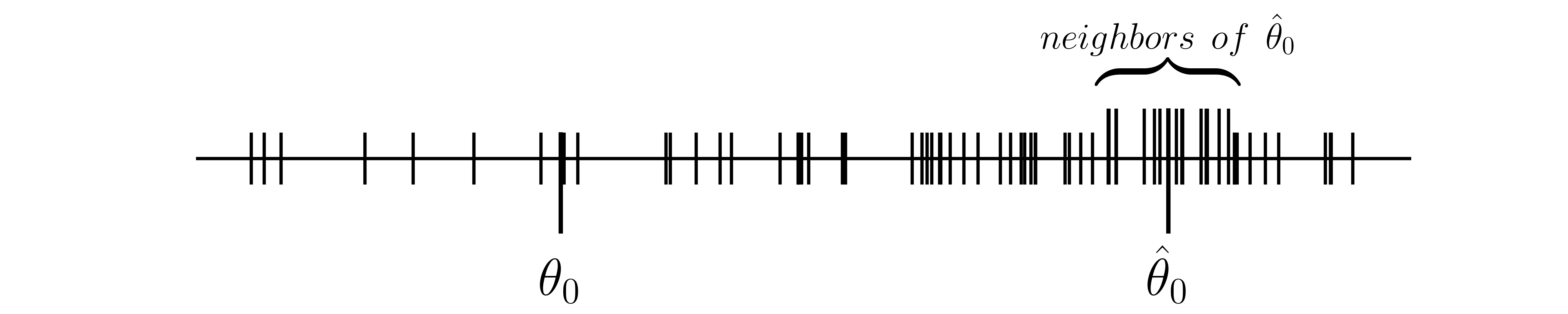
The second part $w_{2}(\hat{\theta}_{k},\hat{\theta}_{0}|\bm{z}_{0})$ measures the similarity between $\hat{\theta}$’s. But unlike $w_{1}$, using a distance measure such as $\mathcal{K}_{2}(\|\hat{\theta}_{k}-\hat{\theta}_{0}\|/b_{2})$ is not a good practice, since it ignores the error in $\hat{\theta}_{0}$ and $\hat{\theta}_{k}$ and $\hat{\theta}_{0}$ may be biased. Note that when $K\rightarrow\infty$ and $b_{2}\rightarrow 0$, the kernel concentrates on a smaller and smaller area adjacent to $\hat{\theta}_{0}$. In this area, aggregating individual $\hat{\theta}_{k}$ will not improve the estimation of $\theta_{0}$. An example of one-dimension case is shown in Figure 3. Vertical bars mark the locations of $\hat{\theta}_{k}$. When $\hat{\theta}_{0}$ is away from its target value $\theta_{0}$, a small bandwidth $b_{2}$ tends to give large weights to individuals in a local region around $\hat{\theta}_{0}$. Aggregating these individual $\hat{\theta}_{k}$ in such a local region will not correct the bias $\hat{\theta}_{0}-\theta_{0}$.

We propose the following weight function that considers the distribution $p(\hat{\theta}|\theta)$ instead of the point estimator $\hat{\theta}$. Specifically, let

Notice that, the posterior distribution of $\theta_{0}$, given $(\hat{\theta}_{0},\bm{z}_{0})$, is

If $\theta_{k}\equiv\theta_{0}$ (hence $\hat{\theta}_{k}$ provides useful information about $\theta_{0}$), then the predictive distribution of $\hat{\theta}_{k}$, given $(\hat{\theta}_{0},\bm{z}_{0})$, is

Thus, the weight function $w_{2}(\hat{\theta}_{k},\hat{\theta}_{0}|\bm{z}_{0},\bm{z}_{k})$ in (5) is the Radon-Nikodym derivative between the predictive distribution $p(\hat{\theta}_{k}|\hat{\theta}_{0},\bm{z}_{0})$ and the sampling distribution $p(\hat{\theta}_{k}|\bm{z}_{k})$. As a result, for any measurable function $h(\cdot)$, we have

That is, the weighted expectation of $h(\hat{\theta}_{k})$ under the sampling distribution $p(\hat{\theta}_{k}|\bm{z}_{k})$ equals to its expectation under the predictive distribution $p(\hat{\theta}_{k}|\hat{\theta}_{0},\bm{z}_{0})$ if $\theta_{k}=\theta_{0}$. This property brings invariance under different sampling distributions. More importantly, it shows that the weighted averages, such as (1) and (2), estimates the expectations under the predictive distribution. This gives the iGroup estimators promising asymptotic properties as we will discuss later in Section 3.

The shape (thin or flat) of the weight $w_{2}(\cdot)$ as a function of $\hat{\theta}_{k}$ does not change with the number of individuals $K$. However, the shape is influenced by the variation (accuracy) of $\hat{\theta}$. The larger the variance of $\hat{\theta}$ is, the flatter the weight function tends to be. If $\hat{\theta}_{k}$ is estimated without any measurement error, the weight $w_{2}(\hat{\theta}_{k},\hat{\theta}_{0}|\bm{z}_{0},\bm{z}_{k})$ is proportional to the indicator function $I_{\{\hat{\theta}_{k}=\hat{\theta}_{0}\}}$. It reduces to the case in which the individual estimator $\hat{\theta}_{0}$ or the individual objective function $M_{0}(\theta)$ is used without grouping.

The weight function $w_{1}(\bm{z}_{k},\bm{z}_{0})$ in (4) can be directly evaluated. Similar to a bandwidth selection problem for kernel smoothing, one can choose the bandwidth $b_{1}$ for $w_{1}(\bm{z}_{k},\bm{z}_{0})$ in (4) by either using the plug-in method (Chiu, 1991) or through cross-validation procedure. The plug-in bandwidth is proportional to $K^{-\frac{1}{d+4}}$ (see Section 3). Also, the leave-one-out cross validation process gives an empirical optimal bandwidth, as discussed in Section 3.6.

The evaluation of the weight function $w_{2}(\hat{\theta}_{k},\hat{\theta}_{0}\mid\bm{z}_{0},\bm{z}_{k})$ in (5) is more complicated, since the conditional probability $p(\hat{\theta}|\bm{z})$ and the integral $\int p(\hat{\theta}_{0}|\theta)p(\hat{\theta}_{k}|\theta)p(\theta|\bm{z}_{0})d\theta$ are unknown as the relationship between $\theta$ and $\bm{z}$ is not explicit. We propose an approximation method to evaluate $w_{2}(\hat{\theta}_{k},\hat{\theta}_{0}\mid\bm{z}_{0},\bm{z}_{k})$ below.

Denote the estimator of $\theta_{k}$ and the observed exogenous variable $\bm{z}_{k}$ as the tuple $(\hat{\theta}_{k},\bm{z}_{k}),k=0,\dots,K.$ To calculate the weight in (5), we treat them as $K+1$ samples from the joint distribution of $(\hat{\theta},\bm{z})$. We use the kernel method to estimate the conditional probability $p(\hat{\theta}\mid\bm{z})$ nonparametrically by

where $\mathcal{K}_{1},\mathcal{K}_{2}$ are two kernel functions with $b_{1}$, $b_{2}$ as the corresponding bandwidths. To estimate the integral in (5), we use the interpretation discussed above that it is the conditional distribution $p(\hat{\theta}_{k}\mid\hat{\theta}_{0},\bm{z}_{0})$ given $\theta_{k}=\theta_{0}$. Hence we need samples from the joint distribution of $(\hat{\theta},\hat{\theta}^{\prime},\bm{z})$ observed from the same individual with parameter $\theta$. However, this is infeasible because in our problem setting, no two individual share the same true parameter $\theta$ and for each individual only one $\hat{\theta}$ is observed. To generate samples from such a distribution, we consider a bootstrap method. Denote $\hat{\theta}^{(1)}_{k}$ and $\hat{\theta}^{(2)}_{k}$ as the two bootstrap estimators for $\theta_{k}$, obtained by re-sampling $\bm{x}_{k}$ with replacement (not applicable when $\bm{x}_{k}$ has few observations). Then $(\hat{\theta}^{(1)}_{k},\hat{\theta}^{(2)}_{k},\bm{z}_{k}),k=0,\dots,K$ is an approximate sample of $(\hat{\theta},\hat{\theta}^{\prime},\bm{z})$, guaranteeing $\hat{\theta}^{(1)}_{k},\hat{\theta}^{(2)}_{k},\bm{z}_{k}$ are generated from the same individual $k$. Therefore the integral can be estimated by

where $\mathcal{K}_{1},\mathcal{K}_{2},\mathcal{K}_{3}$ are three kernel functions with $b_{1},b_{2},b_{3}$ as the corresponding bandwidths. The bandwidths can be selected by either minimizing asymptotic mean integrated squared error (AMISE) or a rule-of-thumb bandwidth estimator. This estimation of the integral is an approximation that requires $K$ to be sufficiently large.

We are interested in making inference about individual 0, with given data information $\mathcal{D}_{x},\mathcal{D}_{z}$ that may include the observations $\bm{x}_{0}$ and $\bm{z}_{0}$ plus information from other relevant individuals. Let $\delta_{0}(\mathcal{D}_{x},\mathcal{D}_{z})$ be a point estimator for $\theta_{0}$, which is constructed with information sets $\mathcal{D}_{x}$ and $\mathcal{D}_{z}$. The iGroup estimator $\hat{\theta}_{0}^{(c)}$ in (1) is such an estimator. Similarly, $\delta_{0}(\mathcal{D}_{x})$ and $\delta_{0}(\mathcal{D}_{z})$ are point estimators constructed solely based on either $\mathcal{D}_{x}$ or $\mathcal{D}_{z}$. Under squared loss, the overall risk of $\delta_{0}$ in estimating $\theta_{0}$ can be decomposed into two nonnegative parts: the expected squared error of $\delta_{0}$ in estimating the corresponding posterior mean and the overall risk of the posterior mean itself, as shown in Proposition 1.

The proof is given in Appendix.

Proposition 1 reveals that the overall risk is minimized by setting $\delta_{0}$ to the corresponding posterior mean under the prior $\pi(\cdot)$, which is the population-level (unknown) distribution for $\theta_{0}$. Throughout this paper, we call the estimator that minimizes the overall risk the target estimator. More specifically, under squared loss and different information sets, we denote the target estimators with

Here, $\ell_{2}$ refers to the squared loss. For the ease of presentation, we also use a simple notation $\Theta_{0}$ to represent one of the Bayes estimators in (6) when its meaning is apparent.

Similarly, for a general loss function $L(\hat{\theta},\theta)$, we define the target estimator as the Bayes estimator that minimizes the expected loss, given the available observation on individual 0 and the prior $\pi(\cdot)$ such that

A similar risk decomposition is demonstrated in Proposition 2 below. Again, for the ease of notation, we simply use $\Theta_{0}$ to represent one of the Bayes estimators in (3.1) when its meaning is apparent.

The proof is given in Appendix.

The target estimator $\Theta_{0}$ as a function of $\bm{x}_{0}$ and $\bm{z}_{0}$ is not directly available, because neither the population distribution $\pi(\theta_{0})$ nor the likelihood function $p(\bm{z}_{0}\mid\theta_{0})$ is explicitly known or assumed. The iGroup estimator $\hat{\theta}_{0}^{(c)}$ in (1) constructed based on observed finite sample $\mathcal{D}_{x},\mathcal{D}_{z}$ is desired to approach the target estimator $\Theta_{0}$ when more and more similar individuals contribute to the estimator $\hat{\theta}_{0}^{(c)}$. See Diaconis and Freedman, 1986 for discussions of target point estimators and target parameters in Bayesian literature.

In the cases when the individual level estimator $\hat{\theta}_{k}$ is not reliable to construct the individual groups, iGroup may be constructed with the exogenous variable $\bm{z}$ only. In this case, the corresponding target estimator is defined as:

where $p(\theta_{0}\mid\bm{z}_{0})\propto p(\bm{z}_{0}\mid\theta_{0})\pi(\theta_{0})$. Although $\bm{x}_{0}$ is not used for grouping and thus does not appear in (8), the data $\mathcal{D}_{x}$ is used in iGroup estimators in (1) and (2).

Recall that the relationship between $\theta_{k}$ and $\bm{\eta}_{k}$ is given by a deterministic relationship

where $g(\cdot)$ is an unknown continuous function. Furthermore, $\bm{z}_{k}$ is a noisy observation of $\bm{\eta}_{k}$. Since $\bm{\eta}$ is a conceptual parameter, we may simply assume that

where the error satisfies $\mathbb{E}(\epsilon_{k})=0$, $\text{Var}(\epsilon_{k})=\sigma_{z}^{2}\bm{\Sigma}_{z}$ with $\|\bm{\Sigma}_{z}\|=1$.

Suppose $\hat{\theta}_{k}$ is an unbiased estimator of $\theta_{k}$. Then, the combined estimator

has all the properties of a conventional kernel smoothing estimator if $\mathcal{K}$ is a standard kernel function. The boundary and asymptotic conditions/assumptions on the weight function $\mathcal{K}$ and the bandwidth $b$ are summarized in Assumption 3.

Theorem 1 follows immediately from consistency theorem on a standard multivariate kernel smoothing estimator (Wasserman, 2010). When the number of individuals $K$ goes to infinity, the bias of $\hat{\theta}_{0}^{(c)}$ with bandwidth $b$ is of order $b^{2}$ and the variance is of order $(b^{d}K)^{-1}$, where $d$ is the dimension of $\bm{z}$ as defined in Assumption 1. In such case, the asymptotic optimal choice of bandwidth that minimizes the mean squared error, $b^{4}+(b^{d}K)^{-1}$, is of order $K^{-1/(d+4)}$, same as a $d$-dimensional kernel smoothing problem.

Another way of combining individuals is aggregating the objective functions as shown in (2). A combined estimator with respect to kernel $\mathcal{K}(\cdot)$ is defined by

The estimator is consistent and has a similar asymptotic performance to a $d$-dimensional kernel smoothing estimator as stated in Theorem 2. This approach is useful especially when $\hat{\theta}_{k}$ is not available, such as in the cases that the number of observations for each individual is less than the number of parameters.

The proof is given in Appendix.

The above theorems suggest that the individualized combined estimator by aggregating either individual estimators $\hat{\theta}_{k}$ or objective functions $M_{k}(\theta)$ would result in an improvement in mean squared error and it shares a similar asymptotic performance as a $d$-dimensional kernel smoothing estimator.

When $\sigma_{z}=0$, $\Theta_{0}(\bm{z}_{0};\ell_{2})=\mathbb{E}_{\pi}[\theta_{0}\mid\bm{z}_{0}]\equiv\theta_{0}$. Hence, estimating $\Theta_{0}$ becomes estimating the unknown function $g(\cdot)$ evaluated at $\bm{z}_{0}$. When $\sigma_{z}>0$, $\Theta_{0}$ and $\theta_{0}$ are in general different. Let $B_{0}$ and $V_{0}$ be the bias and variance of the target estimator $\Theta_{0}(\bm{z}_{0};\ell_{2})$ in estimating $\theta_{0}$ such that

The above bias and variance are defined with respect to a fixed $\theta_{0}$ with random $\bm{z}_{0}$.

The proof is given in Appendix. In the conditional probabilities, $\Theta_{0}=\mathbb{E}_{\pi}[\theta_{0}\mid\bm{z}_{0}]$, as a function of $\bm{z}_{0}$, is considered random under a given $\theta_{0}$.

The bias and variance of $\hat{\theta}_{0}^{(c)}$ in terms of estimating a fixed $\theta_{0}$ can therefore be decomposed into two parts. The first part (the intrinsic part) comes from the bias and variance of estimating $\Theta_{0}[\bm{z}_{0}]$ itself to $\theta_{0}$ and the second part comes from estimating $\Theta_{0}$ nonparametrically. Since $\bm{z}$ is observed with error, this is similar to error in variable problem where certain intrinsic bias cannot be avoided (Fuller, 2009; Carroll et al., 1995; Wansbeek and Meijer, 2000; Bound et al., 2001). Such intrinsic bias and variance are asymptotically linear of $\sigma_{z}^{2}$, which is the noise level of $\bm{z}_{k}$, as shown in Theorem 4. Especially, when $\sigma_{z}^{2}$ is exactly zero, all intrinsic terms vanish, and it reduces to the exact case when $\Theta_{0}=\theta_{0}$.

The proof is given in Appendix.

Research in nonparametric regression with error in variable shows a slower convergence rate to recover the function $\theta_{0}=g(\bm{\eta})$ at any given $\bm{\eta}$ (Stefanski and Carroll, 1990; Fan and Truong, 1993). Our problem is different. We focus on providing a point estimator of $\theta_{0}=g(\bm{\eta}_{0})$ without knowning $\bm{\eta}_{0}$, but its noisy version $\bm{z}_{0}$. Even if we known the function $g(\cdot)$ precisely, $\theta_{0}$ is not known as we do not observe $\eta_{0}$. When considering an individual with fixed but unobserved $(\theta_{0},\bm{\eta}_{0})$, it is difficult to choose an optimal bandwidth by bias-variance optimization with the non-zero intrinsic terms in Theorem 3, because in this case the asymptotic mean squared error $(B_{0}+O_{p}(b^{2}))^{2}+V_{0}+O_{p}((Kb^{d})^{-1})$ may not have a local minimum. However, if we assume the target individual 0 is randomly chosen from the population, the target estimator $\Theta_{0}$ is the estimator that minimizes the overall risk under squared loss, i.e. a Bayes estimator, because it minimizes the squared loss pointwise for any $\bm{z}_{0}$. Furthermore, immediately from Theorem 1, $\hat{\theta}_{0}^{(c)}$ is a consistent estimator for $\Theta_{0}$. The overall performance of $\hat{\theta}_{0}^{(c)}$ for all individuals of the population could be optimized by choosing a proper bandwidth $b$ as stated in the following Theorem 5. It provides a way to optimize the bandwidth globally.

The proof is given in Appendix.

The magnitude of the measurement error of $\bm{z}_{k}$, measured by $\sigma_{z}^{2}$, compared to that of the individual estimation error is crucial for the performance of the iGroup method. The bias and variance of iGroup estimator increase when $\sigma_{z}^{2}$ increases (see Theorem 4). And the asymptotic Bayes risk $R_{0}$ also depends on $\sigma_{z}^{2}$. When iGroup is based on unreliable $\bm{z}$, it could result in a worse estimator compared to the one without any grouping. This phenomenon will be demonstrated in Section 4.
Remark: Results in Theorems 3, 4 and 5 can be generalized to the iGroup estimator $\tilde{\theta}^{(c)}_{0}$, which combines the objective functions, except that the target estimator changes from $\mathbb{E}_{\pi}[\theta|z_{0}]$ is replaced by $\argmin_{\theta}\mathbb{E}_{\pi}[M(\theta)|z_{0}]$. As shown in (19) in the Appendix, $\tilde{\theta}_{0}^{(c)}$ is asymptotically a kernel smoothing estimator with the same bias and variance rates.

In this case, we assume the exogenous variable $\bm{z}$ is not available. Our target estimator is $\Theta_{0}(\bm{x};\ell_{2})=\mathbb{E}_{\pi}[\theta_{0}|\bm{x}_{0}]$ under squared loss and is $\Theta_{0}(\bm{x}_{0};L)=\argmin_{\theta}\mathbb{E}_{\pi}[L(\theta,\theta_{0})\mid\bm{x}_{0}]$ under a general loss function $L$. The iGroup estimation depends solely on $\hat{\theta}$. The weight function (5) used in (1) and (2) now reduces to

where $\pi(\theta)$ corresponds to the unknown distribution of $\theta$ in the whole population. As discussed in Section 2.3, an estimation of this weight function can be achieved by kernel density estimation on the bootstrapped samples $(\hat{\theta}^{(1)}_{k},\hat{\theta}^{(2)}_{k})$.

The weight function (12) is used to aggregated individual unbiased estimators to the posterior mean, and to aggregate objective functions $M:\Omega_{\theta}\times\Omega_{\theta}\rightarrow\mathbb{R}$ to the corresponding Bayes estimator under certain loss function, as shown in Theorems 6 and 7.

The proof is given in Appendix.
For the aggregated estimator (2), suppose the objective function $M:\Omega_{\theta}\times\Omega_{\theta}\rightarrow\mathbb{R}$ used satisfies

where $L$ is non-negative and $L(\theta,\theta)=0$ for all $\theta$, and $C$ is constant with respect to $\theta$. Then $L$ is the loss function corresponding to $M$, under which the target estimator is

Bibliography

• Agrawal et al., (1998) Agrawal, R., Gehrke, J., Gunopulos, D., and Raghavan, P. (1998). Automatic subspace clustering of high dimensional data for data mining applications. SIGMOD Rec., 27(2):94–105.
• Altman, (1992) Altman, N. S. (1992). An introduction to kernel and nearest-neighbor nonparametric regression. The American Statistician, 46(3):175–185.
• Antoniak, (1974) Antoniak, C. E. (1974). Mixtures of dirichlet processes with applications to bayesian nonparametric problems. The Annals of Statistics, 2(6):1152–1174.
• Binder, (1978) Binder, D. A. (1978). Bayesian cluster analysis. Biometrika, 65(1):31–38.
• Bound et al., (2001) Bound, J., Brown, C., and Mathiowetz, N. (2001). Measurement error in survey data. In Handbook of Econometrics, volume 5, pages 3705–3843. Elsevier.
• Carroll et al., (1995) Carroll, R., Ruppert, D., and Stefanski, L. (1995). Nonlinear measurement error models. Monographs on Statistics and Applied Probability, 63.
• Chiu, (1991) Chiu, S.-T. (1991). Bandwidth selection for kernel density estimation. The Annals of Statistics, 19(4):1883–1905.
• Collins and Varmus, (2015) Collins, F. S. and Varmus, H. (2015). A new initiative on precision medicine. New England Journal of Medicine, 372(9):793–795.
• Diaconis and Freedman, (1986) Diaconis, P. and Freedman, D. (1986). On the consistency of bayes estimates. The Annals of Statistics, 14(1):1–26.
• Duda and Hart, (1973) Duda, R. O. and Hart, P. E. (1973). Pattern Classification and Scene Analysis. John Willey & Sons, New York.
• Fama and French, (1993) Fama, E. F. and French, K. R. (1993). Common risk factors in the returns on stocks and bonds. Journal of Financial Economics, 33(1):3–56.
• Fan and Truong, (1993) Fan, J. and Truong, Y. K. (1993). Nonparametric regression with errors in variables. The Annals of Statistics, 21(4):1900–1925.
• Ferguson, (1973) Ferguson, T. S. (1973). A bayesian analysis of some nonparametric problems. The Annals of Statistics, 1(2):209–230.
• Figueiredo and Jain, (2000) Figueiredo, M. A. T. and Jain, A. K. (2000). Unsupervised learning of finite mixture models. IEEE Transaction on Pattern Analysis and Machine Intelligence, 24:381–396.
• Fuller, (2009) Fuller, W. A. (2009). Measurement error models, volume 305. John Wiley & Sons.
• Gan et al., (2007) Gan, G., Ma, C., and Wu, J. (2007). Data Clustering: Theory, Algorithms, and Applications, volume 20. Society for Industrial and Applied Mathematics.
• Hall et al., (2008) Hall, P., Park, B. U., and Samworth, R. J. (2008). Choice of neighbor order in nearest-neighbor classification. The Annals of Statistics, 36(5):2135–2152.
• Jain, (2010) Jain, A. K. (2010). Data clustering: 50 years beyond k-means. Pattern Recognition Letters, 31(8):651–666.
• Jain et al., (1999) Jain, A. K., Murty, M. N., and Flynn, P. J. (1999). Data clustering: a review. ACM Computing Surveys (CSUR), 31(3):264–323.
• Juang, (1984) Juang, B.-H. (1984). On the hidden markov model and dynamic time warping for speech recognition - a unified view. AT&T Bell Laboratories Technical Journal, 63(7):1213–1243.
• Koenig et al., (2008) Koenig, L. L., Lucero, J. C., and Perlman, E. (2008). Speech production variability in fricatives of children and adults: Results of functional data analysis. The Journal of the Acoustical Society of America, 124(5):3158–3170.
• Liao, (2005) Liao, T. W. (2005). Clustering of time series data - a survey. Pattern Recognition, 38(11):1857–1874.
• Lindsay, (1995) Lindsay, B. G. (1995). Mixture models: Theory, geometry and applications. NSF-CBMS Regional Conference Series in Probability and Statistics, 5:i–163.
• Liu and Meng, (2016) Liu, K. and Meng, X. L. (2016). There is individualized treatment. why not individualized inference? Annual Review of Statistics and Its Application, 3:79–111.
• Lo, (1984) Lo, A. Y. (1984). On a class of bayesian nonparametric estimates: I. density estimates. The Annals of Statistics, 12(1):351–357.
• Nakagawa and Nakanishi, (1988) Nakagawa, S. and Nakanishi, H. (1988). Speaker-independent english consonant and japanese word recognition by a stochastic dynamic time warping method. IETE Journal of Research, 34(1):87–95.
• Ng and Han, (1994) Ng, R. T. and Han, J. (1994). Efficient and effective clustering methods for spatial data mining. In Proceedings of the 20th International Conference on Very Large Data Bases, VLDB ’94, pages 144–155. Morgan Kaufmann Publishers Inc.
• Qian and Murphy, (2011) Qian, M. and Murphy, S. A. (2011). Performance guarantees for individualized treatment rules. The Annals of Statistics, 39(2):1180.
• Robbins, (1956) Robbins, H. (1956). An empirical bayes approach to statistics. In Proceedings of the Third Berkeley Symposium on Mathematical Statistics and Probability, Volume 1: Contributions to the Theory of Statistics, pages 157–163. University of California Press.
• Sakoe and Chiba, (1978) Sakoe, H. and Chiba, S. (1978). Dynamic programming algorithm optimization for spoken word recognition. IEEE Transactions on Acoustics, Speech, and Signal Processing, 26(1):43–49.
• Shen et al., (2018) Shen, J., Liu, R., and Xie, M. (2018). ii-Fusion: Individualized fusion learning. manuscript.
• Stefanski and Carroll, (1990) Stefanski, L. A. and Carroll, R. J. (1990). Deconvolving kernel density estimators. Statistics, 21(2):169–184.
• Teh et al., (2005) Teh, Y. W., Jordan, M. I., Beal, M. J., and Blei, D. M. (2005). Sharing clusters among related groups: Hierarchical dirichlet processes. In Advances in Neural Information Processing Systems 17, pages 1385–1392. MIT Press.
• Van der Vaart, (2000) Van der Vaart, A. W. (2000). Asymptotic statistics, volume 3. Cambridge University Press.
• Wang et al., (2007) Wang, R., Lagakos, S. W., Ware, J. H., Hunter, D. J., and Drazen, J. M. (2007). Statistics in medicine—reporting of subgroup analyses in clinical trials. New England Journal of Medicine, 357(21):2189–2194.
• Wansbeek and Meijer, (2000) Wansbeek, T. J. and Meijer, E. (2000). Measurement error and latent variables in econometrics, volume 37. North-Holland.
• Wasserman, (2010) Wasserman, L. (2010). All of Nonparametric Statistics. Springer Publishing Company, Incorporated.
• Xu and Wunsch, (2005) Xu, R. and Wunsch, D. (2005). Survey of clustering algorithms. IEEE Transactions on Neural Networks, 16(3):645–678.
• Yang et al., (2012) Yang, J., Miescke, K., and McCullagh, P. (2012). Classification based on a permanental process with cyclic approximation. Biometrika, 99(4):775–786.
• Zhao et al., (2012) Zhao, Y., Zeng, D., Rush, A. J., and Kosorok, M. R. (2012). Estimating individualized treatment rules using outcome weighted learning. Journal of the American Statistical Association, 107(499):1106–1118.
Proof of Theorem 2
We prove the consistency first. Define
ψk​(θ)\displaystyle\psi_{k}(\theta) =∂∂θ​Mk​(θ),\displaystyle=\dfrac{\partial}{\partial\theta}M_{k}(\theta),
ΨK​(θ)\displaystyle\Psi_{K}(\theta) =∑k=0K𝒦⁡(‖𝒛k−𝒛0‖b)​ψk​(θ)∑k=0K𝒦⁡(‖𝒛k−𝒛0‖b),\displaystyle=\dfrac{\sum_{k=0}^{K}\mathcal{K}\left(\dfrac{\|\bm{z}_{k}-\bm{z}_{0}\|}{b}\right)\psi_{k}(\theta)}{\sum_{k=0}^{K}\mathcal{K}\left(\dfrac{\|\bm{z}_{k}-\bm{z}_{0}\|}{b}\right)},
Ψ⁡(θ)\displaystyle\Psi(\theta) =𝔼𝒙|𝒛0​ψ𝒙​(θ).\displaystyle=\mathbb{E}_{\bm{x}|\bm{z}_{0}}\psi_{\bm{x}}(\theta).
For any given θ\theta, ΨK​(θ)\Psi_{K}(\theta) is a kernel smoothing estimator for 𝔼𝒙|𝒛0​[ψ𝒙​(θ)]=Ψ⁡(θ)\mathbb{E}_{\bm{x}|\bm{z}_{0}}[\psi_{\bm{x}}(\theta)]=\Psi(\theta). Hence ΨK​(θ)→Ψ⁡(θ)\Psi_{K}(\theta)\rightarrow\Psi(\theta) in probability for any given θ\theta, provided 𝔼𝒙|𝒛​[ψ𝒙​(θ)]\mathbb{E}_{\bm{x}|\bm{z}}[\psi_{\bm{x}}(\theta)] continuous at 𝒛0\bm{z}_{0} (Wasserman, 2010). Due to the assumption that Mk​(θ)M_{k}(\theta) is convex and second-order differentiable, ψk​(θ)\psi_{k}(\theta) is a non-decreasing function for any 𝒙k\bm{x}_{k}. Therefore, both ΨK\Psi_{K} and Ψ\Psi are non-decreasing and continuous. By assumption, Θ0\Theta_{0} is the unique root of Ψ⁡(θ)\Psi(\theta). Let θK∗\theta^{*}_{K} be such a point that ΨK​(θK∗)=0\Psi_{K}(\theta^{*}_{K})=0. θK∗\theta^{*}_{K} may not be unique and may not even exist for small KK. For any ϵ>0\epsilon>0, it is immediate that Ψ⁡(Θ0−ϵ)<0<Ψ⁡(Θ0+ϵ)\Psi(\Theta_{0}-\epsilon)<0<\Psi(\Theta_{0}+\epsilon) and by the pointwise convergence in probability of ΨK\Psi_{K}, we have
P[|ΨK(Θ0−ϵ)−Ψ(Θ0−ϵ)|⩽12|Ψ(Θ0−ϵ)|]\displaystyle P\left[\left|\Psi_{K}(\Theta_{0}-\epsilon)-\Psi(\Theta_{0}-\epsilon)\right|\leqslant\dfrac{1}{2}\left|\Psi(\Theta_{0}-\epsilon)\right|\right] ⟶1,\displaystyle\longrightarrow 1,
P[|ΨK(Θ0+ϵ)−Ψ(Θ0+ϵ)|⩽12|Ψ(Θ0+ϵ)|]\displaystyle P\left[\left|\Psi_{K}(\Theta_{0}+\epsilon)-\Psi(\Theta_{0}+\epsilon)\right|\leqslant\dfrac{1}{2}\left|\Psi(\Theta_{0}+\epsilon)\right|\right] ⟶1.\displaystyle\longrightarrow 1.
Therefore,
P⁡[|ΨK​(Θ0−ϵ)−Ψ⁡(Θ0−ϵ)|⩽12​|Ψ⁡(Θ0−ϵ)|,|ΨK​(Θ0+ϵ)−Ψ⁡(Θ0+ϵ)|⩽12​|Ψ⁡(Θ0+ϵ)|]⟶1.P\left[\left|\Psi_{K}(\Theta_{0}-\epsilon)-\Psi(\Theta_{0}-\epsilon)\right|\leqslant\dfrac{1}{2}\left|\Psi(\Theta_{0}-\epsilon)\right|,\left|\Psi_{K}(\Theta_{0}+\epsilon)-\Psi(\Theta_{0}+\epsilon)\right|\leqslant\dfrac{1}{2}\left|\Psi(\Theta_{0}+\epsilon)\right|\right]\longrightarrow 1.
The event in the probability implies that ΨK​(Θ0−ϵ)<0<ΨK​(Θ0+ϵ)\Psi_{K}(\Theta_{0}-\epsilon)<0<\Psi_{K}(\Theta_{0}+\epsilon), which further implies the existence of θK∗\theta_{K}^{*} in (Θ0−ϵ,Θ0+ϵ)(\Theta_{0}-\epsilon,\Theta_{0}+\epsilon) by continuity of ΨK\Psi_{K}. Hence
P⁡[|ΨK​(Θ0−ϵ)−Ψ⁡(Θ0−ϵ)|⩽12​|Ψ⁡(Θ0−ϵ)|,|ΨK​(Θ0+ϵ)−Ψ⁡(Θ0+ϵ)|⩽12​|Ψ⁡(Θ0+ϵ)|]\displaystyle P\left[\left|\Psi_{K}(\Theta_{0}-\epsilon)-\Psi(\Theta_{0}-\epsilon)\right|\leqslant\dfrac{1}{2}\left|\Psi(\Theta_{0}-\epsilon)\right|,\left|\Psi_{K}(\Theta_{0}+\epsilon)-\Psi(\Theta_{0}+\epsilon)\right|\leqslant\dfrac{1}{2}\left|\Psi(\Theta_{0}+\epsilon)\right|\right]
⩽\displaystyle\leqslant P[ΨK(Θ0−ϵ)<0<ΨK(Θ0+ϵ)]\displaystyle P\left[\Psi_{K}(\Theta_{0}-\epsilon)<0<\Psi_{K}(\Theta_{0}+\epsilon)\right]
⩽\displaystyle\leqslant P[Θ0−ϵ<θK∗<Θ0+ϵ].\displaystyle P\left[\Theta_{0}-\epsilon<\theta_{K}^{*}<\Theta_{0}+\epsilon\right].
Since the first term converges to 1, the last term converges to 1 as well. Note that when θ~0(c)\tilde{\theta}_{0}^{(c)} exists, it equals θK∗\theta_{K}^{*}. The consistency of θ~0(c)\tilde{\theta}_{0}^{(c)} is proved.
With θ~0(c)⟶θ0\tilde{\theta}_{0}^{(c)}\longrightarrow\theta_{0} in probability, it is reasonable to expand ΨK​(θ~0(c))\Psi_{K}(\tilde{\theta}_{0}^{(c)}) at Θ0\Theta_{0}.
∑k=0K𝒦⁡(‖𝒛k−𝒛0‖b)​ψk​(Θ0)+(θ~(c)−Θ0)​∑k=0K𝒦⁡(‖𝒛k−𝒛0‖b)​ψk′​(Θ0)\displaystyle\sum_{k=0}^{K}\mathcal{K}\left(\dfrac{\|\bm{z}_{k}-\bm{z}_{0}\|}{b}\right)\psi_{k}(\Theta_{0})+(\tilde{\theta}^{(c)}-\Theta_{0})\sum_{k=0}^{K}\mathcal{K}\left(\dfrac{\|\bm{z}_{k}-\bm{z}_{0}\|}{b}\right)\psi^{\prime}_{k}(\Theta_{0})
+∑k=0K𝒦(‖𝒛k−𝒛0‖b)O((θ~0(c)−Θ0)2)=0.\displaystyle+\sum_{k=0}^{K}\mathcal{K}\left(\dfrac{\|\bm{z}_{k}-\bm{z}_{0}\|}{b}\right)O((\tilde{\theta}^{(c)}_{0}-\Theta_{0})^{2})=0.
Now we have
θ~0(c)−Θ0=−1K+1​∑k=0K𝒦⁡(‖𝒛k−𝒛0‖b)​ψk​(Θ0)1K+1​∑k=0K𝒦⁡(‖𝒛k−𝒛0‖b)​ψk′​(Θ0)+O⁡(θ^0(c)−Θ0).\tilde{\theta}^{(c)}_{0}-\Theta_{0}=-\dfrac{\dfrac{1}{K+1}\sum_{k=0}^{K}\mathcal{K}\left(\dfrac{\|\bm{z}_{k}-\bm{z}_{0}\|}{b}\right)\psi_{k}(\Theta_{0})}{\dfrac{1}{K+1}\sum_{k=0}^{K}\mathcal{K}\left(\dfrac{\|\bm{z}_{k}-\bm{z}_{0}\|}{b}\right)\psi^{\prime}_{k}(\Theta_{0})+O(\hat{\theta}^{(c)}_{0}-\Theta_{0})}. (19)
Consider K→∞K\rightarrow\infty. On one hand, the numerator is a kernel smoothing estimator for 𝔼𝒙|𝒛0​[ψ𝒙​(Θ0)]=0\mathbb{E}_{\bm{x}|\bm{z}_{0}}[\psi_{\bm{x}}(\Theta_{0})]=0 up to a normalizing constant. On the other hand, the denominator is a similar kernel smoothing estimator for 𝔼𝒙|𝒛0​ψ𝒙′​(Θ0)\mathbb{E}_{\bm{x}|\bm{z}_{0}}\psi^{\prime}_{\bm{x}}(\Theta_{0}). By Slutsky’s theorem, their ratio has a similar asymptotic distribution to the numerator kernel smoothing estimator up to a constant factor of 𝔼𝒙|𝒛0​ψ𝒙′​(Θ0)\mathbb{E}_{\bm{x}|\bm{z}_{0}}\psi^{\prime}_{\bm{x}}(\Theta_{0}). Therefore, θ~0(c)\tilde{\theta}_{0}^{(c)} has an asymptotic bias Op​(b2)O_{p}(b^{2}) and an asymptotic variance Op​(1/K​bd)O_{p}(1/Kb^{d}) (Wasserman, 2010). Hence, the optimal choice of bandwidth in a bias-variance optimization scheme is b^≍K−1/(d+4)\hat{b}\asymp K^{-1/(d+4)} and the optimal MSE is of order K−4/(d+4)K^{-4/(d+4)}.
Proof of Theorem 3
In this case, θ0\theta_{0} is assumed to be fixed, and θ^0(c)\hat{\theta}_{0}^{(c)} is a standard kernel smoothing estimator for 𝔼π​[θ0|𝒛0]=Θ0\mathbb{E}_{\pi}[\theta_{0}|\bm{z}_{0}]=\Theta_{0}. By following the asymptotic property of a standard kernel smoothing estimator, we have
𝔼⁡[θ^0(c)|𝒛0]=Θ0+Op​(b2)​ and ​V​a​r​[θ^0(c)|𝒛0]=Op​(1K​db).\displaystyle\mathbb{E}[\hat{\theta}_{0}^{(c)}|\bm{z}_{0}]=\Theta_{0}+O_{p}(b^{2})\text{ and }Var[\hat{\theta}_{0}^{(c)}|\bm{z}_{0}]=O_{p}\left(\dfrac{1}{Kd^{b}}\right).
Therefore, we have
𝔼θ0​[θ^0(c)]=𝔼θ0​[Θ0]+Op​(b2),\displaystyle\mathbb{E}_{\theta_{0}}[\hat{\theta}_{0}^{(c)}]=\mathbb{E}_{\theta_{0}}[\Theta_{0}]+O_{p}(b^{2}),
V​a​rθ0​[θ^0(c)]=V​a​rθ0​[𝔼⁡[θ^0(c)|𝒛0]]+𝔼θ0​[V​a​r​[θ^0(c)|𝒛0]]=V​a​rθ0​[Θ0]+Op​(1K​db).\displaystyle Var_{\theta_{0}}[\hat{\theta}_{0}^{(c)}]=Var_{\theta_{0}}[\mathbb{E}[\hat{\theta}_{0}^{(c)}|\bm{z}_{0}]]+\mathbb{E}_{\theta_{0}}[Var[\hat{\theta}_{0}^{(c)}|\bm{z}_{0}]]=Var_{\theta_{0}}[\Theta_{0}]+O_{p}\left(\dfrac{1}{Kd^{b}}\right).
Proof of Theorem 4
We first prove the following lemma, which would be used in the proof of Theorem 4.
Lemma 1.
Suppose the random vector ξ\xi has a pdf pξp_{\xi} and has zero mean, finite variance and finite higher moments such that
𝔼​ξ=0,Var​(ξ)=σ2​𝚺,‖𝚺‖=1.\mathbb{E}\xi=0,\quad\text{Var}(\xi)=\sigma^{2}\bm{\Sigma},\quad\|\bm{\Sigma}\|=1.
Then for any second-order partially differentiable function ff, we have
∫f⁡(𝒙+t)​pξ​(t)​𝑑t=f⁡(𝒙)+12​σ2​tr⁡[∇2f​(𝒙)​𝚺]+o⁡(σ2),\int f(\bm{x}+t)p_{\xi}(t)dt=f(\bm{x})+\dfrac{1}{2}\sigma^{2}\tr[\nabla^{2}f(\bm{x})\bm{\Sigma}]+o(\sigma^{2}),
when σ2→0\sigma^{2}\rightarrow 0.
Proof.
Let ξ1=ξ/σ\xi_{1}=\xi/\sigma, then 𝔼⁡(ξ1)=0\mathbb{E}(\xi_{1})=0 and Var​(ξ1)=𝚺\text{Var}(\xi_{1})=\bm{\Sigma}. Hence
∫f⁡(𝒙+t)​pξ​(t)​𝑑t\displaystyle\int f(\bm{x}+t)p_{\xi}(t)dt =∫f⁡(𝒙+σ​s)​pξ1​(s)​𝑑s\displaystyle=\int f(\bm{x}+\sigma s)p_{\xi_{1}}(s)ds
=∫[f⁡(𝒙)+σ​sT​[∇f​(𝒙)]+12​σ2​sT​[∇2f​(x)]​s+o⁡(σ2)]​pξ1​(s)​𝑑s\displaystyle=\int\left[f(\bm{x})+\sigma s^{T}[\nabla f(\bm{x})]+\dfrac{1}{2}\sigma^{2}s^{T}[\nabla^{2}f(x)]s+o(\sigma^{2})\right]p_{\xi_{1}}(s)ds
=f⁡(𝒙)+12​σ2​∫sT​[∇2f​(𝒙)]​s​pξ1​(s)​𝑑s+o⁡(σ2)\displaystyle=f(\bm{x})+\dfrac{1}{2}\sigma^{2}\int s^{T}[\nabla^{2}f(\bm{x})]sp_{\xi_{1}}(s)ds+o(\sigma^{2})
=f⁡(𝒙)+12​σ2​tr⁡[∇2f​(𝒙)​𝚺]+o⁡(σ2).\displaystyle=f(\bm{x})+\dfrac{1}{2}\sigma^{2}\tr[\nabla^{2}f(\bm{x})\bm{\Sigma}]+o(\sigma^{2}).
∎
Now we prove Theorem 4. Let π¯​()\bar{\pi}() be the population distribution for 𝜼\bm{\eta}. Since θ=g⁡(𝜼)\theta=g(\bm{\eta}), we have
𝔼π​[θ0|𝒛0]\displaystyle\mathbb{E}_{\pi}[\theta_{0}|\bm{z}_{0}] =∫g⁡(𝜼)​p​(𝒛0|𝜼)​π¯​(𝜼)​𝑑𝜼∫p⁡(𝒛0|𝜼)​π¯​(𝜼)​𝑑𝜼\displaystyle=\dfrac{\int g(\bm{\eta})p(\bm{z}_{0}|\bm{\eta})\bar{\pi}(\bm{\eta})d\bm{\eta}}{\int p(\bm{z}_{0}|\bm{\eta})\bar{\pi}(\bm{\eta})d\bm{\eta}}
=(g​π¯)​(𝒛0)+12​σz2​tr⁡[∇2(g​π¯)​(𝒛0)​𝚺z]+o⁡(σz2)π¯​(𝒛0)+12​σz2​tr⁡[∇2π¯​(𝒛0)​𝚺z]+o⁡(σz2)\displaystyle=\dfrac{(g\bar{\pi})(\bm{z}_{0})+\dfrac{1}{2}\sigma_{z}^{2}\tr[\nabla^{2}(g\bar{\pi})(\bm{z}_{0})\bm{\Sigma}_{z}]+o(\sigma_{z}^{2})}{\bar{\pi}(\bm{z}_{0})+\dfrac{1}{2}\sigma_{z}^{2}\tr[\nabla^{2}\bar{\pi}(\bm{z}_{0})\bm{\Sigma}_{z}]+o(\sigma_{z}^{2})}
=(g​π¯)​(𝒛0)+12​σz2​tr⁡[∇2(g​π¯)​(𝒛0)​𝚺z]+o⁡(σz2)π¯​(𝒛0)​[1−12​σz2​tr⁡[∇2π¯​(𝒛0)​𝚺z]π¯​(𝒛0)+o⁡(σz2)]\displaystyle=\dfrac{(g\bar{\pi})(\bm{z}_{0})+\dfrac{1}{2}\sigma_{z}^{2}\tr[\nabla^{2}(g\bar{\pi})(\bm{z}_{0})\bm{\Sigma}_{z}]+o(\sigma_{z}^{2})}{\bar{\pi}(\bm{z}_{0})}\left[1-\dfrac{1}{2}\sigma_{z}^{2}\dfrac{\tr[\nabla^{2}\bar{\pi}(\bm{z}_{0})\bm{\Sigma}_{z}]}{\bar{\pi}(\bm{z}_{0})}+o(\sigma_{z}^{2})\right]
=g⁡(𝒛0)+σz22​π¯​(𝒛0)​(tr⁡[∇2(g​π¯)​(𝒛0)​𝚺z]−g⁡(𝒛0)​tr​[∇2π¯​(𝒛0)​𝚺z])+o⁡(σz2)\displaystyle=g(\bm{z}_{0})+\dfrac{\sigma_{z}^{2}}{2\bar{\pi}(\bm{z}_{0})}\left(\tr[\nabla^{2}(g\bar{\pi})(\bm{z}_{0})\bm{\Sigma}_{z}]-g(\bm{z}_{0})\tr[\nabla^{2}\bar{\pi}(\bm{z}_{0})\bm{\Sigma}_{z}]\right)+o(\sigma_{z}^{2})
=g⁡(𝒛0)+σz2​(tr⁡[∇2g​(𝒛0)​𝚺z]2+tr[∇π¯(𝒛0)T𝚺z∇g(𝒛0)]π¯​(𝒛0))+o⁡(σz2).\displaystyle=g(\bm{z}_{0})+\sigma_{z}^{2}\left(\dfrac{\tr[\nabla^{2}g(\bm{z}_{0})\bm{\Sigma}_{z}]}{2}+\dfrac{\tr[\nabla\bar{\pi}(\bm{z}_{0})^{T}\bm{\Sigma}_{z}\nabla g(\bm{z}_{0})]}{\bar{\pi}(\bm{z}_{0})}\right)+o(\sigma_{z}^{2}).
Thus, the bias is
𝔼θ0​[𝔼π​[g⁡(𝜼)|𝒛0]]−g⁡(𝜼0)\displaystyle\mathbb{E}_{\theta_{0}}[\mathbb{E}_{\pi}[g(\bm{\eta})|\bm{z}_{0}]]-g(\bm{\eta}_{0}) =∫𝔼π​[g⁡(𝜼)|𝒛0]​p​(𝒛0|𝜼0)​d​𝒛0−g⁡(𝜼0)\displaystyle=\int\mathbb{E}_{\pi}[g(\bm{\eta})|\bm{z}_{0}]p(\bm{z}_{0}|\bm{\eta}_{0})d\bm{z}_{0}-g(\bm{\eta}_{0})
=∫(g⁡(𝒛0)+σz2​(tr⁡[∇2g​(𝒛0)​𝚺z]2+tr[∇π¯(𝒛0)T𝚺z∇g(𝒛0)]π¯​(𝒛0))+o⁡(σz2))​p​(𝒛0|𝜼0)​d​𝒛0−g⁡(𝜼0)\displaystyle=\int\left(g(\bm{z}_{0})+\sigma_{z}^{2}\left(\dfrac{\tr[\nabla^{2}g(\bm{z}_{0})\bm{\Sigma}_{z}]}{2}+\dfrac{\tr[\nabla\bar{\pi}(\bm{z}_{0})^{T}\bm{\Sigma}_{z}\nabla g(\bm{z}_{0})]}{\bar{\pi}(\bm{z}_{0})}\right)+o(\sigma_{z}^{2})\right)p(\bm{z}_{0}|\bm{\eta}_{0})d\bm{z}_{0}-g(\bm{\eta}_{0})
=g⁡(𝜼0)+σz2​(tr⁡[∇2g​(𝜼0)​𝚺z]2+tr[∇π¯(𝜼0)T𝚺z∇g(𝜼0)]π¯​(𝜼0))\displaystyle=g(\bm{\eta}_{0})+\sigma_{z}^{2}\left(\dfrac{\tr[\nabla^{2}g(\bm{\eta}_{0})\bm{\Sigma}_{z}]}{2}+\dfrac{\tr[\nabla\bar{\pi}(\bm{\eta}_{0})^{T}\bm{\Sigma}_{z}\nabla g(\bm{\eta}_{0})]}{\bar{\pi}(\bm{\eta}_{0})}\right)
+12​σz2​tr⁡[∇2g​(𝜼0)​𝚺z]+o⁡(σz2)−g⁡(𝜼0)\displaystyle\ \ +\dfrac{1}{2}\sigma_{z}^{2}\tr[\nabla^{2}g(\bm{\eta}_{0})\bm{\Sigma}_{z}]+o(\sigma_{z}^{2})-g(\bm{\eta}_{0})
=σz2​(tr⁡[∇2g​(𝜼0)​𝚺z]+tr[∇π¯(𝜼0)T𝚺z∇g(𝜼0)]π¯​(𝜼0))+o⁡(σz2)\displaystyle=\sigma_{z}^{2}\left(\tr[\nabla^{2}g(\bm{\eta}_{0})\bm{\Sigma}_{z}]+\dfrac{\tr[\nabla\bar{\pi}(\bm{\eta}_{0})^{T}\bm{\Sigma}_{z}\nabla g(\bm{\eta}_{0})]}{\bar{\pi}(\bm{\eta}_{0})}\right)+o(\sigma_{z}^{2})
≍σz2.\displaystyle\asymp\sigma_{z}^{2}.
On the other hand,
(𝔼π​[g⁡(𝜼)|𝒛0])2=g2​(𝒛0)+σz2​[g​tr⁡[∇2g​(𝒛0)​𝚺z]+2gtr[∇π¯(𝒛0)T𝚺z∇g(𝒛0)]π¯​(𝒛0)]+o⁡(σz2),\left(\mathbb{E}_{\pi}[g(\bm{\eta})|\bm{z}_{0}]\right)^{2}=g^{2}(\bm{z}_{0})+\sigma_{z}^{2}\left[g\tr[\nabla^{2}g(\bm{z}_{0})\bm{\Sigma}_{z}]+\dfrac{2g\tr[\nabla\bar{\pi}(\bm{z}_{0})^{T}\bm{\Sigma}_{z}\nabla g(\bm{z}_{0})]}{\bar{\pi}(\bm{z}_{0})}\right]+o(\sigma_{z}^{2}),
hence
𝔼θ0​[(𝔼π​[g⁡(𝜼)|𝒛0])2]\displaystyle\mathbb{E}_{\theta_{0}}\left[\left(\mathbb{E}_{\pi}[g(\bm{\eta})|\bm{z}_{0}]\right)^{2}\right] =∫(𝔼π​[g⁡(𝜼)|𝒛0])2​p​(𝒛0|𝜼0)​d​𝒛0\displaystyle=\int\left(\mathbb{E}_{\pi}[g(\bm{\eta})|\bm{z}_{0}]\right)^{2}p(\bm{z}_{0}|\bm{\eta}_{0})d\bm{z}_{0}
=∫(g2​(𝒛0)+σz2​[g​tr⁡[∇2g​(𝒛0)​𝚺z]+2gtr[∇π¯(𝒛0)T𝚺z∇g(𝒛0)]π¯​(𝒛0)]+o⁡(σz2))​p​(𝒛0|𝜼0)​d​𝒛0\displaystyle=\int\left(g^{2}(\bm{z}_{0})+\sigma_{z}^{2}\left[g\tr[\nabla^{2}g(\bm{z}_{0})\bm{\Sigma}_{z}]+\dfrac{2g\tr[\nabla\bar{\pi}(\bm{z}_{0})^{T}\bm{\Sigma}_{z}\nabla g(\bm{z}_{0})]}{\bar{\pi}(\bm{z}_{0})}\right]+o(\sigma_{z}^{2})\right)p(\bm{z}_{0}|\bm{\eta}_{0})d\bm{z}_{0}
=g2​(𝜼0)+σz2​[g​tr⁡[∇2g​(𝜼0)​𝚺z]+2gtr[∇π¯(𝜼0)T𝚺z∇g(𝜼0)]π¯​(𝜼0)]+12​σz2​tr⁡[∇2(g2)​(𝜼0)​𝚺z]+o⁡(σz2)\displaystyle=g^{2}(\bm{\eta}_{0})+\sigma_{z}^{2}\left[g\tr[\nabla^{2}g(\bm{\eta}_{0})\bm{\Sigma}_{z}]+\dfrac{2g\tr[\nabla\bar{\pi}(\bm{\eta}_{0})^{T}\bm{\Sigma}_{z}\nabla g(\bm{\eta}_{0})]}{\bar{\pi}(\bm{\eta}_{0})}\right]+\dfrac{1}{2}\sigma_{z}^{2}\tr[\nabla^{2}(g^{2})(\bm{\eta}_{0})\bm{\Sigma}_{z}]+o(\sigma_{z}^{2})
=g2(𝜼0)+σz2[2gtr[∇2g(𝜼0)𝚺z]+2gtr[∇π¯(𝜼0)T𝚺z∇g(𝜼0)]π¯​(𝜼0)+tr[∇g(𝜼0)T𝚺z∇g(𝜼0)]]+o(σz2).\displaystyle=g^{2}(\bm{\eta}_{0})+\sigma_{z}^{2}\left[2g\tr[\nabla^{2}g(\bm{\eta}_{0})\bm{\Sigma}_{z}]+\dfrac{2g\tr[\nabla\bar{\pi}(\bm{\eta}_{0})^{T}\bm{\Sigma}_{z}\nabla g(\bm{\eta}_{0})]}{\bar{\pi}(\bm{\eta}_{0})}+\tr[\nabla g(\bm{\eta}_{0})^{T}\bm{\Sigma}_{z}\nabla g(\bm{\eta}_{0})]\right]+o(\sigma_{z}^{2}).
Therefore, the variance is
Varθ0​[𝔼π​[g⁡(𝜼)|𝒛0]]\displaystyle\text{Var}_{\theta_{0}}[\mathbb{E}_{\pi}[g(\bm{\eta})|\bm{z}_{0}]] =𝔼θ0​[(𝔼π​[g⁡(𝜼)|𝒛0])2]−[𝔼θ0​[𝔼π​[g⁡(𝜼)|𝒛0]|𝜼0]]2\displaystyle=\mathbb{E}_{\theta_{0}}\left[\left(\mathbb{E}_{\pi}[g(\bm{\eta})|\bm{z}_{0}]\right)^{2}\right]-\left[\mathbb{E}_{\theta_{0}}[\mathbb{E}_{\pi}[g(\bm{\eta})|\bm{z}_{0}]|\bm{\eta}_{0}]\right]^{2}
=σz2∇g(𝜼0)T𝚺z∇g(𝜼0)+o(σz2)\displaystyle=\sigma_{z}^{2}\nabla g(\bm{\eta}_{0})^{T}\bm{\Sigma}_{z}\nabla g(\bm{\eta}_{0})+o(\sigma_{z}^{2})
Proof of Theorem 5
From Theorem 3, we have
𝔼θ0​[(θ^0(c)−θ0)2]=B02+2​B0​Op​(b2)+Op​(b4)+V0+Op​(1K​db).\mathbb{E}_{\theta_{0}}[(\hat{\theta}_{0}^{(c)}-\theta_{0})^{2}]=B_{0}^{2}+2B_{0}O_{p}(b^{2})+O_{p}(b^{4})+V_{0}+O_{p}\left(\dfrac{1}{Kd^{b}}\right).
𝔼⁡[B0]\displaystyle\mathbb{E}[B_{0}] =𝔼⁡[𝔼θ0​[𝔼π​[g⁡(𝜼)|𝒛0]]−g⁡(𝜼0)]=𝔼⁡[g⁡(𝜼)]−𝔼⁡[g⁡(𝜼0)]=0,\displaystyle=\mathbb{E}[\mathbb{E}_{\theta_{0}}[\mathbb{E}_{\pi}[g(\bm{\eta})|\bm{z}_{0}]]-g(\bm{\eta}_{0})]=\mathbb{E}[g(\bm{\eta})]-\mathbb{E}[g(\bm{\eta}_{0})]=0,
𝔼⁡[B02+V0]\displaystyle\mathbb{E}[B_{0}^{2}+V_{0}] =V​a​r​[B0]+𝔼⁡[V0]=V​a​r​[𝔼θ0​[𝔼π​[g⁡(𝜼)|𝒛0]]−θ0]+𝔼⁡[V​a​rθ0​[Eπ​[g⁡(𝜼)|𝒛0]]]\displaystyle=Var[B_{0}]+\mathbb{E}[V_{0}]=Var[\mathbb{E}_{\theta_{0}}[\mathbb{E}_{\pi}[g(\bm{\eta})|\bm{z}_{0}]]-\theta_{0}]+\mathbb{E}[Var_{\theta_{0}}[E_{\pi}[g(\bm{\eta})|\bm{z}_{0}]]]
=V​a​r​[𝔼θ0​[𝔼π​[g⁡(𝜼)|𝒛0]−θ0]]+𝔼⁡[V​a​rθ0​[Eπ​[g⁡(𝜼)|𝒛0]−θ0]]\displaystyle=Var[\mathbb{E}_{\theta_{0}}[\mathbb{E}_{\pi}[g(\bm{\eta})|\bm{z}_{0}]-\theta_{0}]]+\mathbb{E}[Var_{\theta_{0}}[E_{\pi}[g(\bm{\eta})|\bm{z}_{0}]-\theta_{0}]]
=V​a​r​[𝔼π​[θ0|𝒛0]−θ0].\displaystyle=Var[\mathbb{E}_{\pi}[\theta_{0}|\bm{z}_{0}]-\theta_{0}].
𝔼⁡[(θ^0(c)−θ0)2]=𝔼⁡[𝔼θ0​[(θ^0(c)−θ0)2]]=V​a​r​[𝔼π​[θ0|𝒛0]−θ0]+Op​(b4)+Op​(1K​db).\mathbb{E}[(\hat{\theta}_{0}^{(c)}-\theta_{0})^{2}]=\mathbb{E}[\mathbb{E}_{\theta_{0}}[(\hat{\theta}_{0}^{(c)}-\theta_{0})^{2}]]=Var[\mathbb{E}_{\pi}[\theta_{0}|\bm{z}_{0}]-\theta_{0}]+O_{p}(b^{4})+O_{p}\left(\dfrac{1}{Kd^{b}}\right).
Proof of Theorem 6
The combined estimator can be written as
θ^0(c)=∑k=0Kw⁡(θ^k,θ^0)​θ^k∑k=0Kw⁡(θ^k,θ^0)=1K+1​∑k=0Kw⁡(θ^k,θ^0)​θ^k1K+1​∑k=0Kw⁡(θ^k,θ^0).\hat{\theta}_{0}^{(c)}=\dfrac{\sum_{k=0}^{K}w(\hat{\theta}_{k},\hat{\theta}_{0})\hat{\theta}_{k}}{\sum_{k=0}^{K}w(\hat{\theta}_{k},\hat{\theta}_{0})}=\dfrac{\dfrac{1}{K+1}\sum_{k=0}^{K}w(\hat{\theta}_{k},\hat{\theta}_{0})\hat{\theta}_{k}}{\dfrac{1}{K+1}\sum_{k=0}^{K}w(\hat{\theta}_{k},\hat{\theta}_{0})}.
Let
q⁡(θ^)=∫p⁡(θ^)​π​(θ)​𝑑θ.q(\hat{\theta})=\int p(\hat{\theta})\pi(\theta)d\theta.
By law of large number, when K→∞K\rightarrow\infty, the numerator is
1K+1​∑k=0Kw⁡(θ^k,θ^0)​θ^k\displaystyle\dfrac{1}{K+1}\sum_{k=0}^{K}w(\hat{\theta}_{k},\hat{\theta}_{0})\hat{\theta}_{k} →𝑃𝔼⁡[w⁡(θ^,θ^0)​θ^]\displaystyle\xrightarrow{\hskip 4.09723ptP\hskip 4.09723pt}\mathbb{E}[w(\hat{\theta},\hat{\theta}_{0})\hat{\theta}]
=∫(1q⁡(θ^)​q​(θ^0)​∫p⁡(θ^|θ′)​p​(θ^0|θ′)​π​(θ′)​d​θ′)​θ^​q​(θ^)​𝑑θ^\displaystyle=\int\left(\dfrac{1}{q(\hat{\theta})q(\hat{\theta}_{0})}\int p(\hat{\theta}|\theta^{\prime})p(\hat{\theta}_{0}|\theta^{\prime})\pi(\theta^{\prime})d\theta^{\prime}\right)\hat{\theta}q(\hat{\theta})d\hat{\theta}
=1q⁡(θ^0)​∫(∫g⁡(θ^)​p​(θ^|θ′)​𝑑θ^)​p​(θ^0|θ′)​π​(θ′)​d​θ′\displaystyle=\dfrac{1}{q(\hat{\theta}_{0})}\int\left(\int g(\hat{\theta})p(\hat{\theta}|\theta^{\prime})d\hat{\theta}\right)p(\hat{\theta}_{0}|\theta^{\prime})\pi(\theta^{\prime})d\theta^{\prime}
=1q⁡(θ^0)​∫θ′​p​(θ^0|θ′)​π​(θ′)​d​θ′\displaystyle=\dfrac{1}{q(\hat{\theta}_{0})}\int\theta^{\prime}p(\hat{\theta}_{0}|\theta^{\prime})\pi(\theta^{\prime})d\theta^{\prime}
=∫θ′​π​(θ′|θ^0)​d​θ′.\displaystyle=\int\theta^{\prime}\pi(\theta^{\prime}|\hat{\theta}_{0})d\theta^{\prime}.
Similarly, for the denominator, we have
1K+1​∑k=0Kw⁡(θ^k,θ^0)\displaystyle\dfrac{1}{K+1}\sum_{k=0}^{K}w(\hat{\theta}_{k},\hat{\theta}_{0}) →𝑃𝔼⁡[w⁡(θ^,θ^0)]\displaystyle\xrightarrow{\hskip 4.09723ptP\hskip 4.09723pt}\mathbb{E}[w(\hat{\theta},\hat{\theta}_{0})]
=∫(1q⁡(θ^)​q​(θ^0)​∫p⁡(θ^|θ′)​p​(θ^0|θ′)​π​(θ′)​d​θ′)​q​(θ^)​𝑑θ^\displaystyle=\int\left(\dfrac{1}{q(\hat{\theta})q(\hat{\theta}_{0})}\int p(\hat{\theta}|\theta^{\prime})p(\hat{\theta}_{0}|\theta^{\prime})\pi(\theta^{\prime})d\theta^{\prime}\right)q(\hat{\theta})d\hat{\theta}
=1q⁡(θ^0)​∫(∫p⁡(θ^|θ′)​𝑑θ^)​p​(θ^0|θ′)​π​(θ′)​d​θ′\displaystyle=\dfrac{1}{q(\hat{\theta}_{0})}\int\left(\int p(\hat{\theta}|\theta^{\prime})d\hat{\theta}\right)p(\hat{\theta}_{0}|\theta^{\prime})\pi(\theta^{\prime})d\theta^{\prime}
=1q⁡(θ^0)​∫p⁡(θ^0|θ′)​π​(θ′)​d​θ′\displaystyle=\dfrac{1}{q(\hat{\theta}_{0})}\int p(\hat{\theta}_{0}|\theta^{\prime})\pi(\theta^{\prime})d\theta^{\prime}
=1.\displaystyle=1.
Hence, the combined estimator would converge in probability to the Bayes estimator with squared loss. On one hand, by central limit theorem, the numerator has asymptotic normality, provided finite second moment. On the other hand, the denominator converges to 1 in probability. By Slutsky’s theorem, the ratio is also asymptotically normal with the same rate as central limit theorem. Therefore,
K​(θ^0(c)−𝔼⁡[θ|θ^0])=Op​(1).\sqrt{K}(\hat{\theta}_{0}^{(c)}-\mathbb{E}[\theta|\hat{\theta}_{0}])=O_{p}(1).
Proof of Theorem 7
When K→∞K\rightarrow\infty, the target function in optimization is now
1K+1​∑k=0Kw⁡(θ^k,θ^0)​f​(θ,θ^k)\displaystyle\dfrac{1}{K+1}\sum_{k=0}^{K}w(\hat{\theta}_{k},\hat{\theta}_{0})f(\theta,\hat{\theta}_{k}) →𝑃∫1q⁡(θ^)​q​(θ^0)​(∫p⁡(θ^|θ′)​p​(θ^0|θ′)​π​(θ′)​d​θ′)​f​(θ,θ^)​q​(θ^)​𝑑θ^\displaystyle\xrightarrow{\hskip 4.09723ptP\hskip 4.09723pt}\int\dfrac{1}{q(\hat{\theta})q(\hat{\theta}_{0})}\left(\int p(\hat{\theta}|\theta^{\prime})p(\hat{\theta}_{0}|\theta^{\prime})\pi(\theta^{\prime})d\theta^{\prime}\right)f(\theta,\hat{\theta})q(\hat{\theta})d\hat{\theta}
=1q⁡(θ^0)​∫(∫f⁡(θ,θ^)​p​(θ^|θ′)​𝑑θ^)​p​(θ^0|θ′)​π​(θ′)​d​θ′\displaystyle=\dfrac{1}{q(\hat{\theta}_{0})}\int\left(\int f(\theta,\hat{\theta})p(\hat{\theta}|\theta^{\prime})d\hat{\theta}\right)p(\hat{\theta}_{0}|\theta^{\prime})\pi(\theta^{\prime})d\theta^{\prime}
=1q⁡(θ^0)​∫L⁡(θ,θ′)​p​(θ^0|θ′)​π​(θ′)​d​θ′+1q⁡(θ^0)​∫C⁡(θ′)​p​(θ^0|θ′)​π​(θ′)​d​θ′.\displaystyle=\dfrac{1}{q(\hat{\theta}_{0})}\int L(\theta,\theta^{\prime})p(\hat{\theta}_{0}|\theta^{\prime})\pi(\theta^{\prime})d\theta^{\prime}+\dfrac{1}{q(\hat{\theta}_{0})}\int C(\theta^{\prime})p(\hat{\theta}_{0}|\theta^{\prime})\pi(\theta^{\prime})d\theta^{\prime}.
The second component here is a constant with respect to θ\theta. Given the assumptions on M⁡(θ,θ^)M(\theta,\hat{\theta}) and following the proof in Appendix Proof of Theorem , we have
arg​minθ∑k=0Kw(θ^k,θ^0)M(θ,θ^k)→Parg​minθ∫L(θ,θ′)p(θ^0|θ′)π(θ′)dθ′=Θ0.\argmin_{\theta}\sum_{k=0}^{K}w(\hat{\theta}_{k},\hat{\theta}_{0})M(\theta,\hat{\theta}_{k})\xrightarrow{\hskip 3.98611ptP\hskip 3.98611pt}\argmin_{\theta}\int L(\theta,\theta^{\prime})p(\hat{\theta}_{0}|\theta^{\prime})\pi(\theta^{\prime})d\theta^{\prime}=\Theta_{0}.
Here, we simply denote the target estimator Θ0​(𝒙0,L)\Theta_{0}(\bm{x}_{0};L) as Θ0\Theta_{0}. Let Mθ′​(θ,θ^)=∂M⁡(θ,θ^)∂θM^{\prime}_{\theta}(\theta,\hat{\theta})=\dfrac{\partial M(\theta,\hat{\theta})}{\partial\theta}, Mθ′′​(θ,θ^)=∂2M⁡(θ,θ^)∂θ2M^{\prime\prime}_{\theta}(\theta,\hat{\theta})=\dfrac{\partial^{2}M(\theta,\hat{\theta})}{\partial\theta^{2}} and θK∗=arg​minθ∑k=0Kw(θ^k,θ^0)M(θ,θ^k)\theta_{K}^{*}=\argmin_{\theta}\sum_{k=0}^{K}w(\hat{\theta}_{k},\hat{\theta}_{0})M(\theta,\hat{\theta}_{k}). Then we have
∑k=0Kw⁡(θ^k,θ^0)​Mθ′​(θK∗,θ^k)=0.\sum_{k=0}^{K}w(\hat{\theta}_{k},\hat{\theta}_{0})M^{\prime}_{\theta}(\theta_{K}^{*},\hat{\theta}_{k})=0.
Since θK∗\theta_{K}^{*} converges to Θ0\Theta_{0}, it’s reasonable to expand the equation at Θ0\Theta_{0}.
∑k=0Kw⁡(θ^k,θ^0)​Mθ′​(Θ0,θ^k)+(θK∗−Θ0)​∑k=0Kw⁡(θ^k,θ^0)​Mθ′′​(Θ0,θ^k)+Op​((θK∗−Θ0)2)=0.\sum_{k=0}^{K}w(\hat{\theta}_{k},\hat{\theta}_{0})M^{\prime}_{\theta}(\Theta_{0},\hat{\theta}_{k})+(\theta_{K}^{*}-\Theta_{0})\sum_{k=0}^{K}w(\hat{\theta}_{k},\hat{\theta}_{0})M^{\prime\prime}_{\theta}(\Theta_{0},\hat{\theta}_{k})+O_{p}((\theta_{K}^{*}-\Theta_{0})^{2})=0.
Then
θK∗−Θ0=−∑k=0Kw⁡(θ^k,θ^0)​fθ′​(Θ0,θ^k)∑k=0Kw⁡(θ^k,θ^0)​fθ′′​(Θ0,θ^k)+Op​(θK∗−Θ0).\theta_{K}^{*}-\Theta_{0}=-\dfrac{\sum_{k=0}^{K}w(\hat{\theta}_{k},\hat{\theta}_{0})f^{\prime}_{\theta}(\Theta_{0},\hat{\theta}_{k})}{\sum_{k=0}^{K}w(\hat{\theta}_{k},\hat{\theta}_{0})f^{\prime\prime}_{\theta}(\Theta_{0},\hat{\theta}_{k})+O_{p}(\theta_{K}^{*}-\Theta_{0})}.
Given the numerator has a finite variance, by central limit theorem and Slutsky’s theorem, it is immediate that
K​(θK∗−Θ0)=Op​(1).\sqrt{K}(\theta_{K}^{*}-\Theta_{0})=O_{p}(1).
Proof of Theorem 8
Similar to the proof of Theorem 4, when σθ2→0\sigma_{\theta}^{2}\rightarrow 0, we have
Θ0​[𝒙0;ℓ2]\displaystyle\Theta_{0}[\bm{x}_{0};\ell_{2}] =𝔼π​[θ0∣θ^0]\displaystyle=\mathbb{E}_{\pi}[\theta_{0}\mid\hat{\theta}_{0}]
=∫θ0​p​(θ^0∣θ0)​π​(θ0)​d​θ0∫θ0​p​(θ^0∣θ0)​π​(θ0)​d​θ0\displaystyle=\dfrac{\int\theta_{0}p(\hat{\theta}_{0}\mid\theta_{0})\pi(\theta_{0})d\theta_{0}}{\int\theta_{0}p(\hat{\theta}_{0}\mid\theta_{0})\pi(\theta_{0})d\theta_{0}}
=θ^0​π​(θ^0)+12​σθ2​(θ^0​π​(θ^0))′′+op​(σθ2)π⁡(θ^0)+12​σθ2​(π⁡(θ^0))′′+op​(σθ2)\displaystyle=\dfrac{\hat{\theta}_{0}\pi(\hat{\theta}_{0})+\dfrac{1}{2}\sigma_{\theta}^{2}(\hat{\theta}_{0}\pi(\hat{\theta}_{0}))^{\prime\prime}+o_{p}(\sigma_{\theta}^{2})}{\pi(\hat{\theta}_{0})+\dfrac{1}{2}\sigma_{\theta}^{2}(\pi(\hat{\theta}_{0}))^{\prime\prime}+o_{p}(\sigma_{\theta}^{2})}
=θ^0+12​σθ2​((θ^0​π​(θ^0))′′π⁡(θ^0)−θ^0​(π⁡(θ^0))′′π⁡(θ^0))+op​(σθ2)\displaystyle=\hat{\theta}_{0}+\dfrac{1}{2}\sigma_{\theta}^{2}\left(\dfrac{(\hat{\theta}_{0}\pi(\hat{\theta}_{0}))^{\prime\prime}}{\pi(\hat{\theta}_{0})}-\dfrac{\hat{\theta}_{0}(\pi(\hat{\theta}_{0}))^{\prime\prime}}{\pi(\hat{\theta}_{0})}\right)+o_{p}(\sigma_{\theta}^{2})
=θ^0+σθ2​π′​(θ^0)π⁡(θ^0)+op​(σθ2).\displaystyle=\hat{\theta}_{0}+\sigma_{\theta}^{2}\dfrac{\pi^{\prime}(\hat{\theta}_{0})}{\pi(\hat{\theta}_{0})}+o_{p}(\sigma_{\theta}^{2}).
Therefore, for any fixed θ0\theta_{0}
𝔼θ0​[Θ0​[𝒙0;ℓ2]]\displaystyle\mathbb{E}_{\theta_{0}}[\Theta_{0}[\bm{x}_{0};\ell_{2}]] =∫(θ^0+σθ2​π′​(θ^0)π⁡(θ^0)+op​(σθ2))​p​(θ^0∣θ0)​d​θ^0\displaystyle=\int\left(\hat{\theta}_{0}+\sigma_{\theta}^{2}\dfrac{\pi^{\prime}(\hat{\theta}_{0})}{\pi(\hat{\theta}_{0})}+o_{p}(\sigma_{\theta}^{2})\right)p(\hat{\theta}_{0}\mid\theta_{0})d\hat{\theta}_{0}
=θ0+σθ2​π′​(θ0)π⁡(θ0)+12​σθ2​(θ0+σθ2​π′​(θ0)π⁡(θ0))′′+op​(σθ2)\displaystyle=\theta_{0}+\sigma_{\theta}^{2}\dfrac{\pi^{\prime}(\theta_{0})}{\pi(\theta_{0})}+\dfrac{1}{2}\sigma_{\theta}^{2}\left(\theta_{0}+\sigma_{\theta}^{2}\dfrac{\pi^{\prime}(\theta_{0})}{\pi(\theta_{0})}\right)^{\prime\prime}+o_{p}(\sigma_{\theta}^{2})
=θ0+σθ2​π′​(θ0)π⁡(θ0)+op​(σθ2),\displaystyle=\theta_{0}+\sigma_{\theta}^{2}\dfrac{\pi^{\prime}(\theta_{0})}{\pi(\theta_{0})}+o_{p}(\sigma_{\theta}^{2}),
and similarly,
𝔼θ0​[Θ0​[𝒙0;ℓ2]2]=θ02+2​σθ2​θ0​π′​(θ0)π⁡(θ0)+σθ2+op​(σθ2).\mathbb{E}_{\theta_{0}}[\Theta_{0}[\bm{x}_{0};\ell_{2}]^{2}]=\theta_{0}^{2}+2\sigma_{\theta}^{2}\dfrac{\theta_{0}\pi^{\prime}(\theta_{0})}{\pi(\theta_{0})}+\sigma_{\theta}^{2}+o_{p}(\sigma_{\theta}^{2}).
Hence, the bias is
B0​(θ0)=𝔼θ0​[Θ0​[𝒙0;ℓ2]]−θ0=σθ2​π′​(θ0)π⁡(θ0)+op​(σθ2)≍σθ2,B_{0}(\theta_{0})=\mathbb{E}_{\theta_{0}}[\Theta_{0}[\bm{x}_{0};\ell_{2}]]-\theta_{0}=\sigma_{\theta}^{2}\dfrac{\pi^{\prime}(\theta_{0})}{\pi(\theta_{0})}+o_{p}(\sigma_{\theta}^{2})\asymp\sigma_{\theta}^{2},
and the variance is
V0​(θ0)=𝔼θ0​[Θ0​[𝒙0;ℓ2]2]−𝔼θ0​[Θ0​[𝒙0;ℓ2]]2=σθ2+op​(σθ2)≍σθ2.V_{0}(\theta_{0})=\mathbb{E}_{\theta_{0}}[\Theta_{0}[\bm{x}_{0};\ell_{2}]^{2}]-\mathbb{E}_{\theta_{0}}[\Theta_{0}[\bm{x}_{0};\ell_{2}]]^{2}=\sigma_{\theta}^{2}+o_{p}(\sigma_{\theta}^{2})\asymp\sigma_{\theta}^{2}.
Proof of Theorem 9
The iGroup estimator is
θ^0(c)=1K+1​∑k=0Kw⁡(θ^k,𝒛k,θ^0,𝒛0)​θ^k1K+1​∑k=0Kw⁡(θ^k,𝒛k,θ^0,𝒛0).\hat{\theta}^{(c)}_{0}=\dfrac{\dfrac{1}{K+1}\sum_{k=0}^{K}w(\hat{\theta}_{k},\bm{z}_{k};\hat{\theta}_{0},\bm{z}_{0})\hat{\theta}_{k}}{\dfrac{1}{K+1}\sum_{k=0}^{K}w(\hat{\theta}_{k},\bm{z}_{k};\hat{\theta}_{0},\bm{z}_{0})}.
When K→∞K\rightarrow\infty, the numerator converges to
1K+1​∑k=0Kw⁡(θ^k,𝒛k,θ^0,𝒛0)​θ^k\displaystyle\dfrac{1}{K+1}\sum_{k=0}^{K}w(\hat{\theta}_{k},\bm{z}_{k};\hat{\theta}_{0},\bm{z}_{0})\hat{\theta}_{k} →𝑃𝔼⁡[w⁡(θ^,𝒛,θ^0,𝒛0)​θ^]\displaystyle\xrightarrow{\hskip 4.09723ptP\hskip 4.09723pt}\mathbb{E}[w(\hat{\theta},\bm{z};\hat{\theta}_{0},\bm{z}_{0})\hat{\theta}]
=∬𝒦⁡(‖𝒛−𝒛0‖b)​∫p⁡(θ^|θ)​p​(θ^0|θ)​p​(θ|𝒛0)​𝑑θp⁡(θ^|𝒛)​p​(θ^0|𝒛0)​θ^​p​(θ^,𝒛)​𝑑θ^​𝑑𝒛\displaystyle=\iint\mathcal{K}\left(\dfrac{\|\bm{z}-\bm{z}_{0}\|}{b}\right)\dfrac{\int p(\hat{\theta}|\theta)p(\hat{\theta}_{0}|\theta)p(\theta|\bm{z}_{0})d\theta}{p(\hat{\theta}|\bm{z})p(\hat{\theta}_{0}|\bm{z}_{0})}\hat{\theta}p(\hat{\theta},\bm{z})d\hat{\theta}d\bm{z}
=1p⁡(θ^0|𝒛0)​(∬p⁡(θ^|θ)​p​(θ^0|θ)​p​(θ|𝒛0)​θ^​𝑑θ​𝑑θ^)​(∫𝒦⁡(‖𝒛−𝒛0‖b)​p​(𝒛)​𝑑𝒛)\displaystyle=\dfrac{1}{p(\hat{\theta}_{0}|\bm{z}_{0})}\left(\iint p(\hat{\theta}|\theta)p(\hat{\theta}_{0}|\theta)p(\theta|\bm{z}_{0})\hat{\theta}d\theta d\hat{\theta}\right)\left(\int\mathcal{K}\left(\dfrac{\|\bm{z}-\bm{z}_{0}\|}{b}\right)p(\bm{z})d\bm{z}\right)
→𝑃p⁡(𝒛0)p⁡(θ^0|𝒛0)​∬p⁡(θ^|θ)​p​(θ^0|θ)​p​(θ|𝒛0)​g​(θ^)​𝑑θ​𝑑θ^\displaystyle\xrightarrow{\hskip 4.09723ptP\hskip 4.09723pt}\dfrac{p(\bm{z}_{0})}{p(\hat{\theta}_{0}|\bm{z}_{0})}\iint p(\hat{\theta}|\theta)p(\hat{\theta}_{0}|\theta)p(\theta|\bm{z}_{0})g(\hat{\theta})d\theta d\hat{\theta}
=p⁡(𝒛0)p⁡(θ^0|𝒛0)​∫(∫p⁡(θ^|θ)​g​(θ^)​𝑑θ^)​p​(θ^0|θ)​p​(θ|𝒛0)​𝑑θ\displaystyle=\dfrac{p(\bm{z}_{0})}{p(\hat{\theta}_{0}|\bm{z}_{0})}\int\left(\int p(\hat{\theta}|\theta)g(\hat{\theta})d\hat{\theta}\right)p(\hat{\theta}_{0}|\theta)p(\theta|\bm{z}_{0})d\theta
=p⁡(𝒛0)p⁡(θ^0|𝒛0)​∫θ​p​(θ^0|θ)​p​(θ|𝒛0)​𝑑θ\displaystyle=\dfrac{p(\bm{z}_{0})}{p(\hat{\theta}_{0}|\bm{z}_{0})}\int\theta p(\hat{\theta}_{0}|\theta)p(\theta|\bm{z}_{0})d\theta
=p⁡(𝒛0)​∫θ​p​(θ|θ^0,𝒛0)​𝑑θ.\displaystyle=p(\bm{z}_{0})\int\theta p(\theta|\hat{\theta}_{0},\bm{z}_{0})d\theta.
Similarly for the denominator, we have
1K+1​∑k=0Kw⁡(θ^k,𝒛k,θ^0,𝒛0)→𝑃𝔼⁡[w⁡(θ^,𝒛,θ^0,𝒛0)]→𝑃p⁡(𝒛0).\displaystyle\dfrac{1}{K+1}\sum_{k=0}^{K}w(\hat{\theta}_{k},\bm{z}_{k};\hat{\theta}_{0},\bm{z}_{0})\xrightarrow{\hskip 4.09723ptP\hskip 4.09723pt}\mathbb{E}[w(\hat{\theta},\bm{z};\hat{\theta}_{0},\bm{z}_{0})]\xrightarrow{\hskip 4.09723ptP\hskip 4.09723pt}p(\bm{z}_{0}).
Therefore, the ratio converges to the target estimator Θ0(𝒙0,𝒛0;ℓ2)=𝔼π[θ0|θ^0,𝒛0]\Theta_{0}(\bm{x}_{0},\bm{z}_{0};\ell_{2})=\mathbb{E}_{\pi}[\theta_{0}|\hat{\theta}_{0},\bm{z}_{0}]. Moreover, by central limit theorem, given bandwidth bb, the numerator has an error of order 1/K1/\sqrt{K}:
1K+1∑k=0Kw(θ^k,𝒛k;θ^0,𝒛0)θ^k−𝔼[w(θ^,𝒛;θ^0,𝒛0)θ^]=Op(K−1/2).\dfrac{1}{K+1}\sum_{k=0}^{K}w(\hat{\theta}_{k},\bm{z}_{k};\hat{\theta}_{0},\bm{z}_{0})\hat{\theta}_{k}-\mathbb{E}[w(\hat{\theta},\bm{z};\hat{\theta}_{0},\bm{z}_{0})\hat{\theta}]=O_{p}\left(K^{-1/2}\right).
It brings a zero bias bias and a Op​(1/K)O_{p}(1/K) variance. Now consider the kernel smoothing part, which yields a bias of order b2b^{2} and a variance of order 1/(K​bd)1/(Kb^{d}). Therefore, the overall bias is of order b2b^{2} and the overall variance is of order Op​(K−1)+Op​(1/(K​bd))=Op​(1/(K​bd))O_{p}(K^{-1})+O_{p}(1/(Kb^{d}))=O_{p}(1/(Kb^{d})). Both the bias and variance is of the same order as in a dd-dimensional kernel smoothing estimator. Hence, the optimal choice of the bandwidth is b^≍K1/(d+4)\hat{b}\asymp K^{1/(d+4)}, under which the optimal mean squared error is Op(K−4/d+4)O_{p}(K^{-4/d+4}).
Proof of Theorem 10
When K→∞K\rightarrow\infty, the combined objective function is
1K+1​∑k=0Kw⁡(θ^k,𝒛k,θ^0,𝒛0)​M​(θ,θ^k)\displaystyle\dfrac{1}{K+1}\sum_{k=0}^{K}w(\hat{\theta}_{k},\bm{z}_{k};\hat{\theta}_{0},\bm{z}_{0})M(\theta,\hat{\theta}_{k}) →𝑃∬𝒦⁡(‖𝒛−𝒛0‖b)​∫p⁡(θ^|θ′)​p​(θ^0|θ′)​p​(θ′|𝒛0)​d​θ′p⁡(θ^|𝒛)​p​(θ^0|𝒛0)​M​(θ,θ^)​p​(θ^,𝒛)​𝑑θ^​𝑑𝒛\displaystyle\xrightarrow{\hskip 4.09723ptP\hskip 4.09723pt}\iint\mathcal{K}\left(\dfrac{\|\bm{z}-\bm{z}_{0}\|}{b}\right)\dfrac{\int p(\hat{\theta}|\theta^{\prime})p(\hat{\theta}_{0}|\theta^{\prime})p(\theta^{\prime}|\bm{z}_{0})d\theta^{\prime}}{p(\hat{\theta}|\bm{z})p(\hat{\theta}_{0}|\bm{z}_{0})}M(\theta,\hat{\theta})p(\hat{\theta},\bm{z})d\hat{\theta}d\bm{z}
=1p⁡(θ^0|𝒛0)​(∬p⁡(θ^|θ′)​p​(θ^0|θ′)​p​(θ′|𝒛0)​M​(θ,θ^)​d​θ′​𝑑θ^)​(∫𝒦⁡(‖𝒛−𝒛0‖b)​p​(𝒛)​𝑑𝒛)\displaystyle=\dfrac{1}{p(\hat{\theta}_{0}|\bm{z}_{0})}\left(\iint p(\hat{\theta}|\theta^{\prime})p(\hat{\theta}_{0}|\theta^{\prime})p(\theta^{\prime}|\bm{z}_{0})M(\theta,\hat{\theta})d\theta^{\prime}d\hat{\theta}\right)\left(\int\mathcal{K}\left(\dfrac{\|\bm{z}-\bm{z}_{0}\|}{b}\right)p(\bm{z})d\bm{z}\right)
→𝑃p⁡(𝒛0)p⁡(θ^0|𝒛0)​∬p⁡(θ^|θ′)​p​(θ^0|θ′)​p​(θ′|𝒛0)​M​(θ,θ^)​d​θ′​𝑑θ^\displaystyle\xrightarrow{\hskip 4.09723ptP\hskip 4.09723pt}\dfrac{p(\bm{z}_{0})}{p(\hat{\theta}_{0}|\bm{z}_{0})}\iint p(\hat{\theta}|\theta^{\prime})p(\hat{\theta}_{0}|\theta^{\prime})p(\theta^{\prime}|\bm{z}_{0})M(\theta,\hat{\theta})d\theta^{\prime}d\hat{\theta}
=p⁡(𝒛0)p⁡(θ^0|𝒛0)​∫(∫p⁡(θ^|θ′)​M​(θ,θ^)​𝑑θ^)​p​(θ^0|θ′)​p​(θ′|𝒛0)​d​θ′\displaystyle=\dfrac{p(\bm{z}_{0})}{p(\hat{\theta}_{0}|\bm{z}_{0})}\int\left(\int p(\hat{\theta}|\theta^{\prime})M(\theta,\hat{\theta})d\hat{\theta}\right)p(\hat{\theta}_{0}|\theta^{\prime})p(\theta^{\prime}|\bm{z}_{0})d\theta^{\prime}
=p⁡(𝒛0)p⁡(θ^0|𝒛0)​∫(L⁡(θ,θ′)+C⁡(θ′))​p​(θ^0|θ′)​p​(θ′|𝒛0)​d​θ′\displaystyle=\dfrac{p(\bm{z}_{0})}{p(\hat{\theta}_{0}|\bm{z}_{0})}\int(L(\theta,\theta^{\prime})+C(\theta^{\prime}))p(\hat{\theta}_{0}|\theta^{\prime})p(\theta^{\prime}|\bm{z}_{0})d\theta^{\prime}
=p⁡(𝒛0)​∫L⁡(θ,θ′)​p​(θ′|θ^0,𝒛0)​d​θ′+p⁡(𝒛0)​∫C⁡(θ′)​p​(θ′|θ^0,𝒛0)​d​θ′.\displaystyle=p(\bm{z}_{0})\int L(\theta,\theta^{\prime})p(\theta^{\prime}|\hat{\theta}_{0},\bm{z}_{0})d\theta^{\prime}+p(\bm{z}_{0})\int C(\theta^{\prime})p(\theta^{\prime}|\hat{\theta}_{0},\bm{z}_{0})d\theta^{\prime}.
The second term here is a constant with respect to θ\theta. Given the convex and second-order differentiable condition of M⁡(θ,θ^)M(\theta,\hat{\theta}), following the proof in Appendix Proof of Theorem , the iGroup estimator converges to the target estimator Θ0​(𝒙0,𝒛0,L)\Theta_{0}(\bm{x}_{0},\bm{z}_{0};L) in probability. Given the consistency, one can expand the term at Θ0\Theta_{0} as in Appendix Proof of Theorem (proof of Theorem 7) except that the weight is replaced by the full weight w⁡(θ^,𝒛,θ^0,𝒛0)w(\hat{\theta},\bm{z};\hat{\theta}_{0},\bm{z}_{0}). By following the same argument in Appendix Proof of Theorem , the numerator has an asymptotic mean squared error of order K−4/(d+4)K^{-4/(d+4)} when the bandwidth is chosen to be optimal b^≍K−1/(d+4)\hat{b}\asymp K^{-1/(d+4)}. Provided the denominator converges in probability to its expectation by law of large number, we have θ~0(c)\tilde{\theta}_{0}^{(c)} has a mean squared error of order K−4/(d+4)K^{-4/(d+4)}.
Proof of Theorem 11
For fixed σz2\sigma_{z}^{2}, the result follows immediately from the proof of Theorem 8 except that Θ0​[θ^0;ℓ​2]=∫θ0​p​(θ^0∣θ0)​π​(θ0)​d​θ0/∫p⁡(θ^0∣θ0)​π​(θ0)​d​θ0\Theta_{0}[\hat{\theta}_{0};\ell 2]=\int\theta_{0}p(\hat{\theta}_{0}\mid\theta_{0})\pi(\theta_{0})d\theta_{0}/\int p(\hat{\theta}_{0}\mid\theta_{0})\pi(\theta_{0})d\theta_{0} is replaced by Θ0​[θ^0,𝒛0;ℓ​2]=∫θ0​p​(θ^0∣θ0)​p​(𝒛0∣θ0)​π​(θ0)​d​θ0/∫p⁡(θ^0∣θ0)​p​(𝒛0∣θ0)​π​(θ0)​d​θ0\Theta_{0}[\hat{\theta}_{0},\bm{z}_{0};\ell 2]=\int\theta_{0}p(\hat{\theta}_{0}\mid\theta_{0})p(\bm{z}_{0}\mid\theta_{0})\pi(\theta_{0})d\theta_{0}/\int p(\hat{\theta}_{0}\mid\theta_{0})p(\bm{z}_{0}\mid\theta_{0})\pi(\theta_{0})d\theta_{0}. For fixed σθ2\sigma_{\theta}^{2}, the result follows from the same proof in Theorem 4.
Proof of Proposition 1
Consider the problem based on both information sets 𝒟x\mathcal{D}_{x} and 𝒟z\mathcal{D}_{z} and use the notation of the target estimator Θ0=𝔼π[θ0∣𝒙0,𝒛0]\Theta_{0}=\mathbb{E}_{\pi}[\theta_{0}\mid\bm{x}_{0},\bm{z}_{0}]. Notice that
δ0​(𝒟x,𝒟z)−θ0=(δ0​(𝒟x,𝒟z)−Θ0)+(Θ0−θ0).\delta_{0}(\mathcal{D}_{x},\mathcal{D}_{z})-\theta_{0}=(\delta_{0}(\mathcal{D}_{x},\mathcal{D}_{z})-\Theta_{0})+(\Theta_{0}-\theta_{0}).
Given any fixed (𝒙0,𝒛0)(\bm{x}_{0},\bm{z}_{0}), the first term δ0​(𝒟x,𝒟z)−Θ0\delta_{0}(\mathcal{D}_{x},\mathcal{D}_{z})-\Theta_{0} depends on other individuals’ observations (𝒙1,…,𝒙K,𝒛1,…,𝒛K)(\bm{x}_{1},\dots,\bm{x}_{K},\allowbreak\bm{z}_{1},\dots,\bm{z}_{K}), while the second term Θ0−θ0\Theta_{0}-\theta_{0} depends on the true parameter θ0\theta_{0}, which is treated as random. Therefore, these two terms are independent conditioned on (𝒙0,𝒛0)(\bm{x}_{0},\bm{z}_{0}), and we have
𝔼[(δ0(𝒟x,𝒟z)−θ0)2∣𝒙0,𝒛0]=\displaystyle\mathbb{E}[(\delta_{0}(\mathcal{D}_{x},\mathcal{D}_{z})-\theta_{0})^{2}\mid\bm{x}_{0},\bm{z}_{0}]= 𝔼[(δ0(𝒟x,𝒟z)−Θ0)2∣𝒙0,𝒛0]+𝔼[(Θ0−θ0)2∣𝒙0,𝒛0]\displaystyle\mathbb{E}[(\delta_{0}(\mathcal{D}_{x},\mathcal{D}_{z})-\Theta_{0})^{2}\mid\bm{x}_{0},\bm{z}_{0}]+\mathbb{E}[(\Theta_{0}-\theta_{0})^{2}\mid\bm{x}_{0},\bm{z}_{0}]
+2𝔼[δ0(𝒟x,𝒟z)−Θ0∣𝒙0,𝒛0]𝔼[Θ0−θ0∣𝒙0,𝒛0].\displaystyle+2\mathbb{E}[\delta_{0}(\mathcal{D}_{x},\mathcal{D}_{z})-\Theta_{0}\mid\bm{x}_{0},\bm{z}_{0}]\mathbb{E}[\Theta_{0}-\theta_{0}\mid\bm{x}_{0},\bm{z}_{0}].
The last term 𝔼[Θ0−θ0∣𝒙0,𝒛0]\mathbb{E}[\Theta_{0}-\theta_{0}\mid\bm{x}_{0},\bm{z}_{0}] is zero. By taking expectation over 𝒙0\bm{x}_{0} and 𝒛0\bm{z}_{0}, the decomposition is proved. Similar procedure for information set 𝒟x\mathcal{D}_{x} or 𝒟z\mathcal{D}_{z}.
Proof of Proposition 2
Consider the problem based on both information sets 𝒟x\mathcal{D}_{x} and 𝒟z\mathcal{D}_{z}. We expand the loss function at θ^=Θ0\hat{\theta}=\Theta_{0} such that
L⁡(δ0,θ0)=L⁡(Θ0,θ0)+(δ0−Θ0)​L′​(Θ0,θ0)+12​(δ0−Θ0)2​L′′​(Θ0,θ0)+o⁡((δ0−Θ0)2).L(\delta_{0},\theta_{0})=L(\Theta_{0},\theta_{0})+(\delta_{0}-\Theta_{0})L^{\prime}(\Theta_{0},\theta_{0})+\dfrac{1}{2}(\delta_{0}-\Theta_{0})^{2}L^{\prime\prime}(\Theta_{0},\theta_{0})+o((\delta_{0}-\Theta_{0})^{2}). (20)
Notice that
𝔼π[(δ0−Θ0)L′(Θ0,θ0)∣𝒙0,𝒛0]=𝔼π[(δ0−Θ0)∣𝒙0,𝒛0]𝔼π[L′(Θ0,θ0)∣𝒙0,𝒛0]=0.\mathbb{E}_{\pi}[(\delta_{0}-\Theta_{0})L^{\prime}(\Theta_{0},\theta_{0})\mid\bm{x}_{0},\bm{z}_{0}]=\mathbb{E}_{\pi}[(\delta_{0}-\Theta_{0})\mid\bm{x}_{0},\bm{z}_{0}]\mathbb{E}_{\pi}[L^{\prime}(\Theta_{0},\theta_{0})\mid\bm{x}_{0},\bm{z}_{0}]=0.
The first equality is because for fixed 𝒙0\bm{x}_{0} and 𝒛0\bm{z}_{0}, δ0−Θ0\delta_{0}-\Theta_{0} depends on other individuals’ observations and L′​(Θ0,θ0)L^{\prime}(\Theta_{0},\theta_{0}) depends on the value of θ0\theta_{0}. The second equality is because Θ0\Theta_{0} is the minimizer of 𝔼π[L(Θ0,θ0)∣𝒙0,𝒛0]\mathbb{E}_{\pi}[L(\Theta_{0},\theta_{0})\mid\bm{x}_{0},\bm{z}_{0}]. Hence, by taking expectation of Equation (20), we have the desired decomposition. Similar procedure for information set 𝒟x\mathcal{D}_{x} or 𝒟z\mathcal{D}_{z}.
Proof of Proposition 3
We first calculate the mean squared error of θ^0(c)\hat{\theta}_{0}^{(c)} conditioned on (θ^0,𝒛0)(\hat{\theta}_{0},\bm{z}_{0}). Notice that
θ^0(c)−θ0=(θ^0(c)−Θ0)+(Θ0−θ0).\hat{\theta}_{0}^{(c)}-\theta_{0}=(\hat{\theta}_{0}^{(c)}-\Theta_{0})+(\Theta_{0}-\theta_{0}).
Given any fixed (θ^0,𝒛0)(\hat{\theta}_{0},\bm{z}_{0}), the first term θ^0(c)−Θ0\hat{\theta}_{0}^{(c)}-\Theta_{0} is a function of other individuals’ observations (θ^1,…,θ^K,𝒛1,…,𝒛K)(\hat{\theta}_{1},\dots,\hat{\theta}_{K},\bm{z}_{1},\dots,\bm{z}_{K}) , while the second term Θ0−θ0\Theta_{0}-\theta_{0} is a function of the true parameter θ0\theta_{0}, which is treated as random. Therefore, these two terms are independent conditioned on (θ^0,𝒛0)(\hat{\theta}_{0},\bm{z}_{0}), and we have
𝔼[(θ^0(c)−θ0)2∣θ^0,𝒛0]\displaystyle\mathbb{E}[(\hat{\theta}_{0}^{(c)}-\theta_{0})^{2}\mid\hat{\theta}_{0},\bm{z}_{0}] =𝔼[(θ^0(c)−Θ0)2∣θ^0,𝒛0]+𝔼[(Θ0−θ0)2∣θ^0,𝒛0]+2𝔼[θ^0(c)−Θ0∣θ^0,𝒛0]𝔼[Θ0−θ0∣θ^0,𝒛0].\displaystyle=\mathbb{E}[(\hat{\theta}_{0}^{(c)}-\Theta_{0})^{2}\mid\hat{\theta}_{0},\bm{z}_{0}]+\mathbb{E}[(\Theta_{0}-\theta_{0})^{2}\mid\hat{\theta}_{0},\bm{z}_{0}]+2\mathbb{E}[\hat{\theta}_{0}^{(c)}-\Theta_{0}\mid\hat{\theta}_{0},\bm{z}_{0}]\mathbb{E}[\Theta_{0}-\theta_{0}\mid\hat{\theta}_{0},\bm{z}_{0}].
Furthermore, since Θ0\Theta_{0} is a function of θ^0\hat{\theta}_{0} and 𝒛0\bm{z}_{0}, we have
𝔼[(Θ0−θ0)2∣θ^0,𝒛0]\displaystyle\mathbb{E}[(\Theta_{0}-\theta_{0})^{2}\mid\hat{\theta}_{0},\bm{z}_{0}] =Θ02−2Θ0𝔼[θ0∣θ^0,𝒛0]+𝔼[θ02∣θ^0,𝒛0]\displaystyle=\Theta_{0}^{2}-2\Theta_{0}\mathbb{E}[\theta_{0}\mid\hat{\theta}_{0},\bm{z}_{0}]+\mathbb{E}[\theta_{0}^{2}\mid\hat{\theta}_{0},\bm{z}_{0}]
=(Θ0−𝔼[θ0∣θ^0,𝒛0])2+𝔼[θ02∣θ^0,𝒛0]−(𝔼[θ0∣θ^0,𝒛0])2\displaystyle=(\Theta_{0}-\mathbb{E}[\theta_{0}\mid\hat{\theta}_{0},\bm{z}_{0}])^{2}+\mathbb{E}[\theta_{0}^{2}\mid\hat{\theta}_{0},\bm{z}_{0}]-\left(\mathbb{E}[\theta_{0}\mid\hat{\theta}_{0},\bm{z}_{0}]\right)^{2}
=(Θ0−𝔼[θ0∣θ^0,𝒛0])2+𝔼[(𝔼[θ∣θ^0,𝒛0]−θ0)2∣θ^0,𝒛0].\displaystyle=(\Theta_{0}-\mathbb{E}[\theta_{0}\mid\hat{\theta}_{0},\bm{z}_{0}])^{2}+\mathbb{E}[(\mathbb{E}[\theta\mid\hat{\theta}_{0},\bm{z}_{0}]-\theta_{0})^{2}\mid\hat{\theta}_{0},\bm{z}_{0}].
Hence, the conditional mean squared error of θ^0(c)\hat{\theta}_{0}^{(c)} becomes
𝔼[(θ^0(c)−θ0)2∣θ^0,𝒛0]=\displaystyle\mathbb{E}[(\hat{\theta}_{0}^{(c)}-\theta_{0})^{2}\mid\hat{\theta}_{0},\bm{z}_{0}]= 𝔼[(θ^0(c)−Θ0)2∣θ^0,𝒛0]+(Θ0−𝔼[θ0∣θ^0,𝒛0])2+𝔼[(𝔼[θ0∣θ^0,𝒛0]−θ0)2∣θ^0,𝒛0]\displaystyle\mathbb{E}[(\hat{\theta}_{0}^{(c)}-\Theta_{0})^{2}\mid\hat{\theta}_{0},\bm{z}_{0}]+(\Theta_{0}-\mathbb{E}[\theta_{0}\mid\hat{\theta}_{0},\bm{z}_{0}])^{2}+\mathbb{E}[(\mathbb{E}[\theta_{0}\mid\hat{\theta}_{0},\bm{z}_{0}]-\theta_{0})^{2}\mid\hat{\theta}_{0},\bm{z}_{0}]
+2𝔼[θ^0(c)−Θ0∣θ^0,𝒛0]𝔼[Θ0−θ0∣θ^0,𝒛0].\displaystyle+2\mathbb{E}[\hat{\theta}_{0}^{(c)}-\Theta_{0}\mid\hat{\theta}_{0},\bm{z}_{0}]\mathbb{E}[\Theta_{0}-\theta_{0}\mid\hat{\theta}_{0},\bm{z}_{0}].
By taking the expectation for θ^0\hat{\theta}_{0} and 𝒛0\bm{z}_{0} on both sides, we have
𝔼⁡[(θ^0(c)−θ0)2]=\displaystyle\mathbb{E}[(\hat{\theta}_{0}^{(c)}-\theta_{0})^{2}]= 𝔼[(θ^0(c)−Θ0)2]+𝔼(Θ0−𝔼[θ0∣θ^0,𝒛0])2+𝔼[(𝔼[θ0∣θ^0,𝒛0]−θ0)2]\displaystyle\mathbb{E}[(\hat{\theta}_{0}^{(c)}-\Theta_{0})^{2}]+\mathbb{E}(\Theta_{0}-\mathbb{E}[\theta_{0}\mid\hat{\theta}_{0},\bm{z}_{0}])^{2}+\mathbb{E}[(\mathbb{E}[\theta_{0}\mid\hat{\theta}_{0},\bm{z}_{0}]-\theta_{0})^{2}]
+2𝔼{𝔼[θ^0(c)−Θ0∣θ^0,𝒛0]𝔼θ^0,𝒛0[Θ0−θ0∣θ^0,𝒛0]}\displaystyle+2\mathbb{E}\left\{\mathbb{E}[\hat{\theta}_{0}^{(c)}-\Theta_{0}\mid\hat{\theta}_{0},\bm{z}_{0}]\mathbb{E}_{\hat{\theta}_{0},\bm{z}_{0}}[\Theta_{0}-\theta_{0}\mid\hat{\theta}_{0},\bm{z}_{0}]\right\}
=\displaystyle= Rn​p(θ^0(c))+Ri​n​f(θ^0(c))+R0+2𝔼{𝔼[θ^0(c)−Θ0∣θ^0,𝒛0]𝔼[Θ0−θ0∣θ^0,𝒛0]}.\displaystyle R_{np}(\hat{\theta}_{0}^{(c)})+R_{inf}(\hat{\theta}_{0}^{(c)})+R_{0}+2\mathbb{E}\left\{\mathbb{E}[\hat{\theta}_{0}^{(c)}-\Theta_{0}\mid\hat{\theta}_{0},\bm{z}_{0}]\mathbb{E}[\Theta_{0}-\theta_{0}\mid\hat{\theta}_{0},\bm{z}_{0}]\right\}. (21)
The only thing left is to show the last term is 0. When Θ0=Θ0(𝒙0,𝒛0;ℓ2)=𝔼π[θ0∣θ^0,𝒛0]\Theta_{0}=\Theta_{0}(\bm{x}_{0},\bm{z}_{0};\ell_{2})=\mathbb{E}_{\pi}[\theta_{0}\mid\hat{\theta}_{0},\bm{z}_{0}] as in Case 3 in Section 3.4, it is straightforward that
𝔼[Θ0−θ0∣θ^0,𝒛0]=Θ0−𝔼π[θ0∣θ^0,𝒛0]=0.\mathbb{E}[\Theta_{0}-\theta_{0}\mid\hat{\theta}_{0},\bm{z}_{0}]=\Theta_{0}-\mathbb{E}_{\pi}[\theta_{0}\mid\hat{\theta}_{0},\bm{z}_{0}]=0.
When Θ0=Θ0​(𝒙0,ℓ2)=𝔼π​[θ0∣θ^0]\Theta_{0}=\Theta_{0}(\bm{x}_{0};\ell_{2})=\mathbb{E}_{\pi}[\theta_{0}\mid\hat{\theta}_{0}] as in Case 2 in Section 3.3, neither θ^0(c)\hat{\theta}_{0}^{(c)} nor Θ0\Theta_{0} depends on 𝒛\bm{z}, and we can prove it by taking expectation over 𝒛0\bm{z}_{0} first as follows
𝔼{𝔼[θ^0(c)−Θ0∣θ^0,𝒛0]𝔼[Θ0−θ0∣θ^0,𝒛0]}\displaystyle\mathbb{E}\left\{\mathbb{E}[\hat{\theta}_{0}^{(c)}-\Theta_{0}\mid\hat{\theta}_{0},\bm{z}_{0}]\mathbb{E}[\Theta_{0}-\theta_{0}\mid\hat{\theta}_{0},\bm{z}_{0}]\right\} =𝔼{𝔼[θ^0(c)−Θ0∣θ^0]𝔼[Θ0−θ0∣θ^0,𝒛0]}\displaystyle=\mathbb{E}\left\{\mathbb{E}[\hat{\theta}_{0}^{(c)}-\Theta_{0}\mid\hat{\theta}_{0}]\mathbb{E}[\Theta_{0}-\theta_{0}\mid\hat{\theta}_{0},\bm{z}_{0}]\right\}
=𝔼{𝔼[θ^0(c)−Θ0∣θ^0]𝔼(𝔼[Θ0−θ0∣θ^0,𝒛0]∣θ^0)}\displaystyle=\mathbb{E}\left\{\mathbb{E}[\hat{\theta}_{0}^{(c)}-\Theta_{0}\mid\hat{\theta}_{0}]\mathbb{E}\left(\mathbb{E}[\Theta_{0}-\theta_{0}\mid\hat{\theta}_{0},\bm{z}_{0}]\mid\hat{\theta}_{0}\right)\right\}
=𝔼{𝔼[θ^0(c)−Θ0∣θ^0]𝔼(Θ0−𝔼[θ0∣θ^0,𝒛0]∣θ^0)}\displaystyle=\mathbb{E}\left\{\mathbb{E}[\hat{\theta}_{0}^{(c)}-\Theta_{0}\mid\hat{\theta}_{0}]\mathbb{E}\left(\Theta_{0}-\mathbb{E}[\theta_{0}\mid\hat{\theta}_{0},\bm{z}_{0}]\mid\hat{\theta}_{0}\right)\right\}
=𝔼⁡{𝔼⁡[θ^0(c)−Θ0∣θ^0]​(Θ0−𝔼π​[θ0∣θ^0])}\displaystyle=\mathbb{E}\left\{\mathbb{E}[\hat{\theta}_{0}^{(c)}-\Theta_{0}\mid\hat{\theta}_{0}]\left(\Theta_{0}-\mathbb{E}_{\pi}[\theta_{0}\mid\hat{\theta}_{0}]\right)\right\}
=0.\displaystyle=0.
Similarly, when Θ0=Θ0​(𝒛0,ℓ2)=𝔼π​[θ0∣𝒛0]\Theta_{0}=\Theta_{0}(\bm{z}_{0};\ell_{2})=\mathbb{E}_{\pi}[\theta_{0}\mid\bm{z}_{0}] as in Case 1 in Section 3.2, it can be shown by taking expectation over θ^0\hat{\theta}_{0} first. Therefore, for all cases we considered, the last term in (21) equals 0, and we have
R⁡(θ^0(c))=Rn​p​(θ^0(c))+Ri​n​f​(θ^0(c))+R0.R(\hat{\theta}_{0}^{(c)})=R_{np}(\hat{\theta}_{0}^{(c)})+R_{inf}(\hat{\theta}_{0}^{(c)})+R_{0}.
Proof of Proposition 4
Since θ~0(c)→Θ0​(θ^0,𝒛0)\tilde{\theta}_{0}^{(c)}\rightarrow\Theta_{0}(\hat{\theta}_{0},\bm{z}_{0}) for all θ^0\hat{\theta}_{0} and 𝒛0\bm{z}_{0}, the loss function can be expanded at Θ0\Theta_{0} as follows
L⁡(θ~0(c),θ0)=L⁡(Θ0,θ0)+L′​(Θ0,θ0)​(θ~0(c)−Θ0)+12​L′′​(Θ0,θ0)​(θ~0(c)−Θ0)2+op​((θ~0(c)−Θ0)2).L(\tilde{\theta}_{0}^{(c)},\theta_{0})=L(\Theta_{0},\theta_{0})+L^{\prime}(\Theta_{0},\theta_{0})(\tilde{\theta}_{0}^{(c)}-\Theta_{0})+\dfrac{1}{2}L^{\prime\prime}(\Theta_{0},\theta_{0})(\tilde{\theta}_{0}^{(c)}-\Theta_{0})^{2}+o_{p}((\tilde{\theta}_{0}^{(c)}-\Theta_{0})^{2}).
By taking expectation on both sides, we have
𝔼⁡[L⁡(θ~0(c),θ0)]\displaystyle\mathbb{E}[L(\tilde{\theta}_{0}^{(c)},\theta_{0})] =𝔼⁡[L⁡(Θ0,θ0)]+12​𝔼​[L′′​(Θ0,θ0)​(θ~0(c)−Θ0)2]+o⁡(𝔼⁡[(θ~0(c)−Θ0)2])+𝔼⁡[L′​(Θ0,θ0)​(θ~0(c)−Θ0)]\displaystyle=\mathbb{E}[L(\Theta_{0},\theta_{0})]+\dfrac{1}{2}\mathbb{E}[L^{\prime\prime}(\Theta_{0},\theta_{0})(\tilde{\theta}_{0}^{(c)}-\Theta_{0})^{2}]+o(\mathbb{E}[(\tilde{\theta}_{0}^{(c)}-\Theta_{0})^{2}])+\mathbb{E}[L^{\prime}(\Theta_{0},\theta_{0})(\tilde{\theta}_{0}^{(c)}-\Theta_{0})]
=(R~0+R~i​n​f​(θ~0(c)))+R~n​p​(θ~0(c))+o⁡(𝔼⁡[(θ~0(c)−Θ0)2])+𝔼⁡[L′​(Θ0,θ0)​(θ~0(c)−Θ0)].\displaystyle=(\tilde{R}_{0}+\tilde{R}_{inf}(\tilde{\theta}_{0}^{(c)}))+\tilde{R}_{np}(\tilde{\theta}_{0}^{(c)})+o(\mathbb{E}[(\tilde{\theta}_{0}^{(c)}-\Theta_{0})^{2}])+\mathbb{E}[L^{\prime}(\Theta_{0},\theta_{0})(\tilde{\theta}_{0}^{(c)}-\Theta_{0})]. (22)
It only needs to show the last term is 0. When in Case 3, Θ0=Θ0​(𝒙0,𝒛0,L)\Theta_{0}=\Theta_{0}(\bm{x}_{0},\bm{z}_{0};L), and L′​(Θ0,θ0)L^{\prime}(\Theta_{0},\theta_{0}) and (θ~0(c)−Θ0)(\tilde{\theta}_{0}^{(c)}-\Theta_{0}) are independent conditioned on (θ^0,𝒛0)(\hat{\theta}_{0},\bm{z}_{0}). Therefore,
𝔼[L′(Θ0,θ0)(θ~0(c)−Θ0)∣θ^0,𝒛0]=𝔼[L′(Θ0,θ0)∣θ^0,𝒛0]𝔼[θ~0(c)−Θ0∣θ^0,𝒛0].\mathbb{E}[L^{\prime}(\Theta_{0},\theta_{0})(\tilde{\theta}_{0}^{(c)}-\Theta_{0})\mid\hat{\theta}_{0},\bm{z}_{0}]=\mathbb{E}[L^{\prime}(\Theta_{0},\theta_{0})\mid\hat{\theta}_{0},\bm{z}_{0}]\mathbb{E}[\tilde{\theta}_{0}^{(c)}-\Theta_{0}\mid\hat{\theta}_{0},\bm{z}_{0}].
The first term 𝔼[L′(Θ0,θ0)∣θ^0,𝒛0]\mathbb{E}[L^{\prime}(\Theta_{0},\theta_{0})\mid\hat{\theta}_{0},\bm{z}_{0}] equals 0 because Θ0=arg​minθ𝔼π[L(θ,θ0)∣θ^0,𝐳0]\Theta_{0}=\argmin_{\theta}\mathbb{E}_{\pi}[L(\theta,\theta_{0})\mid\hat{\theta}_{0},\bm{z}_{0}]. Similarly, in Case 1 and Case 2, the conditional expectations of L′​(Θ0,θ0)L^{\prime}(\Theta_{0},\theta_{0}) conditioned on 𝒛0\bm{z}_{0} and θ^0\hat{\theta}_{0} respectively are 0. Hence, the last term in (22) is always 0.
Proof of Proposition 5
Noticing that θ^(−k)(c)−θk\hat{\theta}_{(-k)}^{(c)}-\theta_{k} and θ^k(c)−θk\hat{\theta}_{k}^{(c)}-\theta_{k} are independent with each other, we have
𝔼​(θ^(−k)(c)−θ^k)2\displaystyle\mathbb{E}(\hat{\theta}_{(-k)}^{(c)}-\hat{\theta}_{k})^{2} =𝔼​(θ^(−k)(c)−θk)2+𝔼​(θ^k−θk)2+0\displaystyle=\mathbb{E}(\hat{\theta}_{(-k)}^{(c)}-\theta_{k})^{2}+\mathbb{E}(\hat{\theta}_{k}-\theta_{k})^{2}+0
=𝔼​(θ^k(c)−θk+w⁡(k,k)∑l≠kw⁡(l,k)​(θ^k(c)−θ^k))2+𝔼​(θ^k−θk)2\displaystyle=\mathbb{E}\left(\hat{\theta}^{(c)}_{k}-\theta_{k}+\dfrac{w(k;k)}{\sum_{l\neq k}w(l;k)}(\hat{\theta}_{k}^{(c)}-\hat{\theta}_{k})\right)^{2}+\mathbb{E}(\hat{\theta}_{k}-\theta_{k})^{2}
=𝔼​(θ^k(c)−θk)2+𝔼​(θ^k−θk)2+O⁡(1K).\displaystyle=\mathbb{E}\left(\hat{\theta}_{k}^{(c)}-\theta_{k}\right)^{2}+\mathbb{E}(\hat{\theta}_{k}-\theta_{k})^{2}+O\left(\dfrac{1}{K}\right).
Therefore, the expectation of cross validation error is
𝔼⁡(C​VΩ0​(b))\displaystyle\mathbb{E}(CV_{\Omega_{0}}(b)) =1|Ω0|​∑k∈Ω0𝔼​(θ^(−k)(c)−θ^k)2\displaystyle=\dfrac{1}{|\Omega_{0}|}\sum_{k\in\Omega_{0}}\mathbb{E}(\hat{\theta}_{(-k)}^{(c)}-\hat{\theta}_{k})^{2}
=1|Ω0|​∑k∈Ω0[𝔼​(θ^k(c)−θk)2+𝔼​(θ^k−θk)2+O⁡(1K)]\displaystyle=\dfrac{1}{|\Omega_{0}|}\sum_{k\in\Omega_{0}}\left[\mathbb{E}\left(\hat{\theta}_{k}^{(c)}-\theta_{k}\right)^{2}+\mathbb{E}(\hat{\theta}_{k}-\theta_{k})^{2}+O\left(\dfrac{1}{K}\right)\right]
=RK​(b)+𝔼Ω0​(θ^−θ)2+O⁡(1K),\displaystyle=R_{K}(b)+\mathbb{E}_{\Omega_{0}}(\hat{\theta}-\theta)^{2}+O\left(\dfrac{1}{K}\right),
where the second term is averaging over all individuals in Ω0\Omega_{0} and hence a constant term with respect to bandwidth.