Assembly of heteropolymers via a network of reaction coordinates

D. Chiuchiù Affiliation: Biological complexity unit, Okinawa Institute for Science and Technology, 1919-1 Tancha, Onna, Kunigami-gun, Okinawa 904-0412, Japan James Ferrare Affiliation: Biological complexity unit, Okinawa Institute for Science and Technology, 1919-1 Tancha, Onna, Kunigami-gun, Okinawa 904-0412, Japan Affiliation: Tulane University, 6823 St Charles Ave, New Orleans, LA 70118, USA S. Pigolotti Email: simone.pigolotti@oist.jp Affiliation: Biological complexity unit, Okinawa Institute for Science and Technology, 1919-1 Tancha, Onna, Kunigami-gun, Okinawa 904-0412, Japan

August 11, 2026

Abstract

In biochemistry, heteropolymers encoding biological information are assembled out of equilibrium by sequentially incorporating available monomers found in the environment. Current models of polymerization treat monomer incorporation as a sequence of discrete chemical reactions between intermediate meta-stable states. In this paper, we use ideas from reaction rate theory and describe non-equilibrium assembly of a heteropolymer via a continuous reaction coordinate. Our approach allows to estimate the copy error and incorporation speed from the Gibbs free energy landscape of the process. We apply our theory to several examples, from a simple reaction characterized by a free energy barrier to more complex cases incorporating error correction mechanisms such as kinetic proofreading.

I Introduction

DNA, RNA, and proteins are the building blocks of all living systems. These heteropolymers are assembled to match a template; only a very small number of mismatches with the template is tolerable for maintaining biological information and for correct functioning of cells. However, the binding energies of different monomers usually differ by only a few $k_{B}T$ , where $k_{B}$ is the Boltzmann constant and $T$ the temperature. This means that, at physiological temperature, mismatches can not be completely suppressed Reynolds et al. 2010.

Our aim is to describe the chemical processes responsible for these errors. Specifically, we consider sequential assembly of heteropolymers where each incorporated monomer can be a right ( $r$ ) or a wrong ( $w$ ) match with a template. These two different outcomes can be represented as competing chemical reactions

(1)

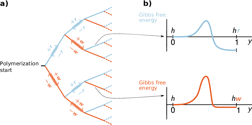
where $h$ is the heteropolymer produced so far, and $hr$ / $hw$ are the same heteropolymer with an addition of a $r$ / $w$ monomer at the tip, respectively. Each monomer incorporation is iteratively followed by a new one, so that the whole polymerization process is described by the tree-shaped network of chemical reactions Bennett 1979; Pigolotti and Sartori 2016 in Fig. 1a.

To achieve accurate and fast assembly, the reactions in Eq.(1) involve several intermediate steps, such as initial monomer discrimination Kunkel and Bebenek 2000, kinetic proofreading, Hopfield 1974; Ninio 1975; Kunkel and Bebenek 2000, and mismatch repair O’Donnell et al. 2013; Kunkel and Erie 2015. In general, each one of these error-correction mechanisms contribute simultaneously to polymerization accuracy, speed Rodnina and Wintermeyer 2001; Andrieux and Gaspard 2008; Johansson et al. 2008; Gaspard and Andrieux 2014; Banerjee et al. 2017; Sartori and Pigolotti 2015; Savir and Tlusty 2013; Sartori and Pigolotti 2013; Murugan et al. 2012, and energetic cost Cady and Qian 2009; Kramers 1940; Rao and Peliti 2015; Sartori and Pigolotti 2015; Wagoner and Dill 2019.

Refer to caption — Figure 1: Synthesis of heteropolymers. a) Network of incorporation and removal reactions to synthesize a heteropolymer. Each edge in the network represent the chemical reaction $h\rightleftharpoons hx$ where $h$ is the heteropolymer produced so far and $hx$ is the same heteropolymer with addition of monomer $x\in\{r,w\}$ at the tip. Three reactions compete at the nodes of the network: removal of the last incorporated monomer, incorporation of a $r$ monomer, and incorporation of a $w$ monomer. b) Reaction coordinate description of the incorporation and removal reactions. The initial and final points of the free energy landscapes correspond to the reactants and products of the incorporation and removal reactions, respectively.

Two approaches can provide insight into the error-correction mechanisms underlying heteropolymer assembly. The first approach is to measure their kinetic rates under different experimental conditions Rodnina and Wintermeyer 2001. The second approach is to simulate heteropolymer assembly using molecular dynamics Bock et al. 2018. From the molecular dynamics, one can project the numerous degrees of freedom into a 1-dimensional collective variable called reaction coordinate Banushkina and Krivov 2016. The reaction coordinate simplifies a chemical process into a one-dimensional random motion Banushkina and Krivov 2016; Socci et al. 1996; Best and Hummer 2006. The parameters of this random motion depend on the underlying reactants dynamics Zwanzig 1961; Berezhkovskii and Szabo 2013; Lu and Vanden-Eijnden 2014 and on the projection technique Lu and Vanden-Eijnden 2014; Banushkina and Krivov 2016; Krivov and Karplus 2006.

While successful in describing protein folding Socci et al. 1996; Best and Hummer 2006; Klimov and Thirumalai 1997 and in modeling reaction rates Kramers 1940; Klimov and Thirumalai 1997, approaches based on reaction coordinates found little use in studies of polymerization speed and accuracy. In principle, both reactions in Eq. (1) can be described by means of a reaction coordinate (Fig. 1b). However, to study the complete polymerization process we need to join the reaction coordinates characterizing each branch in Fig. 1a. Mathematically, this amounts to impose appropriate boundary conditions at the nodes of the reaction network.

In this paper, we develop a model of heteropolymer assembly based on reaction coordinates, and use it to compute the accuracy and speed of polymerization in different conditions. The paper is organized as follows. In Section II, we introduce our model. From the reaction coordinate, we derive effective incorporation and removal probabilities of right and wrong monomers. In Section III, we compute the accuracy and speed of a general heteropolymer assembly. In Section IV we consider examples characterized by different Gibbs free energy landscapes. In Section V, we generalize our results to a case where the reaction leading to monomer incorporation is complemented by kinetic proofreading. Section VI is devoted to conclusions and perspectives.

II Model

We define our model of heteropolymer assembly with reaction coordinates through the following steps. We first introduce the reaction coordinate and the free energy landscape in each chemical reaction of the polymerization network. We then study the dynamics of the reaction coordinate dynamics and its boundary conditions at the nodes of the network. Finally, we compute the probabilities to incorporate/remove one monomer along each reaction coordinate.

II.1 Reaction coordinate and Gibbs free energy of the heteropolymer

We introduce the continuous reaction coordinate $y$ along each edge of the polymerization network, Fig. 1a. Without loss of generality, we choose the units of the reaction coordinate so that $y\in[0,1]$ , where $y=0$ and $y=1$ correspond to $h$ and $hx$ respectively, i.e. to the states before and after monomer incorporation, see Figure 1.b.

Each point along this reaction coordinate is characterized by a Gibbs free energy $G^{hx}(y)$ (from now on simply ”free energy”). Such free energy depends on the previously incorporated sequence of monomers ( $h$ ), on the candidate monomer to be incorporated ( $x$ ) and on the stage of the incorporation process, i.e. the value of $y$ . Implicitly, $G^{hx}(y)$ also depends on the reactant and product concentrations.

We introduce the free energy increments from the beginning of each incorporation reaction

\Delta G^{x}(y)=G^{hx}(y)-G^{hx}(0),

(2)

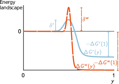
see Fig. 2. The free energy increments depend on the candidate monomer $x$ but not on the whole history of incorporated monomers $h$ . With this notation, the (absolute) binding free energy of monomer $x$ is equal to $-\Delta G^{x}(1)$ .

The free energy must be a continuous function of $y$ , and must also vary continuously when crossing the nodes of the network in Fig. 1. This means that we can decompose the free energy at an arbitrary stage of the polymerization process as

$\displaystyle G^{hx}(y)=$	$\displaystyle G^{hx}(0)+\Delta G^{x}(y)$	(3)
$\displaystyle=$	$\displaystyle G^{h}(1)+\Delta G^{x}(y)$
$\displaystyle=$	$\displaystyle\left(\sum_{i\in h}\Delta G^{i}(1)\right)+\Delta G^{x}(y).$

II.2 Stochastic dynamics of the reaction coordinate and boundary conditions

Because of thermal fluctuations, the reaction coordinate $y$ evolves according to a Langevin equation

\frac{\mathrm{d}y}{\mathrm{d}t}=-\mu\frac{\mathrm{d}}{\mathrm{d}y}G^{hx}(y)+\sqrt{2D}~\xi(t)

(4)

where $\mu$ is a mobility, $D$ is a diffusion coefficient, and $\xi(t)$ is white noise with $\langle\xi(t)\rangle=0$ and $\langle\xi(t)\xi(t^{\prime})\rangle=\delta(t-t^{\prime})$ Gardiner 2009. We assume that $D$ satisfies the Einstein relation $D=k_{B}T\mu$ with temperature $T$ and Boltzmann constant $k_{B}$ . We also assume that $D$ , $\mu$ , and $T$ are constant. When the reaction coordinate reaches the boundaries, either $y=0$ or $y=1$ , a new incorporation/removal reaction is commenced.

Equation (4) needs to be complemented by rules to specify which reaction initiates at the nodes of the reaction network. To this aim, we consider two intermediate values of the reaction coordinate: $y=\epsilon$ and $y=1-\epsilon$ with $\epsilon\ll 1$ . Using these values we coarse-grain the evolution of the reaction coordinate $y$ as

(y=0)\xrightleftharpoons[\pi_{\epsilon,0}^{x}]{\pi_{0,\epsilon}^{x}}(y=\epsilon)\xrightleftharpoons[\pi_{1-\epsilon,\epsilon}^{x}]{\pi_{\epsilon,1-\epsilon}^{x}}(y=1-\epsilon)\xrightleftharpoons[\pi_{1,1-\epsilon}^{x}]{\pi_{1-\epsilon,1}^{x}}(y=1)

(5)

where the quantities $\pi_{\tilde{y},y}^{x}$ are first-passage probability from $y$ to $\tilde{y}$ . For example, $\pi_{1-\epsilon,\epsilon}^{x}$ is the probability that the reaction coordinate reaches $y=1-\epsilon$ from $y=\epsilon$ without having reached $y=0$ before.

The representation in Eq.(5) separates the dynamics in proximity of the nodes of Fig. 1.b, from the dynamics in the interval $[\epsilon,1-\epsilon]$ . Thanks to this separation, we use detailed balance, probability conservation close to the nodes, and the continuity of $G^{hx}(y)$ to compute the first-passage probabilities $\pi_{\epsilon,0}^{x}$ and $\pi_{1-\epsilon,1}^{x}$ (see Appendix A). This procedure results in

\pi_{\epsilon,0}^{x}=\pi_{1-\epsilon,1}^{x}=\frac{1}{3}+\mathcal{O}(\epsilon).

(6)

We compute the first-passage probabilities in the interior applying standard techniques Gardiner 2009; Iyer-Biswas and Zilman 2016 to the Fokker-Planck equation associated to Eq. (4). We obtain

$\displaystyle\pi_{0,\epsilon}^{x}$	$\displaystyle=$	$\displaystyle\frac{\int_{\epsilon}^{1-\epsilon}\psi^{x}(y)\mathrm{d}y}{\int_{0}^{1-\epsilon}\psi^{x}(y)\mathrm{d}y}$
$\displaystyle\pi_{\epsilon,1-\epsilon}^{x}$	$\displaystyle=$	$\displaystyle\frac{\int_{1-\epsilon}^{1}\psi^{x}(y)\mathrm{d}y}{\int_{\epsilon}^{1}\psi^{x}(y)\mathrm{d}y}$
$\displaystyle\pi_{1-\epsilon,\epsilon}^{x}$	$\displaystyle=$	$\displaystyle\frac{\int_{0}^{\epsilon}\psi^{x}(y)\mathrm{d}y}{\int_{0}^{1-\epsilon}\psi^{x}(y)\mathrm{d}y}$
$\displaystyle\pi_{1,1-\epsilon}^{x}$	$\displaystyle=$	$\displaystyle\frac{\int_{\epsilon}^{1-\epsilon}\psi^{x}(y)\mathrm{d}y}{\int_{\epsilon}^{1}\psi^{x}(y)\mathrm{d}y}$	(7)

with

	$\displaystyle\psi^{x}(y)=$	$\displaystyle\exp\left[\int_{0}^{y}\frac{\mu}{D}\frac{\partial\Delta G^{x}(z)}{\partial z}\mathrm{d}z\right]$		(8)
	$\displaystyle=$	$\displaystyle\exp\left[\frac{\Delta G^{x}(y)}{k_{\mathrm{B}}T}\right]$		(8)

where the last equality follows from the relation $D=k_{B}T\mu$ .

II.3 Effective probabilities of monomer incorporation/rejection

From the probabilities $\pi_{\tilde{y},y}^{x}$ , we now compute the effective probabilities $p_{\rightarrow}^{x}$ and $p_{\leftarrow}^{x}$ to incorporate and reject monomer $x$ along each edge of the reaction network in Figure 1. To this end, we assume that the coarse grained dynamics in Eq.(5) is at steady state. We then use adiabatic elimination Pigolotti and Vulpiani 2008 to obtain (see Appendix B)


$\displaystyle p_{\rightarrow}^{x}=$	$\displaystyle{\frac{\epsilon}{3}}\,\frac{1}{\int_{0}^{1}\exp[\frac{\Delta G^{x}(y)}{k_{\mathrm{B}}T}]\,\mathrm{d}y}+\mathcal{O}(\epsilon)$	(9a)
$\displaystyle p_{\leftarrow}^{x}=$	$\displaystyle{\frac{\epsilon}{3}}\,\frac{e^{\frac{\Delta G^{x}(1)}{k_{\mathrm{B}}T}}}{\int_{0}^{1}\exp\left[\frac{\Delta G^{x}(y)}{k_{\mathrm{B}}T}\right]\,\mathrm{d}y}+\mathcal{O}(\epsilon)$	(9b)

Equations (9) relate the free energy landscapes $G^{x}(y)$ and the incorporation/removal probabilities of the polymerization process. They are consistent with the detailed balance condition

\frac{p^{x}_{\rightarrow}}{p_{\leftarrow}^{x}}=\exp\left[-\frac{\Delta G^{x}(1)}{k_{\mathrm{B}}T}\right].

(10)

which connects the ratios of forward and backward probabilities to the binding free energy $-\Delta G^{x}(1)$ , see Fig. 2.

III Results

We now address the accuracy and speed of a polymerization process in the reaction coordinate framework. We consider a copy polymer made up of a number $N^{r}$ of right monomers and $N^{w}$ of wrong monomers with $N=N^{r}+N^{w}$ . For large $N$ , we define the error rate

\eta=\lim_{N\rightarrow\infty}\frac{N^{w}}{N}.

(11)

To compute $\eta$ from the incorporation and removal probabilities $p_{\rightarrow}^{x}$ and $p_{\leftarrow}^{x}$ , we first recast Eq.(11) into the implicit equation

\frac{\eta}{1-\eta}=\lim_{N\rightarrow\infty}\frac{N^{w}}{N^{r}}=\lim_{n\rightarrow\infty}\frac{n^{w}_{\rightarrow}-n^{w}_{\leftarrow}}{n^{r}_{\rightarrow}-n^{r}_{\leftarrow}}

(12)

where we have introduced the numbers $n_{\rightarrow}^{r}$ , $n_{\leftarrow}^{r}$ , $n_{\rightarrow}^{w}$ and $n_{\leftarrow}^{w}$ of $r$ and $w$ incorporation and removal reactions which have occurred in the process, and $n$ is the total number of observed chemical reactions. For large $n$ we have


$\displaystyle n_{\rightarrow}^{r}\sim~$	$\displaystyle n\,c\,p_{\rightarrow}^{r}$	(13a)
$\displaystyle n_{\leftarrow}^{r}\sim~$	$\displaystyle n\,c\,(1-\eta)\,p_{\leftarrow}^{r}$	(13b)
$\displaystyle n_{\rightarrow}^{w}\sim~$	$\displaystyle n\,c\,p_{\rightarrow}^{w}$	(13c)
$\displaystyle n_{\leftarrow}^{w}\sim~$	$\displaystyle n\,c\,\eta\,p_{\leftarrow}^{w}$	(13d)

where $c=[p_{\rightarrow}^{r}+(1-\eta)p_{\leftarrow}^{r}+p_{\rightarrow}^{w}+\eta p_{\leftarrow}^{w}]^{-1}$ is a normalization constant so that $n=n_{\rightarrow}^{r}+n_{\leftarrow}^{r}+n_{\rightarrow}^{w}+n_{\leftarrow}^{w}=n$ . Substituting Eqs. (13) into Eq. (12) gives

\frac{\eta}{1-\eta}=\frac{p^{w}_{\rightarrow}-\eta p^{w}_{\leftarrow}}{p^{r}_{\rightarrow}-(1-\eta)p^{r}_{\leftarrow}}

(14)

Equation (14) is a general ”self-consistency” relation for the error rate that holds also for discrete models of polymerization Sartori and Pigolotti 2015; Pigolotti and Sartori 2016; Bennett 1979. In our case, we substitute Eqs. (9) in Eq. (14) and take the limit $\epsilon\to 0$ , obtaining

\displaystyle\frac{\eta}{1-\eta}=

\displaystyle\left(\frac{\eta-\exp\left[{-\frac{\Delta G^{w}(1)}{k_{\mathrm{B}}T}}\right]}{1-\eta-\exp\left[{-\frac{\Delta G^{r}(1)}{k_{\mathrm{B}}T}}\right]}\right)\ \left(\exp\left[{\tfrac{\Delta G^{w}(1)-\Delta G^{r}(1)}{k_{\mathrm{B}}T}}\right]\ \frac{\int_{0}^{1}\exp\left[\frac{\Delta G^{r}(y)}{k_{\mathrm{B}}T}\right]\,\mathrm{d}y}{\int_{0}^{1}\exp\left[\frac{\Delta G^{w}(y)}{k_{\mathrm{B}}T}\right]\,\mathrm{d}y}\right).

(15)

Solving Eq. 15 for $\eta$ yields an explicit expression of the error rate from the energy potentials.

Equation 15 identifies different regimes of error correction. To identify a first regime, we observe that

\eta=\frac{1}{1+\exp\left[\frac{\Delta G^{w}(1)-\Delta G^{r}(1)}{k_{\mathrm{B}}T}\right]}\quad\mbox{if }\quad\exp\left[{\tfrac{\Delta G^{w}(1)-\Delta G^{r}(1)}{k_{\mathrm{B}}T}}\right]\ \frac{\int_{0}^{1}\exp\left[\frac{\Delta G^{r}(y)}{k_{\mathrm{B}}T}\right]\,\mathrm{d}y}{\int_{0}^{1}\exp\left[\frac{\Delta G^{w}(y)}{k_{\mathrm{B}}T}\right]\,\mathrm{d}y}=1,

(16)

In the regime where Eq. (16) holds, the error depends only on the binding free energy difference $\Delta G^{w}(1)-\Delta G^{r}(1)$ . This regime is called energetic discrimination regime in the literature Sartori and Pigolotti 2013; Pigolotti and Sartori 2016. Systems near equilibrium operates in this regime because the Boltzmann factors of the binding free energies determine, via detailed balance, the probabilities to incorporate different monomers.

To identify a second error-correction regime in Eq. (15), we consider the case where $\Delta G^{r}(y)$ and $\Delta G^{w}(y)$ are characterized by energy barriers with heights $\delta^{r}$ and $\delta^{w}$ respectively (see Figure 1.b and Kramers Kramers 1940). When such barriers are large, we can approximate the integrals in Eq. (15) by using the Laplace method Bender and Orszag 1978

\frac{\int_{0}^{1}\exp\left[\frac{\Delta G^{r}(y)}{k_{\mathrm{B}}T}\right]\,\mathrm{d}y}{\int_{0}^{1}\exp\left[\frac{\Delta G^{w}(y)}{k_{\mathrm{B}}T}\right]\,\mathrm{d}y}\approx\exp\left[\frac{\delta^{r}-\delta^{w}}{k_{\mathrm{B}}T}\right]\sqrt{\frac{\Sigma^{w}}{\Sigma^{r}}}

(17)

where $\Sigma^{r}$ and $\Sigma^{w}$ are the curvatures of $\Delta G^{r}(y)$ and $\Delta G^{w}(y)$ at their maxima, respectively. Equation 17 implies that activation barriers suppress the polymerization error via the second term in round brackets in Eq. (15). The regime where this suppression occurs is the kinetic discrimination regime Sartori and Pigolotti 2013; Pigolotti and Sartori 2016. The first factor on the right-hand side of Eq. (17) represents the contribution of a difference in activation energy barrier $\delta^{r}-\delta^{w}$ to accuracy. This effect is also present in models based on discrete-step reactions Bennett 1979; Cady and Qian 2009; Sartori and Pigolotti 2013; Pigolotti and Sartori 2016. The factor $\sqrt{\Sigma^{w}/\Sigma^{r}}$ is a correction to activation energies based on the width of the activation barriers. This factor permits kinetic discrimination at equal barrier heights, provided that the barrier for right monomers is significantly more narrow than for wrong monomers.

We estimate the average polymerization speed using a similar argument to that leading to Eq. (15). For large number $N$ of incorporated monomers, the average speed is equal to $N$ divided the total time $\mathcal{T}$ needed to assemble the polymer

	$\displaystyle v=$	$\displaystyle\lim_{N\to\infty}\frac{N}{\mathcal{T}}$		(18)
	$\displaystyle=$	$\displaystyle\lim_{N\to\infty}\frac{\left(n_{\rightarrow}^{r}-n_{\leftarrow}^{r}\right)+\left(n_{\rightarrow}^{w}-n_{\leftarrow}^{w}\right)}{\mathcal{T}}$		(18)

where we expressed $N$ in terms of the number of incorporation/removal reactions. For large $N$ we can approximate the polymerization time as

\mathcal{T}\sim n\langle\tau\rangle

(19)

where $\langle\tau\rangle$ is the average time it takes to either incorporate or remove a monomer. Substituting Eqs. (13) and (19) into Eq. (18) gives the estimate for the polymerization speed

v=\frac{c[p_{\rightarrow}^{r}-(1-\eta)p_{\leftarrow}^{r}+p_{\rightarrow}^{w}-\eta p_{\leftarrow}^{w}]}{\langle\tau\rangle}.

(20)

The numerator of Eq. (18) is the probability of an incorporation minus the probability of a removal, while the denominator provides the timescale of these events. In practice, calculating $\langle\tau\rangle$ is not straightforward since one has to take into account contributions from incorporation attempts that are not finalized. In Appendix C, we provide a more formal derivation of Eq. (20), together with an explicit expression for $\langle\tau\rangle$ .

IV Examples

To address the validity and practical implications of Eqs. (15) and (20) we consider two examples of potentials $\Delta G^{r}(y)$ and $\Delta G^{w}(y)$ . In both cases, we work in dimensionless units by fixing $D=1$ , $k_{\mathrm{B}}T=1$ , and $\mu=1$ .

IV.1 Linear potential

As first example we consider linear free energy landscapes


	$\displaystyle\Delta G^{r}(y)=-m_{r}\,y$		(21a)
	$\displaystyle\Delta G^{w}(y)=-m_{w}\,y.$		(21b)

Despite their simplicity, the potentials in Eq. (21) are useful to understand the physics of the process. Upon increasing the slopes $m_{r}$ and $m_{w}$ , polymerization becomes increasingly irreversible. Substituting the potentials Eq. (21) into the expression for the error, Eq. (15) and performing the integrals we obtain

\frac{\eta}{1-\eta}=\frac{m_{w}(1-e^{-m_{r}})[1-e^{-m_{w}}\eta]}{m_{r}(1-e^{-m_{w}})[1+e^{-m_{r}}(1-\eta)]},

(22)

which implies

\eta=\frac{m_{w}}{m_{r}+m_{w}}\qquad\mbox{for}\qquad m_{r},m_{w}\gg 1.

(23)

The exact solution of Eq. (22) shows that the error is approximately a function of $m_{w}/m_{r}$ when $m_{r}$ , $m_{w}$ are large, as predicted by Eq. (23), Fig. 3a. We compared the predictions from Eqs. (22) and (20) with numerical simulations of the incorporation process from Eq.(4). Our theory yields reliable predictions for a broad range of parameters, Fig. 3c and 3d.

IV.2 Potential with an activation barrier

As a second example we consider the potential

\displaystyle\Delta G^{x}(y)=

\displaystyle a_{x}\left(e^{-\frac{\left(y-\frac{1}{2}\right)^{2}}{2c_{x}^{2}}}-e^{-\frac{1}{8c_{x}^{2}}}\right)+\frac{b_{x}}{2}\left(\frac{2c_{x}+\frac{1}{2}-y}{\sqrt{\left(2c_{x}+\frac{1}{2}-y\right)^{2}+c_{x}^{2}}}-\frac{2c_{x}+\frac{1}{2}}{\sqrt{\left(2c_{x}+\frac{1}{2}\right)^{2}+c_{x}^{2}}}\right)

(24)

where $a_{x}$ , $b_{x}$ and $c_{x}$ are monomer-dependent parameters that control the shape of the free energy potentials. Key features of the potential of Eq. (24) are the binding energy $-\Delta G^{x}(1)$ , the height of the activation barrier $\delta^{x}$ and its width $\sigma^{x}=4c_{x}$ , Fig. 4.

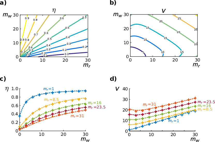
We study this model for different cases, corresponding to different parameter choices. In the first case we fix $-\Delta G^{r}(1)=-\Delta G^{w}(1)$ upon choosing $b_{r}=b_{w}=b$ and $c_{r}=c_{w}=1/20$ . This enforces a kinetic discrimination regime Pigolotti and Sartori 2016 where the binding energy $-\Delta G^{r}(1)$ quantifies the degree of irreversibility. For highly irreversible processes, the error $\eta$ should mainly depend on the activation energy difference $\delta^{r}-\delta^{r}$ , see Eq. (17). We also expect that the reaction speed should increase for more irreversible processes. Equations (15) and (20) confirm such qualitative picture, see Figure 5a and b. Also in this case, numerical simulations are in excellent quantitative agreement with our theory, Fig. 5c and 5d.

As a second case, we fix $a_{r}=a_{w}=5$ and $b_{r}=b_{w}=1$ . In this way we have that $-\Delta G^{r}(1)\approx-\Delta G^{w}(1)$ and $\delta^{r}\approx\delta^{w}$ . Energetics alone would not permit monomer discrimination in this case Pigolotti and Sartori 2016. However, Eq. (17) predicts that the difference in the barrier widths $\sigma_{r}$ and $\sigma_{w}$ should allow to discriminate $r$ and $w$ monomers (see Figure 6.a). We confirmed the existence of such kinetic discrimination regime with numerical simulations, Fig. 6.c.

V Kinetic proofreading

In this Section we sketch a generalization of our framework to include kinetic proofreading Hopfield 1974; Ninio 1975. We assume that the reaction $h\rightleftharpoons hx$ can be decomposed into three sub-reactions

(25)

where each sub-reaction occurs with probabilities $p_{\rightarrow}^{i,x}$ s and $p_{\leftarrow}^{i,x}$ s, and $hx^{*}$ is an intermediate meta-stable complex. The extra pathway $hx^{*}\rightleftharpoons h$ represents kinetic proofreading. Such reaction can improve accuracy when driven towards the reactants $h$ , so that wrong monomers undergo an additional checkpoint. Hopfield 1974; Pigolotti and Sartori 2016.

Every sub-reactions in Eq. (25) is described by its own reaction coordinate $y$ which evolves according to a Langevin equation

\frac{\mathrm{d}y}{\mathrm{d}t}=-\mu\frac{\mathrm{d}}{\mathrm{d}y}G^{i,x}(y)+\sqrt{2D}~\xi(t)

(26)

where $G^{i,hx}(y)$ is the free energy landscapes along the $i$ -th sub-reaction. Also in this case we take $y\in[0,1]$ for all sub-reactions, with $y=1$ always in the direction of incorporation of monomer $x$ . Similarly to Eq. (3), we decompose the free energies for the sub-reactions as


$\displaystyle G^{1,h\tilde{x}x}(y)=$	$\displaystyle\Delta G^{1,x}(y)+G^{2,h\tilde{x}}(1)$	(27a)
$\displaystyle G^{2,h\tilde{x}x}(y)=$	$\displaystyle\Delta G^{2,x}(y)+G^{1,h\tilde{x}x}(1)$	(27b)
$\displaystyle G^{3,h\tilde{x}x}(y)=$	$\displaystyle\begin{cases}\Delta G^{3,x}(y)+G^{2,h\tilde{x}}(1)\quad\mbox{for }hx^{}\rightarrow h\\ \Delta G^{3,x}(y)+G^{1,h\tilde{x}x}(1)\quad\mbox{for }hx^{}\leftarrow h\end{cases}$	(27c)

where we specified that monomer $\tilde{x}$ was incorporated before attempting to incorporate monomer $x$ . Here, $G^{3,h\tilde{x}x}(y)$ depend on the direction of the sub-reaction because the heteropolymer total energy now depends also on the sequence of sub-reactions.

We now compute the probabilities $p_{\rightarrow}^{i,x}$ s and $p_{\leftarrow}^{i,x}$ with $i\in\{1,2,3\}$ from Eq. (26) with the same procedure which leads to Eq.(9). This yields


$\displaystyle p_{\rightarrow}^{i,x}=$	$\displaystyle\epsilon\,\pi_{\epsilon,0}^{i,x}\,\frac{1}{\int_{0}^{1}\exp[\frac{\Delta G^{i,x}(y)}{k_{\mathrm{B}}T}]\,\mathrm{d}y}+\mathcal{O}(\epsilon)$	(28a)
$\displaystyle p_{\leftarrow}^{i,x}=$	$\displaystyle\epsilon\,\pi_{1-\epsilon,1}^{i,x}\,\frac{e^{\frac{\Delta G^{i,x}(1)}{k_{\mathrm{B}}T}}}{\int_{0}^{1}\exp[\frac{\Delta G^{i,x}(y)}{k_{\mathrm{B}}T}]\,\mathrm{d}y}+\mathcal{O}(\epsilon).$	(28b)

with


$\displaystyle\pi_{\epsilon,0}^{1,x}=\pi_{1-\epsilon,1}^{2,x}=\pi_{\epsilon,0}^{3,x}$	$\displaystyle=\frac{1}{5}$	(29a)
$\displaystyle p_{1-\epsilon,1}^{1,x}=\pi_{\epsilon,0}^{2,x}=\pi_{\epsilon,0}^{3,x}$	$\displaystyle=\frac{1}{3}.$	(29b)

Equations (29) state that the all sub-reactions from reactants $h$ and $hx^{*}$ respectively can start with equal probabilities.

To obtain an equation for $\eta$ , we need to compute the effective incorporation and removal probabilities $p_{\rightarrow}^{x}$ and $p_{\leftarrow}^{x}$ in Eq. (14) from Eqs. (28) and (29). To this end we assume that the reactions in Eq.(25) are at steady state. We then use adiabatic elimination Pigolotti and Vulpiani 2008 to obtain (see Appendix D)


$\displaystyle p_{\rightarrow}^{x}=$	$\displaystyle\frac{p_{\rightarrow}^{2,x}(p_{\rightarrow}^{1,x}+p_{\rightarrow}^{3,x})}{p_{\leftarrow}^{1,x}+p_{\leftarrow}^{3,x}+p_{\rightarrow}^{2,x}}$	(30a)
$\displaystyle p_{\leftarrow}^{x}=$	$\displaystyle\frac{p_{\leftarrow}^{2,x}(p_{\leftarrow}^{1,x}+p_{\leftarrow}^{3,x})}{p_{\leftarrow}^{1,x}+p_{\leftarrow}^{3,x}+p_{\rightarrow}^{2,x}}$	(30b)

Substituting Eqs. (28) and (30) in Eq. (14) finally provides an expression for $\eta$ in terms of the free energy landscapes $G^{i,x}(y)$ .

VI Conclusions

In this paper, we described assembly of heteropolymers by means of continuous reaction coordinates. In the simplest cases, our results are consistent with those derived for reactions occurring in discrete steps Andrieux and Gaspard 2008; Gaspard and Andrieux 2014; Banerjee et al. 2017; Sartori and Pigolotti 2015; Sartori and Pigolotti 2013; Murugan et al. 2012; Pigolotti and Sartori 2016; Bennett 1979. Moreover, our formalism reveals discrimination mechanisms that are not easily described with discrete reactions. One example is the possibility to discriminate according to barrier widths, as described by Eq. (17) and confirmed in simulations, Fig. 6c.

For simplicity, in this paper we developed our formalism by means of a reaction coordinate characterized by a Markovian dynamic. In general, only specific projection techniques yield reaction coordinates with negligible non-Markovian contributions Banushkina and Krivov 2016; Lu and Vanden-Eijnden 2014; Krivov and Karplus 2006; Krivov 2018, and the resulting Langevin equation might not be in the form of Eq. (4). Our framework can be adapted to such situations as well as to non-Markovian reaction coordinates, describing for example enzymes undergoing slow conformational changes.

The framework described here is microscopically reversible. This allows to characterize non-equilibrium work and heat exchanges during the polymerization process from the diffusive dynamics of the reaction coordinate, similarly to recent studies of the ATP synthase Lucero et al. 2019; Kasper and Sivak 2019 and small-scale technological devices Neri et al. 2015; López-Suárez et al. 2016. This analysis would permit to characterize thermodynamic limits of information processing of these processes Bérut et al. 2012; Jun et al. 2014; Chiuchiú 2015; Sartori and Pigolotti 2015.

Acknowledgements.

This work was supported by JSPS KAKENHI Grant Number JP18K03473 (to DC and SP).

Appendix A First passage time probabilities at the nodes

Because of detailed balance, the probabilities $\pi_{\epsilon,0}^{x}$ and $\pi_{1-\epsilon,1}^{x}$ are related to the free energy difference when passing from one edge of the reaction network to another, i.e.

	$\displaystyle\pi_{\epsilon,0}^{x}$	$\displaystyle\propto$	$\displaystyle\exp\left[-\frac{G^{h\tilde{x}x}(\epsilon)}{k_{\mathrm{B}}T}\right]$
	$\displaystyle\pi_{1-\epsilon,1}^{\tilde{x}}$	$\displaystyle\propto$	$\displaystyle\exp\left[-\frac{G^{h\tilde{x}}(1-\epsilon)}{k_{\mathrm{B}}T}\right].$		(31)

where we specified that the monomer $\tilde{x}\in\{r,w\}$ was incorporated before monomer $x\in\{r,w\}$ . After the incorporation of $\tilde{x}$ , the enzyme can catalyze three reactions: removal of $\tilde{x}$ or incorporation of either $r$ or $w$ . The probabilities of these three events must be normalized

\pi_{1-\epsilon,1}^{\tilde{x}}+\pi_{\epsilon,0}^{r}+\pi_{\epsilon,0}^{w}=1.

(32)

Combining Eqs.(A)-(32) gives


$\displaystyle\pi_{\epsilon,0}^{x}=$	$\displaystyle\frac{\exp\left[-\frac{G^{h\tilde{x}x}(\epsilon)-G^{h\tilde{x}}(1-\epsilon)}{k_{\mathrm{B}}T}\right]}{1+\exp\left[-\frac{G^{h\tilde{x}r}(\epsilon)-G^{h\tilde{x}}(1-\epsilon)}{k_{\mathrm{B}}T}\right]+\exp\left[-\frac{G^{h\tilde{x}w}(\epsilon)-G^{h\tilde{x}}(1-\epsilon)}{k_{\mathrm{B}}T}\right]}$	(33a)
$\displaystyle\pi_{1-\epsilon,1}^{\tilde{x}}=$	$\displaystyle\frac{1}{1+\exp\left[-\frac{G^{h\tilde{x}r}(\epsilon)-G^{\tilde{x}}(1-\epsilon)}{k_{\mathrm{B}}T}\right]+\exp\left[-\frac{G^{h\tilde{x}w}(\epsilon)-G^{h\tilde{x}}(1-\epsilon)}{k_{\mathrm{B}}T}\right]}.$	(33b)

Substituting Eq.(3) into Eq.(33), taking the limit of small $\epsilon$ , using the continuity of $G^{h\tilde{x}x}(y)$ and then renaming $\tilde{x}$ with $x$ finally gives Eq.(6).

Appendix B Effective incorporation and removal probabilities

The dynamics of the reaction coordinate $y$ in the coarse grained description of Eq.(5) obeys a Markov chain


$\displaystyle P_{0}^{x}(\nu+1)=$	$\displaystyle\pi_{0,\epsilon}^{x}P_{\epsilon}^{x}(\nu)+\left[1-\pi_{\epsilon,0}^{x}\right]P_{0}^{x}(\nu)+\mbox{external fluxes }$	(34a)
$\displaystyle\begin{split}P_{\epsilon}^{x}(\nu+1)=&\pi_{\epsilon,0}^{x}P_{0}^{x}(\nu)+\pi_{\epsilon,1-\epsilon}^{x}P_{1-\epsilon}^{x}(\nu)+\left[1-\left(\pi_{0,\epsilon}^{x}+\pi_{1-\epsilon,\epsilon}^{x}\right)\right]P_{\epsilon}^{x}(\nu)\end{split}$		(34b)
$\displaystyle\begin{split}P_{1-\epsilon}^{x}(\nu+1)=&\pi_{1-\epsilon,\epsilon}^{x}P_{\epsilon}^{x}(\nu)+\pi_{1-\epsilon,1}^{x}P_{1}^{x}(\nu)+\left[1-\left(\pi_{\epsilon,1-\epsilon}^{x}+\pi_{1,1-\epsilon}^{x}\right)\right]P_{1-\epsilon}^{x}(\nu)\end{split}$		(34c)
$\displaystyle P_{1}^{x}(\nu+1)=$	$\displaystyle\pi_{1,1-\epsilon}^{x}P_{1-\epsilon}^{x}(\nu)+\left[1-\pi_{1-\epsilon,1}^{x}\right]P_{1}^{x}(\nu)+\mbox{external fluxes}.$	(34d)

where the first-passage probabilities appear as transition probabilities, and the quantities $P^{x}_{0}(\nu)$ , $P_{\epsilon}(\nu)$ , $P_{1-\epsilon}(\nu)$ , and $P_{1}(\nu)$ are the probabilities that the reaction coordinate reaches the point $y=0$ , $y=\epsilon$ , $y=1-\epsilon$ and $y=1$ after $\nu$ consecutive transitions respectively. The external fluxes in Eqs. (34a) and (34d) are the probability fluxes from the remaining reactions which originate from the nodes $y=0$ and $y=1$ in the network of Figure 1.a.

To simplify Eq. (34) we perform adiabatic elimination Pigolotti and Vulpiani 2008 of the intermediate states $y=\epsilon$ and $y=1-\epsilon$ : we impose the steady state regime $P_{\epsilon}^{x}(\nu+1)=P_{\epsilon}^{x}(\nu)$ and $P_{\epsilon}^{x}(\nu+1)=P_{\epsilon}^{x}(\nu)$ in Eqs.(34b) and (34c) respectively, we solve Eqs.(34b)-(34c) for $P_{\epsilon}^{x}(\nu)$ and $P_{1-\epsilon}^{x}(\nu)$ , and we finally substitute the result back into Eqs.(34a), (34d). This yield the effective Markov chain


$\displaystyle P_{0}^{x}(\nu+1)=$	$\displaystyle p_{\leftarrow}^{x}P_{1}^{x}(\nu)+\left[1-p_{\rightarrow}^{x}\right]P_{0}^{x}(\nu)+\mbox{external fluxes}$	(35a)
$\displaystyle P_{1}^{x}(\nu+1)=$	$\displaystyle p_{\rightarrow}^{x}P_{0}^{x}(\nu)+\left[1-p_{\leftarrow}^{x}\right]P_{1}^{x}(\nu)+\mbox{external fluxes }.$	(35b)

where we have defined the effective probabilities $p_{\rightarrow}^{x}$ and $p_{\leftarrow}^{x}$ to incorporate a monomer ( $h\rightarrow hx$ ) and remove a monomer ( $h\leftarrow hx$ ) respectively as


$\displaystyle p_{\rightarrow}^{x}=$	$\displaystyle\frac{\pi_{1,1-\epsilon}^{x}\pi_{1-\epsilon,\epsilon}^{x}\pi_{\epsilon,0}^{x}}{\pi_{1,1-\epsilon}^{x}\ \pi_{1-\epsilon,\epsilon}^{x}+\pi_{0,\epsilon}^{x}\ \pi_{\epsilon,1-\epsilon}^{x}+\pi_{0,\epsilon}^{x}\ \pi_{1,1-\epsilon}^{x}}$	(36a)
$\displaystyle p_{\leftarrow}^{x}=$	$\displaystyle\frac{\pi_{0,\epsilon}^{x}\ \pi_{\epsilon,1-\epsilon}^{x}\ \pi_{1-\epsilon,1}^{x}}{\pi_{1,1-\epsilon}^{x}\ \pi_{1-\epsilon,\epsilon}^{x}+\pi_{0,\epsilon}^{x}\ \pi_{\epsilon,1-\epsilon}^{x}+\pi_{0,\epsilon}^{x}\ \pi_{1,1-\epsilon}^{x}}.$	(36b)

Substituting Eq.(6)-(8) into Eq. (36) and then expanding for small $\epsilon$ finally gives Eq. (9).

Appendix C Derivation of the polymerization speed via reaction coordinates.

To derive the polymerization speed, we consider a mean field formulation of the polymerization process in Figure 1.a where the enzyme can remove any monomer in the copy heteropolymer. Removal of $r$ and $w$ monomers occurs with probabilities $1-\eta$ and $\eta$ respectively. This assumption simplifies the reaction tree of Figure 1.a into the closed network of Fig. 7.a, where the incorporation and removal probabilities $p_{\rightarrow}^{x}$ and $p_{\leftarrow}^{x}$ are defined as in Eq. (9).

We now introduce the reaction coordinate in this mean field description, Fig. 7.b. For later convenience, we also consider the values of the reaction coordinate $y=0$ $y=\epsilon$ , $y=1-\epsilon$ and $y=1$ together with the probabilities $\pi_{\tilde{y},y}^{x}$ s defined in Eqs.(6) and (II.2).

Using the scheme in Figure 7.b, we define the probability $P_{0,1}(\zeta)$ that $y=0$ or $y=1$ after $\zeta$ consecutive transitions, and the probabilities $P_{\epsilon}^{r}(\zeta)$ , $P_{1-\epsilon}^{r}(\zeta)$ , $P_{\epsilon}^{w}(\zeta)$ , $P_{1-\epsilon}^{w}(\zeta)$ that $y=\epsilon$ or $y=1-\epsilon$ for the $r$ and $w$ monomer after $\zeta$ consecutive transitions. These probabilities evolves according to the Markov chain

\vec{P}(\zeta+1)=\mathtt{A}\,\vec{P}(\zeta)

(37)

where

\vec{P}(\zeta)=\left(P_{0,1}(\zeta),P_{\epsilon}^{r}(\zeta),P_{1-\epsilon}^{r}(\zeta),P_{\epsilon}^{w}(\zeta),P_{1-\epsilon}^{w}(\zeta)\right)^{\mathtt{T}}

(38)

and

\mathtt{A}=\begin{bmatrix}0&\pi_{0,\epsilon}^{r}&\pi_{1,1-\epsilon}^{r}&\pi_{0,\epsilon}^{w}&\pi_{1,1-\epsilon}^{w}\\ c^{\prime}\,\pi_{\epsilon,0}^{r}&0&\pi_{\epsilon,1-\epsilon}^{r}&0&0\\ c^{\prime}\,(1-\eta)\pi_{1-\epsilon,1}^{r}&\pi_{1-\epsilon,\epsilon}^{r}&0&0&0\\ c^{\prime}\,\pi_{\epsilon,0}^{w}&0&0&0&\pi_{\epsilon,1-\epsilon}^{w}\\ c^{\prime}\,\eta\pi_{1-\epsilon,1}^{w}&0&0&\pi_{1-\epsilon,\epsilon}^{w}&0\end{bmatrix}

(39)

where $c^{\prime}=[\pi_{\epsilon,0}^{r}+(1-\eta)\pi_{1-\epsilon,1}^{r}+\pi_{\epsilon,0}^{w}+\eta\pi_{1-\epsilon,1}^{w}]$ is a normalization constant. We now define the matrices


$\displaystyle\mathtt{J}^{N}$	$\displaystyle=\frac{1}{3}\begin{bmatrix}0&-1&+1&-1&+1\\ +1&0&-1&0&0\\ -1&+1&0&0&0\\ +1&0&0&0&-1\\ -1&0&0&+1&0\end{bmatrix}$	(40a)
$\displaystyle\mathtt{J}^{\mathcal{T}}$	$\displaystyle=\begin{bmatrix}0&\langle\mathrm{d}\tau\rangle_{0,\epsilon}^{r}&\langle\mathrm{d}\tau\rangle_{1,1-\epsilon}^{r}&\langle\mathrm{d}\tau\rangle_{0,\epsilon}^{w}&\langle\mathrm{d}\tau\rangle_{1,1-\epsilon}^{w}\\ \langle\mathrm{d}\tau\rangle_{\epsilon,0}^{r}&0&\langle\mathrm{d}\tau\rangle_{\epsilon,1-\epsilon}^{r}&0&0\\ \langle\mathrm{d}\tau\rangle_{1-\epsilon,1}^{r}&\langle\mathrm{d}\tau\rangle_{1-\epsilon,\epsilon}^{r}&0&0&0\\ \langle\mathrm{d}\tau\rangle_{\epsilon,0}^{w}&0&0&0&\langle\mathrm{d}\tau\rangle_{\epsilon,1-\epsilon}^{w}\\ \langle\mathrm{d}\tau\rangle_{1-\epsilon,1}^{w}&0&0&\langle\mathrm{d}\tau\rangle_{1-\epsilon,\epsilon}&0\end{bmatrix}$	(40b)

which contain the contribution of each transition to the heteropolymer length $N$ and the polymerization time $\mathcal{T}$ . The time increments $\langle\mathrm{d}\tau\rangle_{y,\tilde{y}}^{x}$ in $\mathtt{J}^{\mathcal{T}}$ are the first passage times from $\tilde{y}$ to $y$ Gardiner 2009. In particular we have that


$\displaystyle\langle\tau\rangle_{0,\epsilon}^{x}=$	$\displaystyle\frac{1}{D}\ \left(\Phi_{\rightarrow}^{x}(0)-\frac{\int_{0}^{1}\Phi_{\rightarrow}^{x}(y)\mathrm{d}y}{\int_{0}^{1}\psi^{x}(y)\mathrm{d}y}\right)\epsilon+\mathcal{O}\left(\epsilon^{2}\right)$	(41a)
$\displaystyle\langle\tau\rangle_{1-\epsilon,\epsilon}=$	$\displaystyle\frac{1}{D}\ \int_{0}^{1}\Phi_{\leftarrow}^{x}(y)\mathrm{d}y+\mathcal{O}\left(\epsilon\right)$	(41b)
$\displaystyle\langle\tau\rangle_{\epsilon,1-\epsilon}=$	$\displaystyle\frac{1}{D}\ \int_{0}^{1}\Phi_{\rightarrow}^{x}(y)\mathrm{d}y+\mathcal{O}\left(\epsilon\right)$	(41c)
$\displaystyle\langle\tau\rangle_{1,1-\epsilon}^{x}=$	$\displaystyle\frac{1}{D}\ \left(\Phi_{\leftarrow}^{x}(1)-\left(e^{\frac{\Delta G^{x}(1)}{k_{\mathrm{B}}T}}\right)\frac{\int_{0}^{1}\Phi_{\leftarrow}^{x}(y)\mathrm{d}y}{\int_{0}^{1}\psi^{x}(y)\mathrm{d}y}\right)\epsilon+\mathcal{O}\left(\epsilon^{2}\right)$	(41d)

with


$\displaystyle\Phi_{\rightarrow}^{x}(y)$	$\displaystyle=\frac{\psi^{x}(y)\int_{y}^{1}\int_{u}^{1}\frac{\psi^{x}(z)}{\psi^{x}(u)}\mathrm{d}z\mathrm{d}u}{\int_{0}^{1}\psi^{x}(y)\mathrm{d}y}$	(42a)
$\displaystyle\Phi_{\leftarrow}^{x}(y)$	$\displaystyle=\frac{\psi^{x}(y)\int_{0}^{y}\int_{0}^{u}\frac{\psi^{x}(z)}{\psi^{x}(u)}\mathrm{d}z\mathrm{d}u}{\int_{0}^{1}\psi^{x}(y)\mathrm{d}y}.$	(42b)

The remaining first passage times $\langle\mathrm{d}\tau\rangle_{\epsilon,0}^{r}$ , $\langle\mathrm{d}\tau\rangle_{1-\epsilon,1}^{r}$ , $\langle\mathrm{d}\tau\rangle_{\epsilon,0}^{w}$ and $\langle\mathrm{d}\tau\rangle_{1-\epsilon,1}^{w}$ , are assumed equal to zero for simplicity. Physically, this assumption is justified when binding and unbinding of monomers is much faster than processing a monomer into a finalized incorporation.

Using Eq.(40) we define the tilted matrix $\mathtt{B}$ with components

\mathtt{B}_{i,j}=\mathtt{A}_{i,j}\exp\left[q_{N}\mathtt{J}^{N}_{i,j}+q_{\tau}\mathtt{J}^{\tau}_{i,j}\right]

(43)

and dummy variables $q_{N}$ , and $q_{\tau}$ . For large values of $\zeta$ , the largest eigenvalue of $\mathtt{B}$ coincides with the scaled cumulant generating function of $N$ and $\mathcal{T}$ , see Touchette 2009. The implicit function theorem then implies


	$\displaystyle N\approx-\zeta\left.\frac{\partial_{q_{N}}\det\left[\mathtt{B}-\lambda\mathtt{I}\right]}{\partial_{\lambda}\det\left[\mathtt{B}-\lambda\mathtt{I}\right]}\right\|_{q_{N}=q_{\tau}=0,\lambda=1}$		(44a)
	$\displaystyle\mathcal{T}\approx-\zeta\left.\frac{\partial_{q_{\tau}}\det\left[\mathtt{B}-\lambda\mathtt{I}\right]}{\partial_{\lambda}\det\left[\mathtt{B}-\lambda\mathtt{I}\right]}\right\|_{q_{N}=q_{\tau}=0,\lambda=1}$		(44b)

where $\det\left[\mathtt{B}-\lambda\mathtt{I}\right]$ is the characteristic polynomial of $\mathtt{B}$ . To compute $v$ we finally use that

v=\frac{N}{\mathcal{T}}=\left.\frac{\partial_{q_{N}}\det\left[\mathtt{B}-\lambda\mathtt{I}\right]}{\partial_{q_{\tau}}\det\left[\mathtt{B}-\lambda\mathtt{I}\right]}\right|_{q_{N}=q_{\tau}=0,\lambda=1}.

(45)

which is equivalent to Eq.(18). Substituting Eqs.(6), (II.2), (39), (40) and (43) into Eqs.(45) and then taking the leading order for small $\epsilon$ yields Eq. (20), where

	$\displaystyle\frac{\langle\tau\rangle D}{c}=$	$\displaystyle\left(p_{\rightarrow}^{r}-(1-\eta)p_{\leftarrow}^{r}\right)\left(\int_{0}^{1}\left[\Phi_{\leftarrow}^{r}(y)-\Phi_{\rightarrow}^{r}(y)\right]\mathrm{d}y\right)+\left(p_{\rightarrow}^{w}-\eta p_{\leftarrow}^{w}\right)\left(\int_{0}^{1}\left[\Phi_{\leftarrow}^{w}(y)-\Phi_{\rightarrow}^{w}(y)\right]\mathrm{d}y\right)$		(46)
		$\displaystyle{\displaystyle+\frac{\epsilon}{3}\,\Bigg(\Phi_{\rightarrow}^{r}(0)+\Phi_{\rightarrow}^{w}(0)+(1-\eta)\Phi^{r}_{\leftarrow}(1)+\eta\Phi^{w}_{\leftarrow}(1)\Bigg)+\mathcal{O}\left(\epsilon^{2}\right)}$		(46)

and $c$ is defined as in Eq. (13).

Appendix D Effetive incorporation and removal probabilities for the Kinetic proofreading example

To compute the incorporation and removal probabilities for the Kinetic proofreading case we mimic the procedure that leads to Eq.(9). We consider the probabilities $P_{h}(\xi)$ , $P_{hx^{*}}(\xi)$ and $P_{hx}(\xi)$ to obtain the reactants $h$ , $hx^{*}$ , and $hx$ after $\xi$ sub-reactions of Eq. (25). These probabilities evolve according to the Markov chain


$\displaystyle P_{h}(\xi+1)$	$\displaystyle=p_{\leftarrow}^{1,x}P_{hx^{x}}(\xi)+\left[1-\left(p_{\rightarrow}^{1,x}+p_{\rightarrow}^{3,x}\right)\right]P_{h}(\xi)+\mbox{external fluxes}$	(47a)
$\displaystyle P_{hx^{*}}(\xi+1)$	$\displaystyle=p_{\rightarrow}^{1,x}P_{h}(\xi)+p_{\leftarrow}^{2,x}P_{hx}(\xi)+p_{\rightarrow}^{3,x}P_{h}(\xi)+\left[1-\left(p_{\leftarrow}^{1,x}+p_{\rightarrow}^{2,x}+p_{\leftarrow}^{3,x}\right)\right]P_{hx^{*}}(\xi)$	(47b)
$\displaystyle P_{hx}(\xi+1)$	$\displaystyle=p_{\rightarrow}^{2,x}P_{hx^{*}}(\xi)+\left[1-p_{\leftarrow}^{2,x}\right]P_{hx}(\xi)+\mbox{external fluxes},$	(47c)

where the external fluxes are the probability fluxes of the other sub-reactions entering the nodes $y=0$ and $y=1$ . At steady state, we simplify Eq. (47) with adiabatic eliminationPigolotti and Vulpiani 2008: we impose $P_{hx^{*}}(\xi+1)=P_{hx^{*}}(\xi)$ into Eq. (47b), solve it for $P_{hx^{*}}(\xi)$ and substitute the solution in Eqs. (47a) and (47c). This yields, after some rearrangements,


$\displaystyle P_{h+x}(\xi+1)$	$\displaystyle=p_{\leftarrow}^{x}P_{hx}(\xi)+\left[1-p_{\rightarrow}^{x}\right]P_{h+x}(\xi)$	(48a)
$\displaystyle P_{hx}(\xi+1)$	$\displaystyle=p_{\rightarrow}^{x}P_{h+x}(\xi)+\left[1-p_{\leftarrow}^{x}\right]P_{hx}(\xi)$	(48b)

with effective incorporation/removal probabilities $p_{\rightarrow}^{x}$ and $p_{\leftarrow}^{x}$ defined as in Eq.(30).

References

Reynolds et al. (2010) N. M. Reynolds, B. A. Lazazzera, and M. Ibba, Nature Reviews Microbiology 8, 849 (2010).
Bennett (1979) C. H. Bennett, BioSystems 11, 85 (1979).
Pigolotti and Sartori (2016) S. Pigolotti and P. Sartori, Journal of Statistical Physics 162, 1167 (2016).
Kunkel and Bebenek (2000) T. A. Kunkel and K. Bebenek, Annual Review of Biochemistry 69, 497 (2000), pMID: 10966467.
Hopfield (1974) J. J. Hopfield, Proceedings of the National Academy of Sciences 71, 4135 (1974).
Ninio (1975) J. Ninio, Biochimie 57, 587 (1975).
O’Donnell et al. (2013) M. O’Donnell, L. Langston, and B. Stillman, Cold Spring Harbor Perspectives in Biology 5 (2013), 10.1101/cshperspect.a010108.
Kunkel and Erie (2015) T. A. Kunkel and D. A. Erie, Annual Review of Genetics 49, 291 (2015), pMID: 26436461.
Rodnina and Wintermeyer (2001) M. V. Rodnina and W. Wintermeyer, Annual Review of Biochemistry 70, 415 (2001), pMID: 11395413.
Andrieux and Gaspard (2008) D. Andrieux and P. Gaspard, Proceedings of the National Academy of Sciences 105, 9516 (2008).
Johansson et al. (2008) M. Johansson, M. Lovmar, and M. Ehrenberg, Current Opinion in Microbiology 11, 141 (2008), cell Regulation.
Gaspard and Andrieux (2014) P. Gaspard and D. Andrieux, The Journal of Chemical Physics 141, 044908 (2014).
Banerjee et al. (2017) K. Banerjee, A. B. Kolomeisky, and O. A. Igoshin, Proceedings of the National Academy of Sciences 114, 5183 (2017).
Sartori and Pigolotti (2015) P. Sartori and S. Pigolotti, Phys. Rev. X 5, 041039 (2015).
Savir and Tlusty (2013) Y. Savir and T. Tlusty, Cell 153, 471 (2013).
Sartori and Pigolotti (2013) P. Sartori and S. Pigolotti, Phys. Rev. Lett. 110, 188101 (2013).
Murugan et al. (2012) A. Murugan, D. A. Huse, and S. Leibler, Proceedings of the National Academy of Sciences 109, 12034 (2012).
Cady and Qian (2009) F. Cady and H. Qian, Physical biology 6, 036011 (2009).
Kramers (1940) H. Kramers, Physica 7, 284 (1940).
Rao and Peliti (2015) R. Rao and L. Peliti, Journal of Statistical Mechanics: Theory and Experiment 2015, P06001 (2015).
Wagoner and Dill (2019) J. A. Wagoner and K. A. Dill, Proceedings of the National Academy of Sciences 116, 5902 (2019), https://www.pnas.org/content/116/13/5902.full.pdf .
Bock et al. (2018) L. V. Bock, M. H. Kolář, and H. Grubmüller, Current Opinion in Structural Biology 49, 27 (2018).
Banushkina and Krivov (2016) P. V. Banushkina and S. V. Krivov, Wiley Interdisciplinary Reviews: Computational Molecular Science 6, 748 (2016), https://onlinelibrary.wiley.com/doi/pdf/10.1002/wcms.1276 .
Socci et al. (1996) N. D. Socci, J. N. Onuchic, and P. G. Wolynes, The Journal of Chemical Physics 104, 5860 (1996).
Best and Hummer (2006) R. B. Best and G. Hummer, Phys. Rev. Lett. 96, 228104 (2006).
Zwanzig (1961) R. Zwanzig, Phys. Rev. 124, 983 (1961).
Berezhkovskii and Szabo (2013) A. M. Berezhkovskii and A. Szabo, The Journal of Physical Chemistry B 117, 13115 (2013).
Lu and Vanden-Eijnden (2014) J. Lu and E. Vanden-Eijnden, The Journal of Chemical Physics 141, 044109 (2014).
Krivov and Karplus (2006) S. V. Krivov and M. Karplus, The Journal of Physical Chemistry B 110, 12689 (2006), pMID: 16800603.
Klimov and Thirumalai (1997) D. K. Klimov and D. Thirumalai, Phys. Rev. Lett. 79, 317 (1997).
Gardiner (2009) C. Gardiner, Stochastic Methods: A Handbook for the Natural and Social Sciences, Springer Series in Synergetics (Springer Berlin Heidelberg, 2009).
Iyer-Biswas and Zilman (2016) S. Iyer-Biswas and A. Zilman, “First-passage processes in cellular biology,” in Advances in Chemical Physics (John Wiley and Sons, Ltd, 2016) Chap. NONE, pp. 261–306.
Pigolotti and Vulpiani (2008) S. Pigolotti and A. Vulpiani, The Journal of Chemical Physics 128, 154114 (2008).
Bender and Orszag (1978) C. Bender and S. Orszag, Advanced Mathematical Methods for Scientists and Engineers I: Asymptotic Methods and Perturbation Theory, Advanced Mathematical Methods for Scientists and Engineers (Springer, 1978).
Kloeden and Platen (2011) P. Kloeden and E. Platen, Numerical Solution of Stochastic Differential Equations, Stochastic Modelling and Applied Probability (Springer Berlin Heidelberg, 2011).
Krivov (2018) S. V. Krivov, Journal of Chemical Theory and Computation 14, 3418 (2018).
Lucero et al. (2019) J. N. E. Lucero, A. Mehdizadeh, and D. A. Sivak, Phys. Rev. E 99, 012119 (2019).
Kasper and Sivak (2019) A. K. S. Kasper and D. A. Sivak, , 1 (2019), arXiv:1905.10640 .
Neri et al. (2015) I. Neri, M. Lopez-Suarez, D. Chiuchiú, and L. Gammaitoni, EPL (Europhysics Letters) 111, 10004 (2015).
López-Suárez et al. (2016) M. López-Suárez, I. Neri, and L. Gammaitoni, Nature Communications 7, 12068 EP (2016), article.
Bérut et al. (2012) A. Bérut, A. Arakelyan, A. Petrosyan, S. Ciliberto, R. Dillenschneider, and E. Lutz, Nature 483, 187 EP (2012).
Jun et al. (2014) Y. Jun, M. c. v. Gavrilov, and J. Bechhoefer, Phys. Rev. Lett. 113, 190601 (2014).
Chiuchiú (2015) D. Chiuchiú, EPL (Europhysics Letters) 109, 30002 (2015).
Touchette (2009) H. Touchette, Physics Reports 478, 1 (2009).
Pape et al. (1999) T. Pape, W. Wintermeyer, and M. Rodnina, The EMBO Journal 18, 3800 (1999).
Redner (2001) S. Redner, A Guide to First-Passage Processes, A Guide to First-passage Processes (Cambridge University Press, 2001).
Gromadski and Rodnina (2004) K. B. Gromadski and M. V. Rodnina, Molecular Cell 13, 191 (2004).
Zaher and Green (2009) H. S. Zaher and R. Green, Cell 136, 746 (2009).
Goodman et al. (1993) M. F. Goodman, S. Creighton, L. B. Bloom, J. Petruska, and D. T. A. Kunkel, Critical Reviews in Biochemistry and Molecular Biology 28, 83 (1993), pMID: 8485987.
Wilson and Doudna Cate (2012) D. N. Wilson and J. H. Doudna Cate, Cold Spring Harbor Perspectives in Biology 4 (2012), 10.1101/cshperspect.a011536.
Hübscher et al. (2002) U. Hübscher, G. Maga, and S. Spadari, Annual Review of Biochemistry 71, 133 (2002), pMID: 12045093.
Patel et al. (1991) S. S. Patel, I. Wong, and K. A. Johnson, Biochemistry 30, 511 (1991).
Brautigam and Steitz (1998) C. A. Brautigam and T. A. Steitz, Current Opinion in Structural Biology 8, 54 (1998).
Sekimoto (2010) K. Sekimoto, Stochastic Energetics, Lecture Notes in Physics (Springer Berlin Heidelberg, 2010).
Seifert (2018) U. Seifert, Physica A: Statistical Mechanics and its Applications 504, 176 (2018), lecture Notes of the 14th International Summer School on Fundamental Problems in Statistical Physics.
Seifert (2012) U. Seifert, Reports on Progress in Physics 75, 126001 (2012).
Gavrilov and Bechhoefer (2017) M. Gavrilov and J. Bechhoefer, Philosophical Transactions of the Royal Society A: Mathematical, Physical and Engineering Sciences 375, 20160217 (2017), https://royalsocietypublishing.org/doi/pdf/10.1098/rsta.2016.0217 .