A Model to Search for Synthesizable Molecules

John Bradshaw Affiliation: University of Cambridge Affiliation: MPI for Intelligent Systems Email: jab255@cam.ac.uk Brooks Paige Affiliation: University of Cambridge Affiliation: The Alan Turing Institute Email: bpaige@turing.ac.uk Matt J. Kusner Affiliation: University College London Affiliation: The Alan Turing Institute Email: m.kusner@ucl.ac.uk Marwin H. S. Segler Affiliation: BenevolentAI Affiliation: Westfälische Wilhelms-Universität Münster Email: marwin.segler@benevolent.ai José Miguel Hernández-Lobato Affiliation: University of Cambridge Affiliation: The Alan Turing Institute Affiliation: Microsoft Research Cambridge Email: jmh233@cam.ac.uk

Abstract

Deep generative models are able to suggest new organic molecules by generating strings, trees, and graphs representing their structure. While such models allow one to generate molecules with desirable properties, they give no guarantees that the molecules can actually be synthesized in practice. We propose a new molecule generation model, mirroring a more realistic real-world process, where (a) reactants are selected, and (b) combined to form more complex molecules. More specifically, our generative model proposes a bag of initial reactants (selected from a pool of commercially-available molecules) and uses a reaction model to predict how they react together to generate new molecules. We first show that the model can generate diverse, valid and unique molecules due to the useful inductive biases of modeling reactions. Furthermore, our model allows chemists to interrogate not only the properties of the generated molecules but also the feasibility of the synthesis routes. We conclude by using our model to solve retrosynthesis problems, predicting a set of reactants that can produce a target product.

1 Introduction

The ability of machine learning to generate structured objects has progressed dramatically in the last few years. One particularly successful example of this is the flurry of developments devoted to generating small molecules [15, 50, 30, 11, 53, 12, 22, 33, 59, 45, 2]. These models have been shown to be extremely effective at finding molecules with desirable properties: drug-like molecules [15], biological target activity molecules [50], and soluble molecules [12].

However, these improvements in molecule discovery come at a cost: these methods do not describe how to synthesize such molecules, a prerequisite for experimental testing. Traditionally, in computer-aided molecular design, this has been addressed by virtual screening [52], where molecule data sets $|D|\approx 10^{8}$ , are first generated via the expensive combinatorial enumeration of molecular fragments stitched together using hand-crafted bonding rules, and then are scored in an $\mathcal{O}(|D|)$ step.

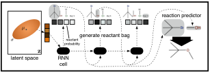
In this paper we propose a generative model for molecules (shown in Figure 1) that describes how to make such molecules from a set of commonly-available reactants. Our model first generates a set of reactant molecules, and second maps them to a predicted product molecule via a reaction prediction model. It allows one to simultaneously search for better molecules and describe how such molecules can be made. By closely mimicking the real-world process of designing new molecules, we show that our model: 1. Is able to generate a wide range of molecules not seen in the training data; 2. Addresses practical synthesis concerns such as reaction stability and toxicity; and 3. Allows us to propose new reactants for given target molecules that may be more practical to manage.

Refer to caption — Figure 1: An overview of approaches used to find molecules with desirable properties. *Left*: Virtual screening [52] aims to find novel molecules by the (computationally expensive) enumeration over all possible combinations of fragments. *Center*: More recent ML approaches, eg [15], aim to find useful, novel molecules by optimizing in a continuous latent space; however, there are no clues to whether (and how) these molecules can be synthesized. *Right*: We approach the generation of molecules through a multistage process mirroring how complex molecules are created in practice, while maintaining a continuous latent space to use for optimization. Our model, Molecule Chef, first finds suitable reactants which then react together to create a final molecule.

2 Background

We start with an overview of traditional computational techniques to discover novel molecules with desirable properties. We then review recent work in machine learning (ML) that seeks to improve parts of this process. We then identify aspects of molecule discovery we believe deserve much more attention from the ML community. We end by laying out our contributions to address these concerns.

2.1 Virtual Screening

To discover new molecules with certain properties, one popular technique is virtual screening (VS) [52, 18, 41, 8, 38]. VS works by (a) enumerating all combinations of a set of building-block molecules (which are combined via virtual chemical bonding rules), (b) for each molecule, calculating the desired properties via simulations or prediction models, (c) filtering the most interesting molecules to synthesize in the lab. While VS is general, it has the important downside that the generation process is not targeted: VS needs to get lucky to find molecules with desirable properties, it does not search for them. Given that the number of possible drug-like compounds is estimated to be $\in[10^{23},10^{100}]$ [56], the chemical space usually screened in VS $\in[10^{7},10^{10}]$ is tiny. Searching in combinatorial fragment spaces has been proposed, but is limited to simpler similarity queries [42].

2.2 The Molecular Search Problem

To address these downsides, one idea is to replace this full enumeration with a search algorithm; an idea called de novo-design (DND) [46]. Instead of generating a large set of molecules with small variations, DND searches for molecules with particular properties, recomputes them for the newfound molecules, and searches again. We call this the molecular search problem. Early work on the molecular search problem used genetic algorithms, ant-colony optimization, or other discrete search techniques to make local changes to molecules [17]. While more directed than library-generation, these approaches still explored locally, limiting the diversity of discovered molecules.

The first work to apply current ML techniques to this problem was Gómez-Bombarelli et al. 2018 (in a late 2016 preprint). Their idea was to search by learning a mapping from molecular space to continuous space and back. With this mapping it is possible to leverage well-studied optimization techniques to do search: local search can be done via gradient descent and global search via Bayesian optimization [54, 14]. For such a mapping, the authors chose to represent molecules as SMILES strings [58] and leverage advances in generative models for text [5] to learn a character variational autoencoder (CVAE) [29]. Shortly after this work, in an early 2017 preprint, Segler et al. 2017 trained recurrent neural networks (RNNs) to take properties as input and output SMILES strings with these properties, with molecular search done using reinforcement learning (RL).

In Search of Molecular Validity.

However, the SMILES string representation is very brittle: if individual characters are changed or swapped, it may no longer represent any molecule (called an invalid molecule). Thus, the CVAE often produced invalid molecules (in one experiment, Kusner et al. 2017 sampling from the continuous space, produced valid molecules only $0.7\%$ of the time). To address this validity problem, recent works have proposed using alternative molecular representations such as parse trees [30, 11] or graphs [53, 12, 32, 22, 33, 59, 23, 26, 45], where some of the more recent among these enforce or strongly encourage validity [22, 33, 59, 26, 45]. In parallel, there has been work based on RL that has aimed to learn a validity function during training directly [16, 20].

2.3 The Molecular Recipe Problem

Crucially, all of the works in the previous section solving the molecular search problem focus purely on optimizing molecules towards desirable properties. These works, in addressing the downsides of VS, removed a benefit of it: knowledge of the synthesis pathway of each molecule. Without this we do not know how practical it is to make ML-generated molecules.

To address this concern is to address the molecular recipe problem: what molecules are we able to make, given a set of readily-available starting molecules? So far, this problem has been addressed independently of the molecular search problem through synthesis planning (SP) [51]. SP works by recursively deconstructing a molecule. This deconstruction is done via (reversed) reaction predictors: models that predict how reactant molecules produce a product molecule. More recently, novel ML models have been designed for reaction prediction [57, 49, 21, 47, 6, 48].

2.4 This Work

In this paper, we propose to address both the molecular search problem and the molecular recipe problem jointly. To do so, we propose a generative model over molecules using the following map: First, a mapping from continuous space to a set of known, reliable, easy-to-obtain reactant molecules. Second a mapping from this set of reactant molecules to a final product molecule, based on a reaction prediction model [57, 49, 21, 48, 6]. Thus our generative model not only generates molecules, but also a synthesis route using available reactants. This addresses the molecular recipe problem, and also the molecular search problem, as the learned continuous space can also be used for search. Compared to previous work, in this work we are searching for new molecules through virtual chemical reactions, more directly simulating how molecules are actually discovered in the lab.

Concretely, we argue that our model, which we shall introduce in the next section, has several advantages over the current deep generative models of molecules reviewed previously:

Better extrapolation properties: Generating molecules through graph editing operations, representing reactions, we hope gives us strong inductive biases for extrapolating well.
Validity of generated molecules: Naive generation of molecular SMILES strings or graphs can lead to molecules that are invalid. Although the syntactic validity can be fixed by using masking [30, 33], the molecules generated can often still be semantically invalid. By generating molecules from chemically stable reactants by means of reactions, our model proposes more semantically valid molecules.
Provide synthesis routes: Proposed molecules from other methods can often not be evaluated in practice, as chemists do not know how to synthesize them. As a byproduct of our model we suggest synthetic routes, which could have a useful, practical value.

3 Model

In this section we describe our model¹¹ 1 Further details can also be found in our appendix and code is available at https://github.com/john-bradshaw/molecule-chef. We define the set of all possible valid molecular graphs as $\mathcal{G}$ , with an individual graph $g\in\mathcal{G}$ representing the atoms of a molecule as its nodes, and the type of bonds between these atoms (we consider single, double and triple bonds) as its edge types. The set of common reactant molecules, easily procurable by a chemist, which we want to act as building blocks for any final molecule is a subset of this, $\mathcal{R}\subset\mathcal{G}$ .

As discussed in the previous section (and shown in Figure 1) our generative model for molecules consists of the composition of two parts: (1) a decoder from a continuous latent space, $\mathbf{z}\in\mathbb{R}^{m}$ , to a bag (ie multiset²² 2 Note how we allow molecules to be present multiple times as reactants in our reaction, although practically many reactions only have one instance of a particular reactant.) of easily procurable reactants, $\mathbf{x}\subset\mathcal{R}$ ; (2) a reaction predictor model that transforms this bag of molecules into a multiset of product molecules $\mathbf{y}\subset\mathcal{G}$ .

The benefit of this approach is that for step (2) we can pick from several existing reaction predictor models, including recently proposed methods that have used ML techniques [27, 49, 48, 6, 10]. In this work we use the Molecular Transformer (MT) of Schwaller et al. 2019, as it has recently been shown to provide state-of-the-art performance in this task [48, Table 4].

This leaves us with the task of (1), learning a way to decode to (and encode from) a bag of reactants, using a parameterized encoder $q(\mathbf{z}|\mathbf{x})$ and decoder $p(\mathbf{x}|\mathbf{z})$ . We call this co-occurrence model Molecule Chef, and by moving around in the latent space we can select using Molecule Chef different “bags of reactants”.

Again there are several viable options of how to learn Molecule Chef. For instance one could choose to use a VAE for this task [29, 44]. However, when paired with a complex decoder these models are often difficult to train [5, 1], such that much of the previous work for generating graphs has has tuned down the KL regularization term in these models [33, 30]. We therefore instead propose using the WAE objective [55], which involves minimizing

\displaystyle L=

\displaystyle\mathbb{E}_{\mathbf{x}\sim\mathcal{D}}\mathbb{E}_{q(\mathbf{z}|\mathbf{x})}\left[c(\mathbf{x},p(\mathbf{x}|\mathbf{z}))\right]+\lambda D\left(\mathbb{E}_{\mathbf{x}\sim\mathcal{D}}\left[q(\mathbf{z}|\mathbf{x})\right],p(\mathbf{z})\right)

where $c$ is a cost function, that enforces the reconstructed bag to be similar to the encoded one. $D$ is a divergence measure, which is weighted in relative importance by $\lambda$ , that forces the marginalised distribution of all encodings to match the prior on the latent space. Following Tolstikhin et al. 2018 we use the maximum mean discrepancy (MMD) divergence measure, with $\lambda=10$ and a standard normal prior over the latents. We choose $c$ so that this first term matches the reconstruction term we would obtain in a VAE, i.e. with $c(\mathbf{x},\mathbf{z})=-\log p(\mathbf{x}|\mathbf{z})$ . This means that the objective only differs from a VAE in the second, regularisation term, such that we are not trying to match each encoding to the prior but instead the marginalised distribution over all datapoints. Empirically, we find that this trains well and does not suffer from the same local optimum issues as the VAE.

3.1 Encoder and Decoder

We can now begin describing the structure of our encoder and decoder. In these functions it is often convenient to work with $n$ -dimensional vector embeddings of graphs, $\mathbf{m}_{g}\in\mathbb{R}^{n}$ . Again we are faced with a series of possible alternative ways to compute these embeddings. For instance, we could ignore the structure of the molecular graph and learn a distinct embedding for each molecule, or use fixed molecular fingerprints, such as Morgan Fingerprints [37]. We instead choose to use deep graph neural networks [36, 13, 3] that can produce graph-isomorphic representations.

Deep graph neural networks have been shown to perform well on a variety of tasks involving small organic molecules, and their advantages compared to the previously mentioned alternative approaches are that (1) they take the structure of the graph into account and (2) they can learn which characteristics are important when forming higher-level representations. In particular in this work we use 4 layer Gated Graph Neural Networks (GGNN) [31]. These compute higher-level representations for each node. These node-level representations in turn can be combined by a weighted sum, to form a graph-level representation invariant to the order of the nodes, in an operation referred to as an aggregation transformation [24, §3].

Encoder

The structure of Molecule Chef’s encoder, $q(\mathbf{z}|\mathbf{x})$ , is shown in Figure 2. For the $i$ th data point the encoder has as input the multiset of reactants $\mathbf{x_{i}}=\{x^{i}_{1},x^{i}_{2},\cdots\}$ . It first computes the representation of each individual reactant molecule graph using the GGNN, before summing these representations to get a representation that is invariant to the order of the multiset. A feed forward network is then used to parameterize the mean and variance of a Gaussian distribution over $\mathbf{z}$ .

Decoder

The decoder, $p(\mathbf{x}|\mathbf{z})$ , (Figure 3) maps from the latent space to a multiset of reactant molecules. These reactants are typically small molecules, which means we could fit a deep generative model which produces them from scratch. However, to better mimic the process of selecting reactant molecules from an easily obtainable set, we instead restrict the output of the decoder to pick the molecules from a fixed set of reactant molecules, $\mathcal{R}$ .

This happens in a sequential process using a recurrent neural network (RNN), with the full process described in Algorithm 1. The latent vector, $\mathbf{z}$ is used to parametrize the initial hidden layer of the RNN. The selected reactants are fed back in as inputs to the RNN at the next generation stage. Whilst training we randomly sample the ordering of the reactants, and use teacher forcing.

Algorithm 1 Molecule Chef’s Decoder

\mathbf{z}^{i}

(latent space sample), GGNN (for embedding molecules), RNN (recurrent neural network),

\mathcal{R}

(set of easy-to-obtain reactant molecules),

\mathbf{s}

(learnt “halt” embedding),

\mathbf{A}

(learnt matrix that projects the size of the latent space to the size of RNN’s hidden space)

\mathbf{h}_{0}\leftarrow\mathbf{A}\mathbf{z}^{i}

;

\mathbf{m}_{0}\leftarrow\mathbf{0}

{Start symbol}

for

t=1

T_{\textrm{max}}

\mathbf{h}_{t}\leftarrow\textrm{RNN}(\mathbf{m}_{t-1},\mathbf{h}_{t-1})

;

\mathbf{B}\leftarrow

STACK([GGNN(g) for all g in

\mathcal{R}

] + [

\mathbf{s}

])

logits

\leftarrow\mathbf{h}_{t}\mathbf{B}^{T}

x_{t}\sim\textrm{softmax}(\textrm{logits})

x_{t}=\textrm{HALT}

then

break {If the logit corresponding to the halt embedding is selected then we stop early}

else

\mathbf{m}_{t}\leftarrow\textrm{GGNN}(x_{t})

end if

end for

return

x_{1},x_{2},\cdots

3.2 Adding a predictive penalty loss to the latent space

As discussed in section 2.2 we are interested in using and evaluating our model’s performance in the molecular search problem, that is using the learnt latent space to find new molecules with desirable properties. In reality we would wish to measure some complex chemical property that can only be measured experimentally. However, as a surrogate for this, following [15], we optimize instead for the QED (Quantitative Estimate of Drug-likeness [4]) score of a molecule, $\mathbf{w}$ , as a deterministic mapping from molecules to this score, $\mathbf{y}\mapsto\mathbf{w}$ , exists in RDKit [43].

To this end, in a similar manner to Liu et al. 2018 & Jin et al. 2018, we can simultaneously train a 2 hidden layer property predictor NN for use in local optimization tasks. This network tries to predict the QED property, $\mathbf{w}$ , of the final product $\mathbf{y}$ from the latent encoding of the associated bag of reactants. The use of this property predictor network for local optimization is described in Section 4.2.

4 Evaluation

In this section we evaluate Molecule Chef in (1) its ability to generate a diverse set of valid molecules; (2) how useful its learnt latent space is when optimizing product molecules for some property; and (3) whether by training a regressor back from product molecules to the latent space, Molecule Chef can be used as part of a setup to perform retrosynthesis.

In order to train our model we need a dataset of reactant bags. For this we use the USPTO dataset [34], processed and cleaned up by Jin et al. 2017. We filter out reagents, molecules that form context under which the reaction occurs but do not contribute atoms to the final products, by following the approach of Schwaller et al. 2018.

We wish to use as possible reactant molecules only popular molecules that a chemist would have easy access to. To this end, we filter our training (using Jin et al. 2017’s split) dataset so that each reaction only contains reactants that occur at least 15 times across different reactions in the original larger training USPTO dataset. This leaves us with a dataset of 34426 unique reactant bags for training the Molecule Chef. In total there are 4344 unique reactants. For training the baselines, we combine these 4344 unique reactants and the associated products from their different combinations, to form a training set for baselines, as even though Molecule Chef has not seen the products during training, the reaction predictor has.

4.1 Generation

We begin by analyzing our model using the metrics favored by previous work³³ 3 Note that we have extended the definition of these metrics to a bag (multiset) of products, given that our model can output multiple molecules for each reaction. However, when sampling 20000 times from the prior of our model, we generate single product bags 97% of the time, so that in practice most of the time we are using the same definition for these metrics as the previous work which always generated single molecules. [22, 33, 32, 30]: validity, uniqueness and novelty. Validity is defined as requiring that at least one of the molecules in the bag of products can be parsed by RDKit. For a bag of products to be unique we require it to have at least one valid molecule that the model has not generated before in any of the previously seen bags. Finally, for computing novelty we require that the valid molecules not be present in the same training set we use for the baseline generative models.

Table 1: Table showing the validity, uniqueness, novelty and normalized quality (all as %, higher better) of the products/or molecules generated from decoding from 20k random samples from the prior

p(\mathbf{z})

. Quality is the proportion of valid molecules that pass the quality filters proposed in Brown et al. 2019, normalized such that the score on the training set is 100. FCD is the Fréchet ChemNet Distance [40], capturing a notion of distance between the generated valid molecules and the training dataset (lower better). The uniqueness and novelty figures are also conditioned on validity. MT stands for the Molecular Transformer [48].

Model Name	Validity	Uniqueness	Novelty	Quality	FCD
Molecule Chef + MT	99.05	95.95	89.11	95.30	0.73
AAE [25, 39]	85.86	98.54	93.37	94.89	1.12
CGVAE [33]	100.00	93.51	95.88	44.45	11.73
CVAE [15]	12.02	56.28	85.65	52.86	37.65
GVAE [30]	12.91	70.06	87.88	46.87	29.32
LSTM [50]	91.18	93.42	74.03	100.12	0.43

In addition, we compute the Fréchet ChemNet Distance (FCD) [40] between the valid molecules generated by each method and our baseline training set. Finally in order to try to assess the quality of the molecules generated we record the (train-normalized) proportion of valid molecules that pass the quality filters proposed by Brown et al. 2019; these filters aim to remove molecules that are “potentially unstable, reactive, laborious to synthesize, or simply unpleasant to the eye of medicinal chemists”.

For the baselines we consider the character VAE (CVAE) [15], the grammar VAE (GVAE) [30], the AAE (adversarial autoencoder) [25], the constrained graph VAE (CGVAE) [33], and a stacked LSTM generator with no latent space [50]. Further details about the baselines can be found in the appendix.

The results are shown in Table 1. As Molecule Chef decodes to a bag made up from a predefined set of molecules, those reactants going into the reaction predictor are valid. The validity of the final product is not 100%, as the reaction predictor can make non-valid edits to these molecules, but we see that in a high number of cases the products are valid too. Furthermore, what is very encouraging is that the molecules generated often pass the quality filters, giving evidence that the process of building molecules up by combining stable reactant building blocks often leads to stable products.

4.2 Local Optimization

As discussed in Section 3.2, when training Molecule Chef we can simultaneously train a property predictor network, mapping from the latent space of Molecule Chef to the QED score of the final product. In this section we look at using the gradient information obtainable from this network to do local optimization to find a molecule created from our reactant pool that has a high QED score.

We evaluate the local optimization of molecular properties by taking 250 bags of reactants, encoding them into the latent space of Molecule Chef, and then repeatedly moving in the latent space using the gradient direction of the property predictor until we have decoded ten different reactant bags. As a comparison we consider instead moving in a random walk until we have also decoded to ten different reaction bags. In Figure 4 we look at the distribution of the best QED score found in considering these ten reactant bags, and how this compared to the QEDs started with.

Figure 4: KDE plot showing that the distribution of the best QEDs found through local optimization, using our trained property predictor for QEDs, has higher mass over higher QED scores compared to the best found from a random walk. The starting locations’ distribution (sampled from the training data) is shown in green. The final products, given a reactant bag are predicted using the MT [48].

Figure 5: Having learnt a latent space which can map to products through reactants, we can learn a regressor back from the suggested products to the latent space (orange dashed

--

arrow shown) and couple this with Molecule Chef’s decoder to see if we can do retrosynthesis – the act of computing the reactants that create a particular product.

When looking at individual optimization runs, we see that the QEDs vary a lot between different products even if made with similar reactants. However, Figure 4 shows that overall the distribution of the final best found QED scores is improved when purposefully optimizing for this. This is encouraging as it gives evidence of the utility of these models for the molecular search problem.

4.3 Retrosynthesis

A unique feature of our approach is that we learn a decoder from latent space to a bag of reactants. This gives us the ability to do retrosynthesis by training a model to map from products to their associated reactants’ representation in latent space and using this in addition to Molecule Chef’s decoder to generate a bag of reactants. This process is highlighted in Figure 5. Although retrosynthesis is a difficult task, with often multiple possible ways to create the same product and with current state-of-the-art approaches built using large reaction databases and able to deal with multiple reactions [51], we believe that our model could open up new interesting and exciting approaches to this task. We therefore train a small network based on the same graph neural network structure used for Molecule Chef followed by four fully connected layers to regress from products to latent space.

Figure 6: An example of performing retrosynthesis prediction using a trained regressor from products to latent space. This reactant-product pair has not been seen in the training set of Molecule Chef. Further examples are shown in the appendix.

(a) Reachable Products

(b) Unreachable Products

Figure 7: Assessing the correlation between the QED scores for the original product and its reconstruction (see text for details). We assess on two portions of the test set, products that are made up of only reactants in Molecule Chef’s vocabulary are called ‘Reachable Products’, those that have at least one reactant that is absent are called ‘Unreachable Products’.

A few examples of the predicted reactants corresponding to products from reactions in the USPTO test set, but which can be made in one step from the predefined possible reactants, are shown in Figure 6 and the appendix. We see that often this approach, although not always able to suggest the correct whole reactant bag, chooses similar reactants that on reaction produce similar structures to the original product we were trying to synthesize. While we would not expect this approach to retrosynthesis to be competitive with complex planning tools, we think this provides a promising new approach, which could be used to identify bags of reactants that produce molecules similar to a desired target molecule. In practice, it would be valuable to be pointed directly to molecules with similar properties to a target molecule if they are easier to make than the target, since it is the properties of the molecules, and not the actual molecules themselves, that we are after.

With this in mind, we assess our approach in the following way: (1) we take a product and perform retrosynthesis on it to produce a bag of reactants, (2) we transform this bag of reactants using the Molecular Transformer to produce a new reconstructed product, and then finally (3) we plot the resulting reconstructed product molecule’s QED score against the QED score of the initial product. We evaluate on a filtered version of Jin et al. 2017’s test set split of USPTO, where we have filtered out any reactions which have the exact same reactant and product multisets as a reaction present in the set used to train Molecule Chef. In addition, we further split this filtered set into two sets: (i) ‘Reachable Products’, which are reactions in the test set that contain as reactants only molecules that are in Molecule Chef’s reactant vocabulary, and (ii) ‘Unreachable Products’, which have at least one reactant molecule that is not in the vocabulary.

The results are shown in Figure 7; overall we see that there is some correlation between the properties of products and the properties of their reconstructions. This is more prominent for the reachable products, which we believe is because our latent space is only trained on reachable product reactions and so is better able to model these reactions. Furthermore, some of the unreachable products may also require reactants that are not available in our pool of easily available reactants, at least when considering one-step reactions. However, given that unreachable products have at least one reactant which is not in Molecule Chef’s vocabulary, we think it is very encouraging that there still is some, albeit smaller, correlation with the true QED. This is because it shows that our model can suggest molecules with similar properties made from reactants that are available.

4.4 Qualitative Quality of Samples

In Figure 8 we show molecules generated from a random walk starting from the encoding of a particular molecule (shown in the left-most column). We compare the CVAE, GVAE, and Molecule Chef (for Molecule Chef we encode the reactant bag known to generate the same molecule). We showed all generated molecules to a domain expert and asked them to evaluate their properties in terms of their stability, toxicity, oxidizing power, corrosiveness (the rationales are provided in more detail in the Appendix). Many molecules produced by the CVAE and GVAE show undesirable features, unlike the molecules generated by Molecule Chef.

5 Discussion

In this work we have introduced Molecule Chef, a model that generates synthesizable molecules, by considering the products produced as a result of one-step reactions from a pool of pre-defined reactants. By constructing molecules through selecting reactants and running chemical reactions, while performing optimization in a continuous latent space, we can combine the strengths of previous VAE-based models and classical discrete de-novo design algorithms based on virtual reactions. As future work, we hope to explore how to extend our approach to deal with larger reactant vocabularies and multi-step reactions. This would allow the generation of a wider range of molecules, whilst maintaining our approach’s advantages of being able to suggest synthetic routes and often producing semantically valid molecules.

Acknowledgements

This work was supported by The Alan Turing Institute under the EPSRC grant EP/N510129/1. JB also acknowledges support from an EPSRC studentship.

References

Alemi et al. [2018] Alexander Alemi, Ben Poole, Ian Fischer, Joshua Dillon, Rif A Saurous, and Kevin Murphy. Fixing a broken ELBO. In International Conference on Machine Learning, pages 159–168, 2018.
Assouel et al. [2018] Rim Assouel, Mohamed Ahmed, Marwin H Segler, Amir Saffari, and Yoshua Bengio. Defactor: Differentiable edge factorization-based probabilistic graph generation. arXiv preprint arXiv:1811.09766, 2018.
Battaglia et al. [2018] Peter W Battaglia, Jessica B Hamrick, Victor Bapst, Alvaro Sanchez-Gonzalez, Vinicius Zambaldi, Mateusz Malinowski, Andrea Tacchetti, David Raposo, Adam Santoro, Ryan Faulkner, et al. Relational inductive biases, deep learning, and graph networks. arXiv preprint arXiv:1806.01261, 2018.
Bickerton et al. [2012] G Richard Bickerton, Gaia V Paolini, Jérémy Besnard, Sorel Muresan, and Andrew L Hopkins. Quantifying the chemical beauty of drugs. Nature chemistry, 4(2):90, 2012.
Bowman et al. [2016] Samuel R Bowman, Luke Vilnis, Oriol Vinyals, Andrew M Dai, Rafal Jozefowicz, and Samy Bengio. Generating sentences from a continuous space. In Proceedings of The 20th SIGNLL Conference on Computational Natural Language Learning, 2016.
Bradshaw et al. [2019] John Bradshaw, Matt J Kusner, Brooks Paige, Marwin HS Segler, and José Miguel Hernández-Lobato. A generative model for electron paths. In International Conference on Learning Representations, 2019.
Brown et al. [2019] Nathan Brown, Marco Fiscato, Marwin H.S. Segler, and Alain C. Vaucher. Guacamol: Benchmarking models for de novo molecular design. Journal of Chemical Information and Modeling, 59(3):1096–1108, 2019. doi: 10.1021/acs.jcim.8b00839.
Chevillard and Kolb [2015] Florent Chevillard and Peter Kolb. Scubidoo: A large yet screenable and easily searchable database of computationally created chemical compounds optimized toward high likelihood of synthetic tractability. J. Chem. Inf. Mod., 55(9):1824–1835, 2015.
Cho et al. [2014] Kyunghyun Cho, Bart van Merriënboer, Caglar Gulcehre, Dzmitry Bahdanau, Fethi Bougares, Holger Schwenk, and Yoshua Bengio. Learning phrase representations using RNN encoder–decoder for statistical machine translation. In Proceedings of the 2014 Conference on Empirical Methods in Natural Language Processing (EMNLP), pages 1724–1734, Doha, Qatar, October 2014. Association for Computational Linguistics. doi: 10.3115/v1/D14-1179. URL https://www.aclweb.org/anthology/D14-1179.
Coley et al. [2019] Connor W Coley, Wengong Jin, Luke Rogers, Timothy F Jamison, Tommi S Jaakkola, William H Green, Regina Barzilay, and Klavs F Jensen. A graph-convolutional neural network model for the prediction of chemical reactivity. Chemical Science, 10(2):370–377, 2019.
Dai et al. [2018] Hanjun Dai, Yingtao Tian, Bo Dai, Steven Skiena, and Le Song. Syntax-directed variational autoencoder for structured data. In International Conference on Learning Representations, 2018.
De Cao and Kipf [2018] Nicola De Cao and Thomas Kipf. MolGAN: An implicit generative model for small molecular graphs. In International Conference on Machine Learning Deep Generative Models Workshop, 2018.
Duvenaud et al. [2015] David K Duvenaud, Dougal Maclaurin, Jorge Iparraguirre, Rafael Bombarell, Timothy Hirzel, Alán Aspuru-Guzik, and Ryan P Adams. Convolutional networks on graphs for learning molecular fingerprints. In Advances in neural information processing systems, pages 2224–2232, 2015.
Gardner et al. [2014] Jacob R Gardner, Matt J Kusner, Zhixiang Eddie Xu, Kilian Q Weinberger, and John P Cunningham. Bayesian optimization with inequality constraints. In International Conference on Machine Learning, pages 937–945, 2014.
Gómez-Bombarelli et al. [2018] Rafael Gómez-Bombarelli, Jennifer N Wei, David Duvenaud, José Miguel Hernández-Lobato, Benjamín Sánchez-Lengeling, Dennis Sheberla, Jorge Aguilera-Iparraguirre, Timothy D Hirzel, Ryan P Adams, and Alán Aspuru-Guzik. Automatic chemical design using a Data-Driven continuous representation of molecules. ACS Cent Sci, 4(2):268–276, February 2018.
Guimaraes et al. [2017] Gabriel Lima Guimaraes, Benjamin Sanchez-Lengeling, Carlos Outeiral, Pedro Luis Cunha Farias, and Alán Aspuru-Guzik. Objective-reinforced generative adversarial networks (ORGAN) for sequence generation models. arXiv preprint arXiv:1705.10843, 2017.
Hartenfeller and Schneider [2011] Markus Hartenfeller and Gisbert Schneider. Enabling future drug discovery by de novo design. Wiley Interdisc. Rev. Comp. Mol. Sci., 1(5):742–759, 2011.
Hu et al. [2011] Qiyue Hu, Zhengwei Peng, Jaroslav Kostrowicki, and Atsuo Kuki. Leap into the Pfizer global virtual library (PGVL) space: creation of readily synthesizable design ideas automatically. In Chemical Library Design, pages 253–276. Springer, 2011.
Irwin et al. [2012] John J Irwin, Teague Sterling, Michael M Mysinger, Erin S Bolstad, and Ryan G Coleman. ZINC: a free tool to discover chemistry for biology. Journal of chemical information and modeling, 52(7):1757–1768, 2012.
Janz et al. [2018] David Janz, Jos van der Westhuizen, Brooks Paige, Matt J Kusner, and José Miguel Hernández-Lobato. Learning a generative model for validity in complex discrete structures. In International Conference on Learning Representations, 2018.
Jin et al. [2017] Wengong Jin, Connor W Coley, Regina Barzilay, and Tommi Jaakkola. Predicting organic reaction outcomes with Weisfeiler-Lehman network. In Advances in Neural Information Processing Systems, 2017.
Jin et al. [2018] Wengong Jin, Regina Barzilay, and Tommi Jaakkola. Junction tree variational autoencoder for molecular graph generation. In International Conference on Machine Learning, 2018.
Jin et al. [2019] Wengong Jin, Kevin Yang, Regina Barzilay, and Tommi Jaakkola. Learning multimodal graph-to-graph translation for molecular optimization. In International Conference on Learning Representations, 2019.
Johnson [2017] Daniel D Johnson. Learning graphical state transitions. In International Conference on Learning Representations, 2017.
Kadurin et al. [2017] Artur Kadurin, Alexander Aliper, Andrey Kazennov, Polina Mamoshina, Quentin Vanhaelen, Kuzma Khrabrov, and Alex Zhavoronkov. The cornucopia of meaningful leads: Applying deep adversarial autoencoders for new molecule development in oncology. Oncotarget, 8(7):10883, 2017.
Kajino [2019] Hiroshi Kajino. Molecular hypergraph grammar with its application to molecular optimization. In International Conference on Machine Learning, pages 3183–3191, 2019.
Kayala et al. [2011] Matthew A Kayala, Chloé-Agathe Azencott, Jonathan H Chen, and Pierre Baldi. Learning to predict chemical reactions. Journal of chemical information and modeling, 51(9):2209–2222, 2011.
Kingma and Ba [2015] Diederik Kingma and Jimmy Ba. Adam: A method for stochastic optimization. In International Conference on Learning Representations, 2015.
Kingma and Welling [2014] Diederik P Kingma and Max Welling. Auto-encoding variational Bayes. In International Conference on Learning Representations, 2014.
Kusner et al. [2017] Matt J Kusner, Brooks Paige, and José Miguel Hernández-Lobato. Grammar variational autoencoder. In International Conference on Machine Learning, 2017.
Li et al. [2016] Yujia Li, Daniel Tarlow, Marc Brockschmidt, and Richard Zemel. Gated graph sequence neural networks. International Conference on Learning Representations, 2016.
Li et al. [2018] Yujia Li, Oriol Vinyals, Chris Dyer, Razvan Pascanu, and Peter Battaglia. Learning deep generative models of graphs. arXiv preprint arXiv:1803.03324, March 2018.
Liu et al. [2018] Qi Liu, Miltiadis Allamanis, Marc Brockschmidt, and Alexander L Gaunt. Constrained graph variational autoencoders for molecule design. In Advances in neural information processing systems, 2018.
Lowe [2012] Daniel Mark Lowe. Extraction of chemical structures and reactions from the literature. PhD thesis, University of Cambridge, 2012.
Mayr et al. [2018] Andreas Mayr, Günter Klambauer, Thomas Unterthiner, Marvin Steijaert, Jörg K. Wegner, Hugo Ceulemans, Djork-Arné Clevert, and Sepp Hochreiter. Large-scale comparison of machine learning methods for drug target prediction on chembl. Chem. Sci., 9:5441–5451, 2018. doi: 10.1039/C8SC00148K. URL http://dx.doi.org/10.1039/C8SC00148K.
Merkwirth and Lengauer [2005] Christian Merkwirth and Thomas Lengauer. Automatic generation of complementary descriptors with molecular graph networks. Journal of chemical information and modeling, 45(5):1159–1168, 2005.
Morgan [1965] HL Morgan. The generation of a unique machine description for chemical structures-a technique developed at chemical abstracts service. Journal of Chemical Documentation, 5(2):107–113, 1965.
Nicolaou et al. [2016] Christos A Nicolaou, Ian A Watson, Hong Hu, and Jibo Wang. The proximal lilly collection: Mapping, exploring and exploiting feasible chemical space. Journal of chemical information and modeling, 56(7):1253–1266, 2016.
Polykovskiy et al. [2018] Daniil Polykovskiy, Alexander Zhebrak, Benjamin Sanchez-Lengeling, Sergey Golovanov, Oktai Tatanov, Stanislav Belyaev, Rauf Kurbanov, Aleksey Artamonov, Vladimir Aladinskiy, Mark Veselov, Artur Kadurin, Sergey Nikolenko, Alan Aspuru-Guzik, and Alex Zhavoronkov. Molecular Sets (MOSES): A Benchmarking Platform for Molecular Generation Models. arXiv preprint arXiv:1811.12823, 2018.
Preuer et al. [2018] Kristina Preuer, Philipp Renz, Thomas Unterthiner, Sepp Hochreiter, and Günter Klambauer. Fréchet chemnet distance: A metric for generative models for molecules in drug discovery. Journal of Chemical Information and Modeling, 58(9):1736–1741, 2018. doi: 10.1021/acs.jcim.8b00234.
Pyzer-Knapp et al. [2015] Edward O Pyzer-Knapp, Changwon Suh, Rafael Gómez-Bombarelli, Jorge Aguilera-Iparraguirre, and Alán Aspuru-Guzik. What is high-throughput virtual screening? A perspective from organic materials discovery. Annual Review of Materials Research, 45:195–216, 2015.
Rarey and Stahl [2001] Matthias Rarey and Martin Stahl. Similarity searching in large combinatorial chemistry spaces. Journal of Computer-Aided Molecular Design, 15(6):497–520, 2001.
[43] RDKit, online. RDKit: Open-source cheminformatics. http://www.rdkit.org. [Online; accessed 01-February-2018].
Rezende et al. [2014] Danilo Jimenez Rezende, Shakir Mohamed, and Daan Wierstra. Stochastic backpropagation and approximate inference in deep generative models. In International Conference on Machine Learning, pages 1278–1286, 2014.
Samanta et al. [2019] Bidisha Samanta, DE Abir, Gourhari Jana, Pratim Kumar Chattaraj, Niloy Ganguly, and Manuel Gomez Rodriguez. NeVAE: A deep generative model for molecular graphs. In Proceedings of the AAAI Conference on Artificial Intelligence, volume 33, pages 1110–1117, 2019.
Schneider and Schneider [2016] Petra Schneider and Gisbert Schneider. De novo design at the edge of chaos: Miniperspective. J. Med. Chem., 59(9):4077–4086, 2016.
Schwaller et al. [2018] Philippe Schwaller, Théophile Gaudin, Dávid Lányi, Costas Bekas, and Teodoro Laino. “Found in Translation”: predicting outcomes of complex organic chemistry reactions using neural sequence-to-sequence models. Chem. Sci., 9:6091–6098, 2018. doi: 10.1039/C8SC02339E.
Schwaller et al. [2019] Philippe Schwaller, Teodoro Laino, Théophile Gaudin, Peter Bolgar, Christopher A. Hunter, Costas Bekas, and Alpha A. Lee. Molecular transformer: A model for uncertainty-calibrated chemical reaction prediction. ACS Central Science, 5(9):1572–1583, 2019. doi: 10.1021/acscentsci.9b00576.
Segler and Waller [2017] Marwin HS Segler and Mark P Waller. Neural-symbolic machine learning for retrosynthesis and reaction prediction. Chemistry–A European Journal, 23(25):5966–5971, 2017.
Segler et al. [2017] Marwin HS Segler, Thierry Kogej, Christian Tyrchan, and Mark P Waller. Generating focused molecule libraries for drug discovery with recurrent neural networks. ACS Cent. Sci., 4(1):120–131, 2017.
Segler et al. [2018] Marwin HS Segler, Mike Preuss, and Mark P Waller. Planning chemical syntheses with deep neural networks and symbolic AI. Nature, 555(7698):604, 2018.
Shoichet [2004] Brian K Shoichet. Virtual screening of chemical libraries. Nature, 432(7019):862, 2004.
Simonovsky and Komodakis [2018] Martin Simonovsky and Nikos Komodakis. GraphVAE: Towards generation of small graphs using variational autoencoders. In Věra Kůrková, Yannis Manolopoulos, Barbara Hammer, Lazaros Iliadis, and Ilias Maglogiannis, editors, Artificial Neural Networks and Machine Learning – ICANN 2018, pages 412–422, Cham, 2018. Springer International Publishing. ISBN 978-3-030-01418-6.
Snoek et al. [2012] Jasper Snoek, Hugo Larochelle, and Ryan P Adams. Practical Bayesian optimization of machine learning algorithms. In Advances in neural information processing systems, pages 2951–2959, 2012.
Tolstikhin et al. [2018] Ilya Tolstikhin, Olivier Bousquet, Sylvain Gelly, and Bernhard Schoelkopf. Wasserstein auto-encoders. In International Conference on Learning Representations, 2018.
van Hilten et al. [2019] Niek van Hilten, Florent Chevillard, and Peter Kolb. Virtual compound libraries in computer-assisted drug discovery. Journal of chemical information and modeling, 2019.
Wei et al. [2016] Jennifer N Wei, David Duvenaud, and Alán Aspuru-Guzik. Neural networks for the prediction of organic chemistry reactions. ACS central science, 2(10):725–732, 2016.
Weininger [1988] David Weininger. SMILES, a chemical language and information system. 1. Introduction to methodology and encoding rules. Journal of chemical information and computer sciences, 28(1):31–36, 1988.
You et al. [2018] Jiaxuan You, Bowen Liu, Rex Ying, Vijay Pande, and Jure Leskovec. Graph convolutional policy network for goal-directed molecular graph generation. In Advances in Neural Information Processing Systems, 2018.

Appendix A Appendix

A.1 Generation Benchmarks on ZINC

We also ran the baselines for the generation task on the ZINC dataset [19]. The results are shown in Table 2.

Table 2: Table showing generation results for the baseline models when trained on ZINC dataset [19]. The first four result columns show the validity, uniqueness, novelty and normalized quality (all as %, higher better) of the molecules generated from decoding from 20k random samples from the prior

p(\mathbf{z})

. Quality is the proportion of molecules that pass the quality filters proposed in Brown et al. 2019, normalized such that the score on the USPTO derived training dataset (used in the main paper) is 100. FCD is the Fréchet ChemNet Distance [40], capturing a notion of distance between the generated molecules and the USPTO derived training dataset used in the main paper.

Model Name	Validity	Uniqueness	Novelty	Quality	FCD
AAE [25, 39]	87.64	100.00	99.99	96.12	7.27
CGVAE [33]	100.00	95.39	96.54	43.48	15.30
CVAE [15]	0.31	40.98	24.59	128.54	40.10
GVAE [30]	3.66	85.23	95.08	38.86	27.31
LSTM [50]	95.71	99.98	99.93	108.68	7.99

A.2 Further Random Walk Examples and Rationales for Expert Annotation

Rationales for expert labels in Figure 9 in the main text.

Denoted using letters for letters for rows and numbers for columns. A3: Unstable, enol; A5: unstable, aminal; B2: reactive, radical; B4: unstable ring system; B5: toxic, reactive sulfur-chloride bond, unstable ring system; B6: unstable ring system; B7: unstable ring system; B9: toxic: thioketone.

A.3 Further Retrosynthesis Results

In this section we first provide more retrosynthesis examples before also describing an extra experiment in which we try to assess how well the retrosynthesis pipeline is at finding molecules with similar properties, even if not reconstructing the correct reactants themselves.

A.3.1 Further Examples

(a)

(b)

(c)

(d)

Figure 11: Further examples of the predicted reactants associated with a given product for product molecules not in Molecule Chef’s training dataset, however with reactants belonging to Molecule Chef’s vocabulary (ie Reachable Dataset).

(a)

(b)

Figure 12: Further examples of the predicted reactants associated with a given product for product molecules not in Molecule Chef’s training dataset, with at least one reactants not part of Molecule Chef’s vocabulary (ie Unreachable Dataset).

A.3.2 ChemNet Distances between Products and their Reconstructions

We also consider an experiment for which we analyze the Euclidean distance between the ChemNet embeddings of the product and the reconstructed product (found by feeding the original product through our retrosynthesis pipeline and then the Molecular Transformer). ChemNet embeddings are used when calculating the FCD score [40] between molecule distributions, and so hopefully capture various properties of the molecule [35]. Whilst learning Molecule Chef we include a NN regressor from the latent space to the associated ChemNet embeddings, for which the MSE loss is minimized during training.

To try to establish an idea of how randomly chosen pairs of molecules in our dataset differ from each other, when measured using this metric, we provide a distribution of the distances of random pairs. This distribution is formed by taking each of the molecules in our dataset (consisting of all the reactants and their associated products) and matching it up with another randomly chosen molecule from this set, before measuring the Euclidean distance between the embeddings of each of these pairs.

The results are shown in Figure 13. We see that the distribution of distances between the products and their reconstructions has greater mass on smaller distances compared to the random pairs baseline.

(a) When evaluated on the portion of USPTO test set reactions for which both reactants are present in the Molecule Chef’s vocabulary.

(b) When evaluated on the portion of USPTO test set reactions for which at least one reactant is not present in the Molecule Chef’s vocabulary.

Figure 13: KDE plot showing the distribution of the Euclidean distances between the ChemNet embeddings [40] of our product and reconstructed product.

A.4 Details about our Dataset

In this section we provide further details about the molecules used in training our model and the baselines. We also describe details of the molecules used in the retrosynthesis experiments.

For Molecule Chef’s vocabulary we use reactants that occur at least 15 times in the USPTO train dataset, as processed and split by Jin et al. 2017. This dataset uses reactions collected by Lowe 2012 from USPTO patents. In total we have 4344 reactants, and a training set of 34426 unique reactant bags for which these reactants co-occur. Each reactant bag is associated with a product.

For the baselines we train on these reactants and the associated products. This results in a dataset of approximately 37000 unique molecules, containing a wide variety of heavy elements:

{’Al’, ’B’, ’Br’, ’C’, ’Cl’, ’Cr’, ’Cu’, ’F’, ’I’, ’K’, ’Li’, ’Mg’, ’Mn’, ’N’, ’Na’, ’O’, ’P’, ’S’, ’Se’, ’Si’, ’Sn’, ’Zn’ } .

Some examples of the molecules found in the dataset are shown in Figure 14. Note that the large number of heavy atoms present, as well as the small overall dataset size, makes a challenging learning task compared to when using some of the more common benchmark datasets used elsewhere (such as ZINC [19]).

Figure 14: Examples of molecules found in the dataset we use for training the baselines. This is a subset of the molecules found in USPTO [34]. It consists of the reactants that the Molecule Chef can produce along with their corresponding products. It contains complex molecules with challenging structures to learn.

We use examples from the USPTO test dataset when performing the retrosynthesis experiments. However, we first filter out any reactions for which the exact same reactant/product multisets tuple is also present in the training data for Molecule Chef ⁴⁴ 4 After canonicalisation and the removal of reagents, the USPTO train and test dataset has some reactions present in both sets.. Then we split the resultant dataset into two subsets. The first, which we refer to as the reachable dataset, contains only reactants in Molecule Chef’s vocabulary. The second, which we refer to as the unreachable dataset contains reactions with at least one reactant not in the vocabulary.

A.5 Implementation Details

Details of Molecule Chef’s architecture and parameters

An overview of Molecule Chef’s architrecture can be seen in Figure 15. The encoder takes in a multiset of reactants and outputs the parameters of a Gaussian distribution over $\bm{z}$ . The decoder maps from the latent space to a multiset of reactant molecules. Both of these networks rely in turn on vector representations of molecules computed by a graph neural network. We provide details of these networks’ architectures below as well as training details. Further information can be found in our code available at https://github.com/john-bradshaw/molecule-chef.

Figure 15: Overview of Molecule Chef showing how the encoder and decoder fit together.

Computing vector representations of molecular graphs using graph neural networks

For computing the vector representation of molecular graphs we used Gated Graph Neural Networks [31], with the same network shared in both the encoder and decoder. We run these networks for 4 propagation steps and the node representations have a dimension of 101. We initialise the node reprsentations with the atom features shown in Table 3. The final step’s node representation is projected down to a dimension of 50 by using a learnt linear projection. Graph level representations are formed from these node representations by performing a weighted sum.

Table 3: Atom features we use as input to the GGNN. These are calculated using RDKit.

Feature	Description
Atom type	72 possible elements in total, one hot
Degree	One hot (0, 1, 2, 3, 4, 5, 6, 7, 10)
Explicit Valence	One hot (0, 1, 2, 3, 4, 5, 6, 7, 8, 10, 12, 14)
Hybridization	One hot (SP, SP2, SP3, Other)
H count	integer
Electronegativity	float
Atomic number	integer
Part of an aromatic ring	boolean

Encoder

The encoder sums the vector representations of the molecules present in the reactant multiset to get a 50 dimensional vector representation of the entire multiset. This representation is fed through a single hidden layer NN (with a hidden layer size of 200) to parameterise the mean and diagonal of the covariance matrix of a 25 dimensional multivariate-Gaussian distribution over $\bm{z}$ .

Decoder

The decoder maps from the the latent space, $\bm{z}$ , to a multiset of reactants. It does this through a sequential process, selecting one reactant at a time using a gated recurrent unit (GRU) [9] RNN. The parameters used for this GRU are shown in Table 4. The initial hidden state of the RNN is set using the result from a learnt linear projection of $\bm{z}$ . The final output of the GRU is fed through a single hidden layer NN (with a hidden size of 128) to form a final output vector. The dot product of this final output vector is formed with each of the possible reactant embeddings as well as the HALT embedding to form logits for the next output of the decoder. The embedding of the reactant selected is fed back in as input into the RNN at the next step.

Table 4: Parameters for GRU used in decoder

Parameter	Value
GRU hidden size	50
GRU number of layers	2
GRU maximum number of steps	5

Property Predictor

In §3.2 of the main paper we discuss how we also can train a property predictor from the latent space to a property of interest such as the QED, while traing the WAE. For the QED property predictor NN we use a fully connected network with two hidden layers, both with dimensionality of 40. The loss from this network is added to the WAE loss when training the model for the local optimization and retrosynthesis tasks.

Training

We train the WAE (and property predictor when applicable) for 100 epochs. We use the Adam optimizer [28], with an initial learning rate of 0.001. We decay the learning rate by a factor of 10 every 40 epochs.

Implementation Details for the Baselines in Section 4.1 of Main Paper

For the baselines in the generation section in the main paper we use the following implementations:

•

CGVAE [33]: https://github.com/microsoft/constrained-graph-variational-autoencoder
•

LSTM [50], : https://github.com/BenevolentAI/guacamol_baselines
•

AAE [25, 39]: https://github.com/molecularsets/moses/tree/master/moses/aae
•

GVAE [30]: https://github.com/mkusner/grammarVAE
•

CVAE [15]: https://github.com/mkusner/grammarVAE

The LSTM baseline implementation follows Segler et al. 2017, which has as its alphabet a list of all individual element symbols, plus special characters used in SMILES strings. This differs from the alphabet used by the decoder in the Molecular Transformer [48], which instead extracts “bracketed” atoms directly from the training set; this means that a portion of a SMILES string such as [OH+] or [NH2-] would be represented as a single symbol, rather than as a sequence of five symbols. A regular expression can be used to extract a list of all such sequences from the training data. Effectively, this makes the trade off of increasing the alphabet size (from 47 to 203 items), while reducing the chance of making syntax errors or suggesting invalid charges. In practice we found very little qualitative or quantitative difference in the performance of the LSTM model for the two alphabets; for sake of consistency with Molecule Chef we report the baseline using the larger alphabet.

For the CGVAE we decide to include element-charge-valence triplets that occur at least 10 times over all the molecules in the training data. At generation time we pick one starting node at random.

Other Details

The majority of the experiments for Molecule Chef were run on a NVIDIA Tesla K80 GPU. For running the Molecular Transformer and CGVAE, we used NVIDIA P100 and P40 GPUs, as the latter in particular required a large memory GPU for training on the larger datasets.

For Molecule Chef we have not tried a wide range of hyperparameters. For the latent dimensionality we initially tried a dimension of 100 before trying and sticking with 25. Initially, we did not anneal the learning rate but found slightly improved performance by annealing it by a factor of 10 after 40 epochs. These changes were made after considering the reconstruction error of the model on the validation set (the validation dataset of USPTO restricted to the reactants in Molecule Chef’s vocabulary).