Elastic propagation of fast electron vortices through amorphous materials

The study of electron vortex beams (EVBs) is a highly active field of research in the context of transmission electron microscopy (TEM). The fact that these EVBs carry orbital angular momentum (OAM) has lead to many demonstrated and proposed applications ranging from the measurement of magnetic properties with atomic resolution [N_v467_i7313_p301, PRB_v89_i_p134428, U_v136_i_p81, ASaCI_v2_p5, U_v179_i_p15] over the study of the dynamics of Landau states [NC_v5_i_p4586, U_v158_i_p17], sample chirality [PRB_v91_i9_p94112], and symmetry properties of plasmon resonances [Nc_v8_i_p14999] to the manipulation of nanoparticles [AM_v25_i8_p1114]. Despite their huge potential and although their creation and propagation through vacuum is well-understood [U_v111_i9-10_p1461, U_v115_i0_p21, U_v158_i_p17], the knowledge of their propagation through matter is still somewhat lacking. This is especially surprising since earlier studies showed that elastic scattering in crystals can drastically change the orbital angular momentum of the beam [ACA_v68_i_p443, MaM_v18_i_p711, PRA_v87_i_p33834].

Particularly important — and little investigated — is the propagation of EVBs through amorphous materials. Firstly, such materials are used increasingly often for producing EVBs by means of specially designed phase masks [NJoP_v16_i_p93039, U_v144_i_p26, APL_v104_i4_p43109]. Secondly, they are a common support, e.g. for nanoparticles. Thirdly, EVBs would allow techniques such as energy-loss magnetic chiral dichroism (EMCD) for measuring magnetic properties down to the nanoscale in crystalline samples to be applied also to amorphous materials. However, it is usually assumed that an as-produced, ideal vortex beam stays that way and propagates practically unperturbed through the sample. Whether or not that is the case and, if so, to what extent is studied in this work.

This paper is structured as follows: first, we give a brief overview over the theory in sec. 2. To that end, we rewrite the multislice approach used throughout this work in a cylindrical coordinate system suitable for the analysis of EVBs. From that, we deduce some general statements about the propagation behavior of EVBs. In sec. 3, we give a detailed account of the numerical simulations performed in this work. In sec. 4, the results of the numerical simulations are presented, which are subsequently discussed in sec. 5.

The starting point for describing the propagation of electrons through matter is Schrödinger’s equation. Throughout this work, we will adopt a paraxial multislice approach [Kirkland1998]. In this approach, the sample is cut into thin slices and the propagation of an electron wave function through slice $n$ is given by

where $\bm{r}_{\perp}$ is the 2D coordinate vector in the $x$-$y$-plane perpendicular to the main propagation direction $z$, $\psi_{n-1}(\bm{r}_{\perp})$ is the wave function incident on the $n$-th slice, $\psi_{n}(\bm{r}_{\perp})$is the wave function exiting the $n$-th slice, $k_{z}$ is the $z$-component of the wave vector, $t_{n}$ is is thickness of the slice, $\hat{\bigtriangleup}$ is the Laplace operator, $\sigma$ is the so-called interaction parameter, and $v_{z,n}(\bm{r}_{\perp})$ is the electrostatic potential of the slice projected along the $z$ direction. In eq. 1, the $\mathrm{e}^{-\mathrm{i}\sigma v_{z,n}(\bm{r}_{\perp})}$ term describes (instantaneous) elastic scattering, while the $\mathrm{e}^{\frac{\mathrm{i}t_{n}}{2k_{z}}\hat{\bigtriangleup}}$ term describes the free-space Fresnel propagation through the slice. To propagate through the entire sample, many such individual propagation steps have to be performed. Note that $\hat{\bigtriangleup}$ and $v_{z,n}(\bm{r}_{\perp})$ do not generally commute, so the exponentials cannot easily be reordered.

Here, we are primarily interested in the evolution of the different OAM components, so we expand the terms in eq. 1 into the eigenstates $\exp(\mathrm{i}m\varphi)$ of the OAM operator $\hat{L}_{z}=-\mathrm{i}\hbar\ \partial/\partial\varphi$:

with

where $(r,\varphi)$ denote the polar components of $\bm{r}_{\perp}$. In physical terms, $m$ denotes the topological charge of a vortex component with an OAM of $m\hbar$. With these definitions, eq. 1 reduces to

i.e., the elastic scattering transforms the set of radial components $\{f_{n-1,m}(r)\}_{m}\mapsto\{g_{n,m}(r)\}_{m}$.

The action of the Laplacian operator, i.e., the Fresnel-propagation between the slices, is best viewed in reciprocal space. There, the 2D Laplacian reduces to $k_{\perp}^{2}$ and the OAM distribution is maintained [U_v115_i0_p21], giving

with the Hankel transforms

where $(k,\varphi_{k})$ are the polar coordinates of the vector $\bm{k}_{\perp}$, $\FT_{\bm{k}_{\perp}\to\bm{r}_{\perp}}$ denotes the 2D Fourier transform from reciprocal to real space, and $J_{m}$ is the Bessel function of first kind of order $m$.

It can be seen that the redistribution of intensity between different OAM components happens due to the elastic scattering in the electrostatic potential $v_{z}$ (see eq. 3), while during the Fresnel propagation, only the radial distributions evolve but no intensity is transferred between different OAM components. The potential scattering term can also be written in vector form as

where

is a Toeplitz matrix.

There are several noteworthy points here. First of all, scattering from a component $m$ to a component $m+\delta m$ takes place only if there exists some $r$ for which $V_{n,\delta m}(r)$ and $f_{n-1,m}(r)$ are both non-negligible. On the one hand, this reflects the obvious fact that only those areas of the potential affect the beam in which the beam intensity is non-vanishing. On the other hand, it also implies certain symmetry properties (see sec. 2.1).

Secondly, one can expect $\delta m=0$ to be the dominant term for thin slices. This results from the fact that for thin slices, $v_{z}$ is small. Thus, the potential can be written in weak-phase-object approximation as

showing that there is a large constant term, which results in a large $\delta m=0$ contribution.

In this work, we performed extensive numerical simulations for three amorphous model systems: $\text{Si}{\vphantom{\text{X}}}_{\smash[t]{\text{3}}}\text{N}{\vphantom{\text{X}}}_{\smash[t]{\text{4}}}$, which is commonly used as support material and for phase masks; Pt, which is commonly used as focused ion beam (FIB) protection layer and in absorption masks; and $\text{Fe}{\vphantom{\text{X}}}_{\smash[t]{\text{0.8}}}\text{B}{\vphantom{\text{X}}}_{\smash[t]{\text{0.2}}}$, a magnetic material used, e.g., in transformers, which could be interesting for EMCD. All simulations were carried out 5 times for randomly different atom arrangements to get an idea of the variations of the various results.

For all samples, a $100\text{\times}100\text{\,}\mathrm{\SIUnitSymbolAngstrom}$ area was simulated with $512\text{\times}512\text{\,}\mathrm{px}$ using thicknesses in the range of $0\text{\,}\mathrm{\SIUnitSymbolAngstrom}500\text{\,}\mathrm{\SIUnitSymbolAngstrom}$ with a slice thickness of $2\text{\,}\mathrm{\SIUnitSymbolAngstrom}$. All simulations were performed with a $200\text{\,}\mathrm{keV}$ incident beam which initially was in an OAM eigenstate with $L_{z}=\hbar$. The convergence angles were in the range of $1\text{\,}\mathrm{mrad}25\text{\,}\mathrm{mrad}$, corresponding to waist radii in the range of approximately $10\text{\,}\mathrm{\SIUnitSymbolAngstrom}0.4\text{\,}\mathrm{\SIUnitSymbolAngstrom}$ (see fig. 2). For the sake of straight-forward interpretation, the experimental conditions were assumed to be ideal, i.e. the microscope lenses were assumed to be perfectly aberration-corrected and no broadening due to a partially incoherent source or motion of the atoms was included.

The atomic positions were generated at random, taking care that the overlap between adjacent atoms was as small as possible (i.e., rejecting atoms that were too close to already placed atoms). The used densities are summarized in tab. 1.

All simulations were carried out using an in-house multislice code [ACA_v68_i_p443, U_v131_i0_p39] based on the work by \citeasnounKirkland1998.

To evaluate the OAM components, the resulting wavefunctions $\psi_{n}(\bm{r}_{\perp})$ after each slice were first transformed to a polar representation $\psi_{n}(r,\varphi)$ using a fixed $(r,\varphi)$ grid with $256\text{\times}1024\text{\,}\mathrm{px}$. Then, the transformation $\varphi\mapsto m$ was carried out by separately Fourier-transforming each line of constant $r$, yielding $\psi_{n}(r,m)$. Finally, the result was summed over the radius to obtain the total intensities

of each OAM component, which span the range from $m=-511$ to $m=512$. From these intensities, one can in turn calculate several physically relevant parameters such as the OAM expectation value

and the OAM variance

i.e., the squared standard deviation. Since all calculations were carried out for several randomly generated amorphous structures, we can also estimate the “error bars” associated with the physical quantities due to the fact that no two samples and no two position on a sample are identical.

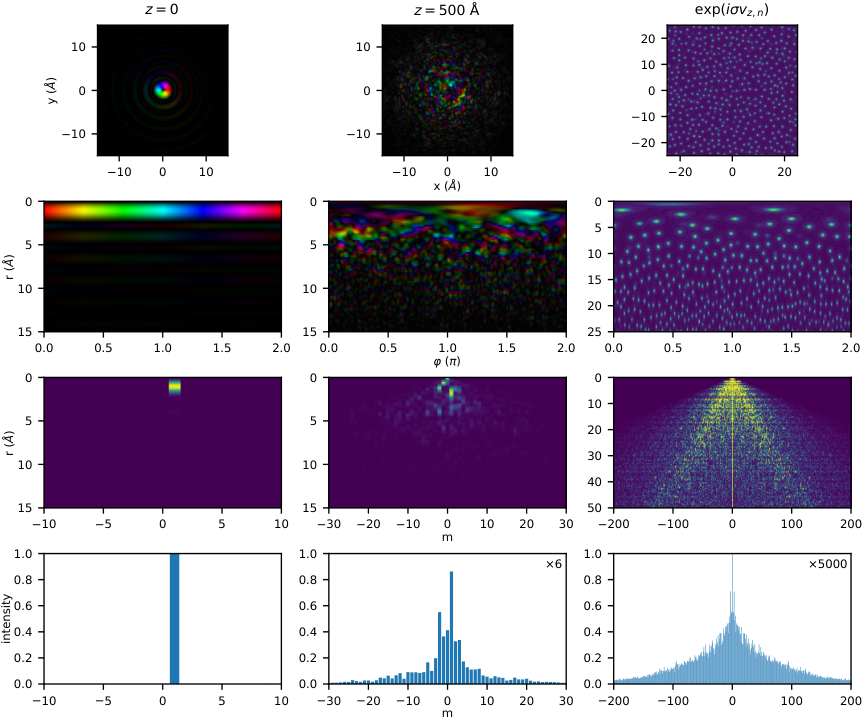
Fig. 3 shows some examples of the data produced by the simulations and during the analysis. In particular, it shows that, as predicted, the redistribution of intensity between different OAM components produced by the scattering potential is approximately symmetric but the resulting wavefunction has a distinctly non-symmetric OAM component distribution around the initial $m=1$ component. Under the given conditions, the $m=1$ component still exhibits the highest intensity, but the components $m\in\{-2,-1,0,2,3\}$ have considerable intensities of the order of $I_{1,n}/2$. Therefore, their sum greatly exceeds $I_{1,n}$. Even higher orders in the range $-20\lesssim m\lesssim 20$ also contribute non-negligibly, further emphasizing the broadness of the $m$ distribution. Interestingly — though not surprisingly — different $m$-components contribute strongly at different radii. In addition, the theoretically predicted linear increase of both the dominant $m\neq 0$ contributions as well as the $m$-spread in the scattering potential is clearly visible.

Fig. 4 shows the dependence of several key quantities on the convergence semi-angle $\alpha$ (which is related to the beam size, see fig. 2) of the incident beam as well as the thickness of the sample for the three simulated systems.

The most striking property is that while the overall features of the graphs are comparable between the three different systems, the numerical values differ greatly. Taking the maximum $\sigma[\hat{L}_{z}]$ as an example, it changes from $\approx 15$ for $\text{Si}{\vphantom{\text{X}}}_{\smash[t]{\text{3}}}\text{N}{\vphantom{\text{X}}}_{\smash[t]{\text{4}}}$ over $\approx 35$ for $\text{Fe}{\vphantom{\text{X}}}_{\smash[t]{\text{0.8}}}\text{B}{\vphantom{\text{X}}}_{\smash[t]{\text{0.2}}}$ to $\approx 65$ for Pt. A similar trend is visible for $\left\langle\hat{L}_{z}\right\rangle$. This phenomenon correlates nicely with the mass density of the three systems. Even though the atom density is comparable for $\text{Si}{\vphantom{\text{X}}}_{\smash[t]{\text{3}}}\text{N}{\vphantom{\text{X}}}_{\smash[t]{\text{4}}}$ and $\text{Fe}{\vphantom{\text{X}}}_{\smash[t]{\text{0.8}}}\text{B}{\vphantom{\text{X}}}_{\smash[t]{\text{0.2}}}$ and is lower for Pt, the mass density increases from $\text{Si}{\vphantom{\text{X}}}_{\smash[t]{\text{3}}}\text{N}{\vphantom{\text{X}}}_{\smash[t]{\text{4}}}$ over $\text{Fe}{\vphantom{\text{X}}}_{\smash[t]{\text{0.8}}}\text{B}{\vphantom{\text{X}}}_{\smash[t]{\text{0.2}}}$ to Pt (see tab. 1), owing to the fact that Pt atoms are much heavier than, e.g. Fe atoms. Since heavier atoms generally scatter more strongly, it is logical that such systems produce stronger OAM deviations.

With respect to the changes of the expectation value $\left\langle\hat{L}_{z}\right\rangle$, fig. 4 shows that the largest net OAM transfers occur for small convergence angles (i.e., large beams) and the smallest deviations occur in the range $5\text{\,}\mathrm{mrad}10\text{\,}\mathrm{mrad}$, especially for small to medium thicknesses. This can be related to the size of the beam as it propagates through the sample. For small $\alpha$, already the incident beam is large compared to interatomic distances and it stays that way all throughout the sample. Thus, large $\delta m$ are possible from the very beginning of the propagation. For large $\alpha$, the diameter of the incident beam is small, but the beam size increases considerably during propagation. Thus, although initially only small $\delta m$ are viable, larger and larger $\delta m$ become dominant as the beam propagates further through the sample. Conversely, a beam with a mid-range $\alpha$ represents a good compromise between small initial size and small growth during propagation, thereby restricting the maximal significant $\delta m$ and, consequently, the variation of $\left\langle\hat{L}_{z}\right\rangle$. A similar result was also found for classical EMCD (where vortex beams are generated during inelastic scattering and subsequently analyzed interferometrically) in crystalline samples [M_v67_i_p60].

For $\sigma[\hat{L}_{z}]$ — i.e. the OAM uncertainty or, equivalently, the spread of the $m$ distribution —, the picture is very similar. Small $\alpha$ lead to a very large increase in $\sigma$ with thickness. For medium $\alpha$ in the range of $7\text{\,}\mathrm{mrad}13\text{\,}\mathrm{mrad}$, $\sigma$ is smallest, while it increases again for large $\alpha$.

Interestingly, the $\alpha$-dependence is different for the $m=1$ intensity, which gives an indication “how much” of the original, incident beam structure actually is present at a given thickness. Fig. 4 shows that $I_{1,n}$ obviously decreases with thickness, but is mostly independent of $\alpha$. In other words: even though the net OAM and the $m$ distribution depend strongly on the beam size through the convergence angle and although there is complex multiple scattering going on back and forth between different $m$ components at different radii (as visible from fig. 3), the overall intensity of the $m=1$ component seems to be fairly predictable.

To investigate the intensity of different $m$ components as well as the expectation value in more detail, fig. 5 shows graphs of the intensity of $m=1$ as well as the adjacent components $m=0,2$ and $\left\langle\hat{L}_{z}\right\rangle$ for different convergence semi-angles $\alpha$ as a function of thickness. The adjacent components were selected because for applications that depend on the fact that the beam is in an $m=1$ eigenstate (such as, e.g. EMCD), typically close-lying other components are more difficult to separate than far-removed ones. As an example, an $m=100$ vortex would have practically zero intensity everywhere where an $m=1$ vortex is strong, thus making it easy to separate and block, e.g., by an aperture.

As before, the overall behavior of the curves is roughly similar for the $m$ components of all three studied systems, except for the scale of the thickness-dependence, which, again, is more dramatic for heavier specimens. Nevertheless, there are several noteworthy aspects visible in the graphs. In the first several Ångström, the decay of the $m=1$ intensity as well as the increase of the adjacent components is practically linear. This is to be expected as for a dominant $m=1$ component, the transitions $1\mapsto 0$ and $1\mapsto 2$ will be much more probable than the scattering $0\mapsto 1$, $0\mapsto-1$, etc. However, after several Ångström, all depicted components start to deviate from their linear behavior. The $m=1$ intensity decrease starts to slow down as soon as it reaches $\approx$70\text{\,}\mathrm{\%}$$ of the initial intensity, while the $m=0,2$ intensities become almost constant somewhere in the range of $10\text{\,}\mathrm{\%}20\text{\,}\mathrm{\%}$. As the thickness increases, the $m=0,2$ components seem to asymptotically tend towards a similar behavior as the $m=1$ component, as is visible for Pt at $\alpha=$25\text{\,}\mathrm{mrad}$$ and — to some degree — already at $\alpha=$10\text{\,}\mathrm{mrad}$$. Note that in all cases, the variation over several runs clearly indicates that the results are statistically significant, although the margin of error naturally is larger for larger mass density.

As already shown in fig. 4, the decrease in $m=1$ intensity does not depend strongly on the convergence angle. However, the the increase of the adjacent components is influenced by the convergence angle. At the same time, the statistical uncertainty increases substantially for increasing convergence angles (i.e., smaller beam waists). This can be attributed to the fact that for sufficiently small beams (i.e., smaller than the inter-atomic distance), the propagation behavior is crucially dependent on the (random) relative position of the beam with respect to close-by atoms, whereas for large beams, the effect is averaged over many atoms.

Another interesting result can be found in the behavior and statistical variation of the expectation value $\left\langle\hat{L}_{z}\right\rangle$. For $\text{Si}{\vphantom{\text{X}}}_{\smash[t]{\text{3}}}\text{N}{\vphantom{\text{X}}}_{\smash[t]{\text{4}}}$, the deviation from $\hbar$ is marginal and fairly well contained in the statistical error. For heavier systems, the deviation from $\hbar$ become much stronger — with a general trend towards decreasing $\left\langle\hat{L}_{z}\right\rangle$ —, but also the statistical variation between different simulations increases, up to the point that for Pt at $\alpha=$25\text{\,}\mathrm{mrad}$$, the deviation from $\hbar$ is no longer significant.

Whether the results presented here are encouraging or discouraging depends on the application at hand, the system under investigation, and the chosen experimental parameters.

If pure vortex beams are required, low mass-densities as in the case of $\text{Si}{\vphantom{\text{X}}}_{\smash[t]{\text{3}}}\text{N}{\vphantom{\text{X}}}_{\smash[t]{\text{4}}}$ and low thicknesses are definitely preferable in order to retain a high intensity in the $m$-component of the incident beam as well as little variation for different atom configurations. This also implies that holographic phase masks fabricated on a thick $\text{Si}{\vphantom{\text{X}}}_{\smash[t]{\text{3}}}\text{N}{\vphantom{\text{X}}}_{\smash[t]{\text{4}}}$ membrane can be subject to a considerable loss of mode purity.

If a high net OAM transfer is sought (e.g., in the case of nanoparticle manipulation), high mass-densities as in the case of Pt as well as thick samples and medium convergence angles should be used. This ensures a large OAM transfer while retaining acceptable statistical variations for different atom positions.

It should be noted that real sample densities and scattering strengths may differ from the ones presented here, e.g. due to the use of different materials. In addition, the sample density is influenced by deposition and preparation parameters. However, the materials presented in this work span from fairly low to quite high mass densities and scattering strengths, thus giving a general insight into how arbitrary samples will behave.

All the simulations presented in this work were performed under ideal conditions, including no incoherent source size broadening (ISSB), no atom movement, and no lens aberrations. Both ISSB and atom movement would lead to an effectively different relative position between the beam and the atoms for each electron in the beam. This is conceptionally equivalent to the averaging over several random atom configuration as done in this study. Lens aberrations generally lead to a coherent broadening of the beam compared to the ideal case. While in such a situation the details of the amplitude and phase of the beam change, the overall results should be the same as those presented here when considering the appropriate beam size (see fig. 2).

In this work, we presented extensive simulations of the propagation of electron vortex beams through amorphous materials. To that end, we have rewritten the multislice approach into cylindrical coordinates to get some theoretical insight into the vortex propagation, such as the beam-size dependence of the redistribution of intensity between different $m$ components and the possibility of net OAM transfer despite the fact that the probabilities for transferring $\pm\delta m\cdot\hbar$ are (approximately) equal. In addition, we have also described the influence of the point group symmetry on the vortex propagation.

The numerical simulations were performed for the three amorphous model systems $\text{Si}{\vphantom{\text{X}}}_{\smash[t]{\text{3}}}\text{N}{\vphantom{\text{X}}}_{\smash[t]{\text{4}}}$, $\text{Fe}{\vphantom{\text{X}}}_{\smash[t]{\text{0.8}}}\text{B}{\vphantom{\text{X}}}_{\smash[t]{\text{0.2}}}$, and Pt for a wide range of convergence semi-angles and thicknesses. Besides corroborating the theoretical results, the numerical data allowed us to quantify the net OAM transfer, the spread of vortex components that is related to the uncertainty principle and, thus, the purity of a vortex state, as well as the intensity behavior of the most important vortex components. The results showed that in order to retain high purity upon propagation, low-mass-density samples with small thickness should be chosen, while large net OAM transfers can best be achieved in heavy, thick samples. In both cases, intermediate convergence semi-angles around $\alpha\sim$10\text{\,}\mathrm{mrad}$$ proved beneficial.

The results presented in this work will allow theoreticians and experimentalists alike to choose the material for their studies with electron vortices more efficiently. Although this work does not completely replace full simulations for future studies, it does give some general insight into the propagation behavior of EVBs and makes predictions for a large range of systems and experimental parameters. As such, it promises to contribute to future enhancements not only of the fabrication but also of the applications of electron vortex beams.

T.S. acknowledges financial support by the Austrian Academy of Science (ÖAW) for the DOC scholarship and the “Hochschuljubiläumsstiftung der Stadt Wien” (project H-294689/2016).

[bibexport]