Desingularization of matrix equations employing hypersingular integrals in boundary element methods using double nodes Journal: Engineering Analysis with Boundary Elements (Accepted June 11, 2019)
Abstract
In boundary element methods, using double nodes at corners is a useful approach to uniquely define the normal direction of boundary elements. However, matrix equations constructed by conventional boundary integral equations (CBIEs) become singular under certain combinations of double node boundary conditions. In this paper, we analyze the singular conditions of the CBIE formulation for cases where the boundary conditions at the double node are imposed by combinations of Dirichlet, Neumann, Robin, and interface conditions. To address this singularity, we propose the use of hypersingular integral equations (HBIEs) for wave propagation problems that obey the Helmholtz equation. To demonstrate the applicability of HBIE, we compare three types of simultaneous equations: (i) CBIE, (ii) partial-HBIE where the HBIE is only applied to the double nodes at corners while the CBIE is applied to the other nodes, and (iii) full-HBIE where the HBIE is applied to all nodes. Based on our numerical results, we observe the following results. The singularity of the matrix equations for problems with any combination of boundary conditions can be resolved by both full-HBIEs and partial-HBIEs, and the partial-HBIE exhibits better accuracy than the full-HBIE. Furthermore, the computational cost of partial-HBIEs is smaller than that of full-HBIEs.
Keywords:
Boundary element method, Hypersingular integral, Helmholtz equation, Double node, Corner, Boundary condition, Regularization of coefficient matrix, Rank deficiency1 Introduction
The boundary element method (BEM), the finite difference method (FDM), and the finite element method (FEM) have been commonly used to solve boundary value problems. In the BEM, a set of simultaneous equations for determining unknown variables at nodes on the boundary is constructed in discretized boundary integral equations. The variables in simultaneous equations are nodal field values and normal derivatives only on individual boundary nodes, whereas the variables in the FDM or FEM are field values at domain nodes which are placed in the entire domain enclosed by the boundary. Therefore, the number of variables in the BEM is much smaller than that in the FDM or FEM, which is one of the advantages of BEM. Furthermore, the BEM can be easily applied to external problems, such as wave scattering problems, since it does not require the placement of nodes in a domain spreading to infinity and it does not require any other boundary conditions to represent radiation at a boundary enclosing the domain considered.
In most boundary problems, the field values, , along the boundary are continuous; however, the normal derivatives, , are discontinuous at corners since the normal directions at any corner point are different. By using a linear element or higher-order elements, the boundary elements share the nodes at both ends of the element with adjacent boundary elements. In this case, the normal direction, , at the corner node cannot be defined uniquely since the single node at any corner belongs to two boundary elements with different normal directions.
There are two approaches to addressing the definition problem of the normal direction. The first approach involves the use of non-conforming elements, which are also called discontinuous elements. In the non-conforming element, collocation nodes that represent and do not coincide with geometric nodes, but they do so in the conforming element. The non-conforming element has been applied to several problems; e.g., elastostatic problems Manolis:1986, Parreira:1988, Olukoko:1993, Blazquez:1994, Huesmann:1994, Paris:1995, Blazquez:1998, fluid flow problems Patterson:1982, Dyka:1989, and acoustic problems Silva:1993. Although the accuracy between the non-conforming element and the conforming element were compared by Manolis and Banerjee Manolis:1986, and Parreira Parreira:1988, they arrived at different conclusions.
The second approach includes a double node technique Brebbia:1984:Sec_5_2 or a multiple node technique for three-dimensional problems. In the double node technique, two normal derivatives, and , and a field, , are defined at the corner node, where and denote the directions normal to the two boundary elements connected to the corner node. However, a set of simultaneous equations, called a matrix equation, becomes singular under certain boundary conditions; i.e., the rank of the matrix equation is reduced since some node equations are redundant. Further details will be presented in Sec. 2.
To address the rank reduction problem caused by the double nodes, there are two categories of approaches. The first category involves the use of a local relation for each double node Walker:1989, Yan:1994, Kassab:1994, Gao:2000. By using a Taylor expansion around the corner node, this relation is described as a linear combination of the two normal derivatives and the field values at neighbor nodes of the corner node. The local relation is replaced by one of the redundant equations that reduces the rank; therefore, the matrix equation still includes a square matrix. In the second category, extra node equations are employed Mitra:1987, Mitra:1993, Subia:1995, Deng:2013, Zheng:2018. Mitra and Ingber Mitra:1987 proposed a technique for replacing one of the redundant equations in each corner by an extra node equation with respect to an extra collocation node placed outside the domain considered. Following this study, the authors mentioned that “external collocation yields a coefficient matrix with a large number” Mitra:1993, and they improved the method using the extra node equations so that the location of the extra node on the boundary elements connects to the double node Mitra:1993, Subia:1995. Subia, Ingber, and Mitra demonstrated that there are no significant differences in accuracy between the method of the extra node equation and the non-conforming method Subia:1995. The method that uses the extra node equations was extended to the problems of interface boundaries at which two or more domains are connected Deng:2013, Zheng:2018. Using these methods, the number of variables is not increased since the field at the extra node is known. Therefore, the coefficient matrix is the square matrix, which is similar to the matrix of the first category. If we simply add the local relations shown in the first category or the extra node equations in the second category instead of replacing them, the number of equations becomes larger than the number of variables, which is referred to as an overdetermined problem. We can solve this equation by using least-square methods, but the computational time required to solve this equation is much greater than solving the general simultaneous equation; therefore, the replacements are generally applied. The replacement of the equation should be performed individually while examining the types of boundary conditions at the corner. The individual examination increases the complexity of the programming of widely applicable BEM codes that include many types of boundary conditions.
In addition to the corner node problems, there are rank deficient or large condition number problems. We focus on two problems related to hypersingular boundary integral equations. The first is a non-uniqueness or a spurious solution problem in an external field for a wave scattering problem that obeys the Helmholtz equation, in which the domain considered is outside of the boundary enclosing a scatterer. In this situation, spurious solutions can be obtained at the eigenfrequency of the scatterer. To resolve this problem, two major approaches were proposed. Schenck employed equations related to additional nodes in the scatterer region and the method is called ‘Combined Helmholtz Integral Equation Formulation (CHIEF)’ Schenck:1968. Chen et al. IL_Chen:2001 applied the additional node equations to interior problems in which additional points are placed outside of the boundary. These methods are similar to the extra node equation methods for the corner problems shown in the previous paragraph; however, they require a solver based on the least-square method since the set of simultaneous equations becomes an overdetermined equation. The other approach is referred to as the Burton-Miller method Burton-Miller:1971, Benthien:1997, Diwan:2013, Langrenne:2015. Burton and Miller Burton-Miller:1971 represented a boundary integral equation (BIE) for each node using a linear combination of two types of BIE called a conventional BIE (CBIE) and a hypersingular BIE (HBIE). In the CBIE, the field at the field point is denoted by integrals over the boundary on which sources are distributed. The HBIE is obtained by taking a gradient of the CBIE. The singularity of the integral in the HBIE is stronger than that of the CBIE; therefore, it is called a hypersingular integral. Bentihien and Schenck Benthien:1997 reviewed the non-uniqueness problem with comparisons of other methods, including the CHIEF and Burton-Miller methods.
The other rank deficient problem is found at a degenerate boundary which appears either at a crack in an elastostatic problem Portela:1992, JT_Chen:1994, Chyuan:2003, Lu:2010 or at both surfaces of a thin metal with zero-thickness in an electromagnetic problem Chyuan:2003. To resolve these problems, the CBIEs are applied to one side of the crack or the thin metal, and the HBIEs are applied to the other side. These methods are referred to as dual-BEM.
As shown in the previous two paragraphs, the use of HBIEs is effective for resolving rank deficient problems. In this paper, we will demonstrate that the corner singular problem for wave propagation problems can be solved by only using node equations based on HBIEs. In addition, to suppress the rank deficiency caused by the corners, we do not need to use HBIEs for every node. We will also illustrate that only the replacement of the node equations related to the corner node by HBIEs is sufficient, which is similar to the aforementioned dual-BEM.
In the application of HBIEs, the regularization of hypersingularity is a key issue. The authors developed an analytical regularization of the two-dimensional Helmholtz equation Tomioka:2010; the other regularization methods are also found in the references of that study. In the regularization of HBIEs, we include the relations between two normal derivatives at the double nodes, similar to the local relation methods described above. Therefore, the method by HBIE can be considered an extension that uses the local relation. However, the contributions to the double node from all the nodes are considered in the method by HBIE; whereas the local relation method represents the relations between local nodal quantities only.
The method proposed in this paper to overcome the corner problem caused by the double nodes does not require local relations at corners, extra node equations, or least-square methods. Our method can also be applied to any kind of boundary conditions of boundary elements that include corner nodes. In addition, the proposed method can also be applied to interface boundary conditions. From these characteristics, no additional effort is required in prepossessing to prepare the input data for solving the boundary value problem.
The outline of this paper is as follows. In Sec. 2, we demonstrate why the rank of the coefficient matrix of the CBIE is reduced in the case where the double node is employed. We also demonstrate the condition that results in rank deficiency based on the nature of the discretized node equations. In Sec. 3, we illustrate why the HBIE does not cause a rank deficiency. The numerical results and discussions for simple waveguide problems are presented in Sec. 4 to demonstrate that the HBIE is applicable to any combination of boundary conditions. The advantages of the partial-HBIE method in which the HBIE is applied to only the double nodes and the CBIE is applied to other nodes are also shown. Finally, the summary is presented in Sec. 5.
2 Rank deficiency problem in CBIEs
To illustrate rank deficient conditions for a set of discretized node equations of CBIEs, the discretization using linear elements is first shown; the double node technique that defines two sub-nodes for a double node are then shown; and lastly, the rank deficiency conditions are discussed based on comparisons between two equations for the two sub-nodes.
2.1 Discretization of CBIEs
A complex-valued time harmonic scalar wave satisfies the following Helmholtz equation with an assumed time factor , where is an imaginary unit and is the angular frequency:
| (1) |
where indicates the wave number, which is a ratio of to the wave velocity, and represents the spatial domain considered. A fundamental solution , which represents the contribution to a field point from a unit source placed at a source point in free space satisfies
| (2) |
where the differential operator operates only on , but not on . This equation can be solved analytically. In two-dimensional problems, the outward propagating wave that obeys Eq. (2) is
| (3) |
where the function is a second kind 0-th order Hankel function.
Using Green’s second identity and some integral operations for Eqs. (1) and (2), we obtain the conventional boundary integral equation (CBIE),
where denotes a boundary surrounding , is the position of the source point on the boundary, is the position of the field point, is the outward-pointing normal unit vector; the contour integral is evaluated as a Cauchy principal value, and is the result of the following evaluation of Dirac’s delta function:
| (5) |
The coefficient depends on the shape of the boundary at the field point . Because of the nature of Dirac’s delta function, when is located inside and outside the domain, evaluates to 1 and 0, respectively. In the case where is located on , is equal to the ratio of the interior angle to the whole angle; e.g., for 2-dimensional problems. In addition, when we introduce a fundamental solution to a Laplace equation, , which satisfies
| (6) |
the coefficient can be expressed by a boundary integral:
| (7) |
which is called an equipotential condition Brebbia:1980.
When is located on and the boundary is partitioned into a number of boundary elements, Eq. (2.1) can be written as a node equation for the node as a discrete algebraic expression:
| (8) |
where both the superscripts and the subscripts and denote the node numbers and not the element numbers; denotes a set of the node numbers, which includes members; denotes the Kronecker’s delta; and . The factors and are results of boundary integrals in Eq. (2.1) as shown below.
In Eq. (8), there are two variables, and , at . One of them is specified by a boundary condition as a boundary value which is denoted by , and the other is an unknown variable denoted ; therefore, the number of variables is equal to that of the nodes, . Since the node can be placed at every boundary node, we can obtain equations of Eq. (8) as
| (9) |
where both and are either or when simple boundary conditions are specified. The matrix composed of is called a coefficient matrix in the following discussions.
The coefficient represents the contribution to from the nodal quantity at the node , and represents the contribution to from . These coefficients are evaluated by boundary integrals, which depend on a method that interpolates and along the boundary element. To examine the nature of and , we present evaluations using a shape function to interpolate them. Let us consider the discretization of the boundary integral of . By denoting the -th boundary element as and a local node number as , on is represented by a linear combination of shape functions and at the boundary nodes:
| (10) |
where denotes the number of nodes in a boundary element; e.g., for the linear element, for the second-order element. A global node number can be mapped from the local node numbers by a permutation matrix :
| (11) |
where has the value 1 if and are associated, and 0 otherwise. Although the notation of is used here, it provides a symbolic meaning, and it is treated as a mapping function such as in actual coding to avoid summation procedures with respect to . By using these definitions, the boundary integral is discretized as
| (12) |
where and are defined as
| (13) | ||||
| (14) |
The integral on the right-hand side in Eq. (13) is evaluated by a numerical integral such as Gauss quadrature or by an analytical integral in the case of , which is called a singular integral. Similarly, the other integral in Eq. (2.1) is evaluated as
| (15) | ||||
| (16) | ||||
| (17) |
where , which is not the derivative at ; i.e., does not depend on .
To discuss the rank of the matrix equation shown in Eq. (9), the dependencies of both and on which is the normal unit vector at are important. First, is independent of since Eqs. (13) and (14) do not include regardless of or . In contrast, the case of is different from that of . Although in Eqs. (16) and (17) looks independent of even when is expressed using , there is an exception at in which becomes . The dependency of this exceptional case is presented in the next section.

2.2 Double node technique
In the node equation for node shown in Eq. (8), both and are values of the nodes, which are located at the two ends of the boundary element in the case of the linear element. When the node is located at a corner, the normal derivative of the linear element cannot be defined uniquely since the node belongs to two elements with different normal directions. Using a double node technique is one of the solutions.
Figure 1 illustrates a configuration of a double node. The node is represented by two sub-nodes at the same position; . The node at is connected to both and a zero-sized element between and , and vice versa. The normal direction of the sub-nodes and can be determined from the directions normal to and , respectively; therefore, the direction of the derivatives of and can be defined individually. Since the integral along the zero-sized element is identically zero regardless of the normal direction, we do not need to define the normal direction for the zero-sized element. Although the node does not belong to , contributions of and , which are evaluated by analytical integrals as singular integrals for accurate evaluation, are similar to and .
Both and are defined at each sub-node in the same way as ordinary nodes, and the boundary condition is imposed for each sub-node. Either or is unnecessary since ; however, the same representation as the ordinary nodes simplifies the programming effort. In this case, the number of unknown variables increases by the number of double nodes, which equals the number of corners. Since one double node is replaced by the two sub-nodes and for each corner, the number of node equations is also increased by the number of corners. Consequently, a set of CBIEs can be expressed by a matrix equation with a square coefficient matrix even when we apply double nodes.
Since the integral along the zero-sized elements is zero, the right-hand sides of Eq. (7) for and are the same. Therefore, the coefficients and must have the same value:
| (18) |
In the case of linear elements, the singular integral of for the corners () becomes zero since the for or is perpendicular to for or :
| (19) |
Therefore, summarizing the discussions in the last paragraph in Sec. 2.1 and this result, we obtain the relations for the sub-nodes as
| (20) | ||||||
| (21) |
2.3 Rank deficiency conditions in CBIEs
By using the double node technique, the boundary nodes including sub-nodes are defined at the ends of boundary elements, and the boundary conditions are defined at each node. In problems with a single medium, there are three common types of boundary conditions; Dirichlet condition, Neumann condition, and Robin condition. These conditions are given, respectively, as
| (22) | ||||||
| (23) | ||||||
| (24) |
where the over-bars denote values imposed by the boundary conditions, and are the given constants determined by the problem considered, and the sets of the node numbers with corresponding boundary conditions are denoted by , , and , respectively.
When we consider a multi-media problem, there exists a condition at the interface between the media. The interface condition is expressed by two continuous conditions for and . The continuous conditions are given as
| (25) |
where media numbers are denoted by (1) and (2); the nodes and are located at the same positions; is determined by media constants of and ; and denotes the set of nodes with interface conditions.
In this section, we first present three simple examples when two sub-nodes of a double node at a corner point belong to or , and discuss why the rank deficient problem arises. Then, the case in which the sub-nodes belong to or are presented.
The combinations of the boundary conditions where the two sub-nodes, and , belong to or are classified into the following three cases:
- 1.
both include the Dirichlet conditions: and ,
- 2.
both include the Neumann conditions: and ,
- 3.
one includes the Dirichlet condition and the other includes the Neumann condition:
and , or and .
2.3.1 Case of two Dirichlet conditions
Under these conditions ( and ), the sub-node equations of Eq. (8) for and can be arranged so that the terms including known values are moved to the right-hand side and the terms related to and are moved out from the summation as
| (26) | ||||
| (27) |
where , i.e., all nodes, and denotes a set of all node numbers except and ; and the detailed descriptions of the third terms on the left-hand sides and the right-hand sides are written as
| (28) | ||||
| (29) |
Comparing the coefficients of the terms on the left-hand side of the two sub-node equations shown in Eqs. (26) and (27), we can evaluate whether the rank of the coefficient matrix is reduced or not. From Eqs. (20) and (21), the contributions and () to the node are the same. The coefficients and share the same value from Eq. (18); however, the multiplied terms, , are different since is also multiplied by the Kronecker’s delta in Eq. (8). Therefore, we can examine rank reduction by examining which terms simply include the Kronecker’s delta. The Kronecker’s delta is not found in the first and the second terms on the left-hand sides in Eqs. (26) and (27). For the third terms, node does not include and ; therefore, the and are not included. They only appear in the right-hand sides, which are not related to rank reduction. Therefore, the left-hand sides of the two equations are identical, and the rank is always reduced by these two sub-node equations; i.e., the coefficient matrix becomes a singular matrix.
2.3.2 Case of two Neumann conditions
As in the previous sub-section, two sub-node equations of Eq. (8) in the case of and can be arranged as
| (30) | ||||
| (31) |
Although the definitions of and are different from Eqs. (28) and (29), the third terms of Eqs. (30) and (31) are identical since they do not include the Kronecker’s delta. In contrast, the first and second terms are different. By applying Eqs. (18) and (19), the coefficients associated with and in Eq. (30) are and 0, respectively; while those in Eq. (31) are 0 and , respectively. Therefore, the rank of the matrix that includes the sub-node equations is not reduced in the case of and . In addition, the right-hand sides are the same since they do not include the Kronecker’s delta. This means that the results of these two sub-node equations involve the relation .
2.3.3 Case of coupled Dirichlet and Neumann conditions
In the case of and , two sub-node equations are
| (32) | ||||
| (33) |
Since the second terms on the left-hand sides of the above equations are different, the rank of the coefficient matrix is not reduced in the case of and .
2.3.4 Case of Robin condition
We consider the case in which the Robin conditions are imposed on at least one of the two sub-nodes. Eliminating from Eq. (8) using Eq. (24), and arranging the equation, we obtain:
| (34) |
When , the term with the factor for unknown remains in the third terms of the left-hand side. This satisfies the condition described at the end of Sec. 2.3.3, which ensures that the equations of the two sub-nodes are independent and not identical. It does not depend on the type of boundary condition of the node .
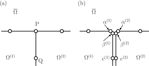

2.3.5 Case of interface condition
Figure 2 illustrates a configuration around a double node where two domains are in contact. The corner node labeled P is represented by the four sub-nodes at the corner; two sub-nodes labeled and do not belong to the interface boundary, and the other two sub-nodes labeled and belong to the interface boundary. There are eight quantities related to these four sub-nodes. Of the eight quantities, two quantities at the sub-nodes and are considered ordinary boundary conditions, and two variables at and can be eliminated by the interface conditions shown in Eq. (25), which, for and , are rewritten as
| (35) |
where the double suffixes, such as , are denoted by for simplicity. Consequently, there are four unknown variables and four equations with respect to the double node when we apply these conditions before constructing the simultaneous equations.
As mentioned in the previous sub-sections, the coefficients unrelated to the sub-nodes do not affect rank reduction; therefore, we only consider the nature of the sub-matrix composed of the coefficients for the four unknown variables.
In the case of and , the given values are and , and the unknown variables are , , , , , and . The independent variables are reduced by using Eq. (35) such as . The terms associated with these independent variables in the individual sub-node equations for , , , and , are written as
By applying Eqs. (18), (19) and (20) to the sub-matrix to eliminate coefficients with the subscript and , the sub-matrix is rewritten as
Furthermore, by applying elementary matrix operations, the sub-matrix is transformed to
where the second row is the result of replacement with the difference between the first and the second row of the matrix in Eq. (2.3.5), and the fourth row is obtained by similar operations. The non-zero components in both the second and the fourth row are only found in the fourth column; therefore, the rank of this sub-matrix is reduced by one.
2.3.6 Case of internal interface condition
In the case where the node is located at a corner of two interface boundary elements as shown in Fig. 3(a), there are four sub-nodes at the corner node. After applying Eqs. (18), (19) and (20), and eliminating the quantities related to and , the terms related to the sub-nodes in the four sub-node equations are expressed as
By applying the elementary matrix operations to the coefficient matrix, the matrix is transformed to
We can understand that the rank of this matrix is reduced by one since the determinant of a 2x2 sub-matrix composed of non-zero elements in the second and the fourth row in the above sub-matrix is zero. When we increase the number of the domains as shown in Fig. 3(b), we can illustrate the singularity, although the details are not shown here. Therefore, the sub-node equations become singular when the node is located at an intersection of the interface boundaries which partitions the original single domain into two or more domains.
2.4 Summary of rank deficiency conditions for CBIEs
In this section, we analyze the rank deficiency conditions for the sub-node equations of a double node for CBIEs. The rank of the coefficient matrix is reduced in the following cases:
- 1.
both sub-nodes of a double node are imposed by Dirichlet conditions,
- 2.
sub-nodes are located at an intersection of an interface boundary element and two boundary elements imposed by Dirichlet conditions,
- 3.
sub-nodes are located at intersections of interface boundary elements with different normal directions and they do not belong to any boundary with ordinary boundary conditions.
The original sub-node equations or the sub-matrix associated with the sub-nodes for these cases include a pair of Eqs. (26) and (27) for the first case, Eq. (2.3.5) for the second case, and Eq. (2.3.6) for the last case. These equations have common characteristics; all the equations include and (or and for the interface boundary) as the unknown variables. The coefficients associated with these unknowns are (), which possess the characteristics shown in Eq. (20). The terms with and are canceled because of this characteristic during the transformations of the equations, and the ranks have been reduced.
If the coefficients did not satisfy Eq. (20); in other words, if they included information on , these singularities could be avoided.
3 Regularization of coefficient matrix using HBIEs
As described in Sec. 2.4, the reason for a rank deficient matrix in CBIE is the coefficients do not carry information concerning the normal direction of the node . To provide this information, we employ a hypersingular boundary integral equation (HBIE). The HBIE can be derived by taking a gradient of the CBIE shown in Eq. (2.1) with respect to :
| (80) |
where denotes the gradient with respect to . The gradient, , has a stronger singularity than the CBIE, and this is known as hypersingularity. However, the integral of the hypersingular function can be regularized. In this study, we employ the regularization for the Helmholtz equation which uses the fundamental solution of Laplace’s equation Tomioka:2010.
3.1 Regularized gradient field
In this section, after presenting a regularization of the gradient at according to the method shown in Ref. Tomioka:2010, a discretized form of the normal derivative, , is derived.
The gradient is expressed by a 2x2 dyadic tensor and a vector as
| (81) |
The second term can be evaluated by two types of boundary integrals as
| (82) |
where is associated to the boundary integral along the boundary elements that include the node and (Fig. 1); whereas corresponds to integrals of the boundary elements not including the node . Similar to the factor in CBIEs, the singular integral included in Eq. (3) contributes to on the left-hand side of Eq. (81) and . The components of , and are written as
| (83) | ||||
| (84) | ||||
| (87) |
where denotes the fundamental solution to the Laplace equation that satisfies Eq. (6), is its normal derivative with respect to at ; and , , and are the tangential unit vectors along , the azimuth angle of from , and the length of , respectively.
Similar to CBIEs, the non-singular integral in Eq. (84) is expressed by the shape function as
| (88) | ||||
| (89) | ||||
| (90) |
which are evaluated using numerical integrals. By using the permutation matrix, the second term on the left-hand side in Eq. (82) is denoted by a form of linear combinations as
| (91) |
The two singular integrals on the right-hand side of Eq. (3.1) can be analytically obtained by using Taylor series expansions around for the two second-order derivatives. The first term on the right-hand side of Eq. (82) is also expressed as linear combinations with respect to the nodes neighboring the sub-nodes and as
| (92) |
By defining
| (93) |
the vector is expressed as the following form with a linear combination:
| (94) |
By substituting this equation into Eq. (81) and by multiplying both sides by , the gradient field at is expressed as
| (95) |
3.2 Rank deficiency conditions in HBIEs
Let us consider the relations of and when is a double node; i.e., . If both and at all nodes are determined as known values, the gradient in Eq. (95) must be expressed uniquely. Since the dyadic tensor on the right-hand side of Eq. (95) is determined by a geometric configuration of the boundary elements connected to as shown in Eq. (3.1), is satisfied. Therefore, to uniquely determine the gradient, i.e., , the coefficient vectors for and must be the same. Strictly speaking, there is an exception in for . In this case, the condition is permitted when is satisfied since . Therefore,
| (96) | ||||||
| (97) | ||||||
| (98) |
Since , by taking an inner product of to Eq. (95), the discretized equation for the HBIE is obtained as
| (99) |
where
| (100) | ||||
| (101) |
When , we can derive the following conditions using Eqs. (97) and (98):
| (102) | ||||||
| (103) |
These relations mean that the two sub-node equations of Eq. (99) for and are different. Even in the case of , the two sub-node equations are also different since the coefficients for of the two equations are always different because of Eq. (96) and the coefficients for are always different because of the nature of .
The aforementioned difference in the two equations is not a sufficient condition to not reduce the rank since we have not proved that the determinant of the sub-matrix associated with the sub-nodes is not equal to zero for any problem. However, the HBIE is highly applicable to the problem in which the node equations constructed by the CBIE become singular.


4 Numerical results and discussions
To demonstrate the validity of the method in regularizing the coefficient matrix using HBIEs, we analyzed simple models as shown in Fig. 4. The actual models correspond to electromagnetic wave propagation problems in a waveguide where the wall parallel to the propagation direction is made of metal. When we consider as the -component of the electric field, at the side-walls of the waveguide since the component of the electric field parallel to the metal is zero. In the case of model-(A), the metal walls are located at , which is called the TE10 mode for a waveguide with rectangular cross-section and width . In the case of model-(B), virtual walls with are located at , which are equivalent to the placement of physical metal walls with at , which is called the TE20 mode. These incident conditions are given as functions of as
| (104) | ||||||
| (105) | ||||||
| (106) | ||||||
In these modes, a propagation field to -directions are proportional to , respectively, where
| (107) |
By using this characteristic, the incident boundary condition on can be rewritten as a Robin condition:
| (108) |
On the boundary at , we analyzed the following three conditions for termination:
| (a) | Short: | (), | |
|---|---|---|---|
| (b) | Open: | (), | |
| (c) | Non-reflective: | (), |
where denotes the reflection coefficient of the electric field on ; and the non-reflective condition in (c) is equivalent to the incident condition with in Eq. (108). Among the above three, termination-(a) (short type) has two double nodes at , where both sub-nodes have two Dirichlet conditions; therefore, the rank of the coefficient matrix of CBIEs will be reduced as mentioned in Sec. 2.3.1. The exact solutions to these models are given by
| (109) | ||||||
| (110) |
To simplify, we used , , , and ; under this condition, for the cases (a) and (b), and for the case (c), and . As examples of , the real part of for the models (A-b) and (B-b) are shown in Fig. 5.
We analyzed three types of the following simultaneous equations:
- (i)
CBIE: BIEs for all nodes including sub-nodes are obtained from the CBIE,
- (ii)
partial-HBIE: BIEs for only sub-nodes related to double nodes are obtained from the HBIE, and BIEs for the other nodes are obtained from the CBIE.
- (iii)
full-HBIE: BIEs for all nodes including sub-nodes are obtained from the HBIE,
To solve the complex-valued simultaneous equations, we employed two subroutines based on an LU decomposition provided in Lapack Lapack, in which the subroutine names are ‘zgetrf’ and ‘zgetrs.’ After determining both and at all boundary nodes by solving the simultaneous equations, the internal field can be evaluated by
| (111) |
which is derived from the discretized CBIE shown in Eq. (2.1). This process is the same for all types of simultaneous equations.
Figure 6 presents the distributions of errors based on the three types of simultaneous equations (i), (ii), and (iii) for the model-(A-b) and model-(B-b). In these models with termination-(b) (open type), the coefficient matrices, even in the case of the CBIE shown in Fig. 6(i), are not singular as mentioned in Sec. 2.4.
Based on the comparison between the sub-figures (A-b-i) and (A-b-iii) or between (B-b-i) and (B-b-iii) in Fig. 6, we can observe that the error of the full-HBIE is several times larger than that the CBIE. This difference can be explained by two reasons. The first reason is the difference in singularity to evaluate the coefficients. The coefficients and in the HBIE are evaluated from and with a multiplication of dyadic as shown in Eqs. (100) and (101), respectively. The vectors and are evaluated by the boundary integral shown in Eqs. (88), (89) and (90). Their integrands include the first or second order derivatives of the fundamental solution. The strongest singularity in the HBIE is , while the strongest singularity in the CBIE is . This error emerges significantly in the contributions between two nodes with short distances. The second reason is the multiplication by . In the worst case, the errors of and are multiplied by the maximum norm, , and the errors of and , respectively. This amplification affects all coefficients regardless of the distances between nodes. According to Ref. Tomioka:2010, in the case of and .
In contrast, the error in the case of the partial-HBIE shown in Fig. 6(A-b-ii) is similar to the case of the CBIE in (A-b-i); and the relation between (B-b-ii) and (B-b-i) is also similar. The number of unknowns in the analyses presented in Fig. 6 was 164 including four double nodes; i.e., the number of HBIEs was only 8 and the number of CBIEs was 156 in the partial-HBIE. Since the number of HBIEs with a larger error is sufficiently smaller than that of CBIEs, the total error of partial-HBIEs does not increase so much as that of CBIEs.
Based on the comparisons between model-(A) and model-(B) in Fig. 6, we can observe that the error of model-(B) is larger than that of model-(A) for each equation type. This reason is the same as the first reason for the difference between CBIEs and full-HBIEs. The coefficients and in Eq. (111) are results of the boundary integrals in which integrands include and , respectively. Since the singularity of is stronger than that of , the contribution of to is larger than that of , especially in the case where the distance between the field point and boundary elements is smaller than a wavelength. The error caused by is also larger than . In model-(A), there are many nodes with . Therefore, the larger error caused by does not appear, and the smaller error caused by becomes dominant. In contrast, in model-(B), since there are no nodes with , the larger error caused by remains.
We analyzed the errors of different boundary element sizes. The error is evaluated based on average sampling points as follows:
| (112) |
where is the number of sampling points that are intersections of the grid in Fig. 5 (), and is unchanged for all results regardless of the element size. The errors are not normalized since the averaged intensities of the exact solutions, , have almost the same order of magnitude; 0.8 for the termination types (a) and (b), and 0.6 for (c). Figure 7 illustrates the dependence between the error and the number of elements in a wavelength, where denotes the boundary element size. In the case of (a), there are no plots for the short termination type (i) since the simultaneous equations become singular. In all cases of (a), (b) and (c), the errors decrease as increases with a decay proportional to , except for the points of in (b). This property is reasonable if , , , and have accuracies of in the case of the linear element, and the truncated error is proportional to . However, there is an error which does not show this characteristic Tomioka:2010; the order of the error of for a short distance between the nodes and obeys . This error arises when . In the cases (b) and (c), the error of the full-HBIE (iii) is several times larger than the CBIE (i), and that of the partial-HBIE (ii) is almost the same as (i), which is similar to the result previously shown in Fig. 6.
Figure 8 presents the computational time, which does not include the CPU time of the file input and output processes. The computation consists of several major steps; the computation of the components of the coefficient matrix (through and in Eqs. (17) and (14), respectively; or and in Eqs. (100) and (101), respectively); solving the matrix equation; and the evaluation of the internal field using Eq. (111); for which individual computational costs are proportional to , , and , respectively. Higher-order terms appear with increasing . In the case where , most of the computation time is exhausted in minor common steps such as initializing tables for the Hankel functions. The computational cost for the full-HBIE (iii) is larger than that for the others. This is because of the difference between the evaluation time of and for the HBIE and that of and for the CBIE. In the HBIE, the cost of evaluating and is mainly exhausted in the numerical integrals of non-singular elements for the three vectors in Eqs. (88), (89) and (90). In contrast, two scalar integrals in Eqs. (16) and (13) are dominant in the CBIE. The cost of evaluating a coefficient with a vector is twice that of a scalar in two-dimensional problems, and the number of components in the HBIE is 3/2 times greater than the CBIE. Moreover, the operator in Eqs. (88) and (89) has two vector components and . Because some of the terms have common factors, the sum of costs was reduced from these estimations; however, the cost of evaluating the coefficient matrix component in the HBIE is almost four times larger than that in the CBIE. Even when the simultaneous equations are singular, it can be solved as a minimal-norm solution of underdetermined equations by using a solver based on a singular value decomposition (SVD). The details are not included in this paper because the authors do not understand whether the minimal-norm solution is always correct or not. By limiting the examples shown here, the accuracy of the CBIE by using a solver based on SVD was almost the same as in the case of the partial-HBIE. However, the computational time of SVD was much larger than in the case of LU decomposition; e.g., the time to solve 6,900 s for the CBIE using SVD called ‘zgelss’ in Lapack, 220 s for the partial-HBIE using the LU decomposition in the case of .
The above results can be summarized as follows. First, as mentioned in Sec. 2.3, the set of simultaneous equations constructed by the CBIE for all nodes becomes singular when both boundary conditions of the double node are imposed by Dirichlet conditions. In contrast, when the node equations are constructed by the HBIE for all or a part of the nodes, the set of simultaneous equations does not become singular. Next, the accuracy of the HBIE is unfortunately worse than the CBIE when the set of equations is regular; however, in the case of the partial-HBIE where only the equations of the sub-nodes belonging to the double nodes are given by the HBIE and the others are given by the CBIE, the reduction in accuracy is negligibly small. Finally, more computational cost is required to compute the component of the coefficient matrix by the HBIE than the CBIE. The rise in computational cost can be suppressed by applying the HBIE to sub-nodes only. Therefore, we can conclude that the replacement of the CBIE by the HBIE only for the sub-nodes (partial-HBIE) is the best solution from the viewpoint of singularity, accuracy, and computational cost.
To demonstrate the applicability of the HBIE in the cases with interface boundaries, we evaluated the models shown in Fig. 9. In these models, the original model shown in Fig. 4(A) or (B) is partitioned into two or four sub-domains by interface boundaries, and the exact solutions are the same as Eqs. (109) and (110). The number of sub-nodes for each double node is four at two intersections in the model-(A: ) and at four corners in (A: ) and (B: ). In addition, at the intersections of the four interface boundaries in (A: ) and (B: ), the number of sub-nodes for each double node is eight. The combinations of four types of boundary conditions (Dirichlet, Neumann, Robin, and interface conditions), can be examined by these models.
Figure 10 presents comparisons of the errors. As predicted in Sec. 2.3.5, when the simultaneous equations are constructed by the CBIE, the set of equations for each model including the interface boundary conditions is always singular. Similar to the above discussions on the single region problems, the error in the partial-HBIE (ii) is less than that in the full-HBIE (iii) in the case of multi-regions problems. Based on the comparison between model-(A) and either (A: ) or (A: ), we can observe that the errors in the multi-media problems with the interface boundaries (models-(A: ) or (A: )) are larger than that in the single region problem (model-(A)). One of the reasons could be the same reason for which the model, including the boundary with such as model-(B), has a larger error than that with such as model-(A), and this is discussed in the description of Fig. 6. The internal field is evaluated by Eq. (111) as the boundary integral where the boundary encloses the domain considered. In the case of the multi-regions partitioned by the interface boundaries, the boundary enclosing a single region must include the continuous boundary where . Therefore, the error in contributing from the interface boundary in Eq. (111) is added to the total error in the multi-region problems; whereas it is not added from the boundary with in model-(A). The other reason is a difference in the distances between the internal points and their nearest boundary; an average of distances in the multi-region problem is shorter than that of the single region problem. Since the contributions and increase with decreasing distance, the error in the multi-region problems is larger than that in the single-region problem. The difference in error between the multi- and single-region problem can also be found in the comparison between model-(B) and (B: ).
Consequently, we can demonstrate that the formulation based on the HBIE is applicable without rank deficiency even in the cases involving the interface boundaries, which is similar to the corner nodes in the single region problems.
One may question whether the partial-HBIE method can avoid spurious solutions of an external problem shown in Sec. 1 since the partial-HBIE method uses both CBIEs and HBIEs like the Burton-Miller method does to avoid spurious solutions. In the Burton-Miller method, a linear combination of CBIEs and HBIEs with an appropriate combination factor is used to prevent spurious solutions from arising when some of the sub-matrices become singular. Whereas, in the partial-HBIE method, the matrix equation consists of two sets of equations, CBIEs and HBIEs, without any modifications. Each set of equations has sub-matrices which may potentially produce spurious solutions. The partial-HBIE method, therefore, cannot avoid spurious solutions. To avoid them, we should use other methods, such as the Burton-Miller method Burton-Miller:1971, CHIEF Schenck:1968, or a virtual boundary method Tomioka:1993, Tomioka:1994 which divides the external region into multiple regions by virtual boundaries to stop the external region from surrounding the internal region. If we use a virtual boundary method, the issue of multiple-duplicated nodes has to be solved; that is, however, not very difficult when using the method proposed in this paper.
5 Conclusion
The method of using double nodes at corners is a useful approach to uniquely define the normal direction. However, a set of simultaneous equations in CBIE formulation produces rank deficient problems in the following cases: both sub-nodes belonging to any double node are imposed by Dirichlet conditions; an intersection of the interface boundary located between different media is not connected to the boundary imposed by ordinary boundary conditions; and an interface boundary is connected to the two boundaries imposed by Dirichlet conditions. This means that the applicable problem that uses the double nodes are limited in the CBIE formulation.
In contrast, when the coefficient matrix is constructed by HBIEs, the rank is not reduced for any combination of boundary conditions, including interface conditions. However, the contribution coefficients between nodes in HBIEs are less accurate than those in CBIEs for the problem without rank deficiency because of two reasons; a HBIE exhibits a stronger singularity of the integrand than a CBIE, and most of the coefficients are multiplied by the dyadic tensor with a large norm. Furthermore, the computational cost of evaluating the coefficients of HBIEs is higher than that of CBIEs.
To address the rank deficiency problem in CBIEs and the drawbacks in HBIEs, the coupling approach presented in this paper called partial-HBIE is the best choice. In the partial-HBIE, most node equations are constructed by CBIEs, and only the sub-node equations related to corners are constructed by HBIEs.
The method that uses HBIEs demonstrates the following advantages compared to other methods: it does not require any additional local relation between nodal points around double nodes, any extra boundary integral equation, and it does not require a least-square method, which can be computationally time-consuming. Furthermore, the partial-HBIE can be applied by only switching the sub-node equation for the double node from a CBIE to a HBIE; therefore, we can be relieved from the efforts involved in preparing input data and complex coding.
Acknowledgments
This work was supported by JSPS KAKENHI Grant Number 18K04158.
References
- [1] G. D. Manolis, P. K. Banerjee, Conforming versus non-conforming boundary elements in three-dimensional elastostatics, International Journal for Numerical Methods in Engineering 23 (10) (1986) 1885–1904. arXiv:https://onlinelibrary.wiley.com/doi/pdf/10.1002/nme.1620231008, doi:10.1002/nme.1620231008.
- [2] P. Parreira, On the accuracy of continuous and discontinuous boundary elements, Engineering Analysis 5 (4) (1988) 205–211. doi:https://doi.org/10.1016/0264-682X(88)90018-4.
- [3] O. A. Olukoko, A. A. Becker, R. T. Fenner, A new boundary element approach for contact problems with friction, International Journal for Numerical Methods in Engineering 36 (15) (1993) 2625–2642. arXiv:https://onlinelibrary.wiley.com/doi/pdf/10.1002/nme.1620361508, doi:10.1002/nme.1620361508.
- [4] A. Blázquez, F. Paris, J. Cañas, Frictional contact problems with non conforming discretizations using bem, WIT Transactions on Modelling and Simulation (Boundary Element Method XVI) 7 (1994) 345–352. doi:10.2495/BE940371.
- [5] A. Huesmann, G. Kuhn, Non-conform discretisation of the contact region applied to two-dimensional boundary element method, WIT Transactions on Modelling and Simulation (Boundary Element Method XVI) 7 (1994) 353–360. doi:10.2495/BE940381.
- [6] F. Paris, A. Blazquez, J. Cañas, Contact problems with nonconforming discretizations using boundary element method, Computers & Structures 57 (5) (1995) 829–839. doi:https://doi.org/10.1016/0045-7949(95)92007-5.
- [7] A. Blázquez, F. París, V. Mantič, Bem solution of two-dimensional contact problems by weak application of contact conditions with non-conforming discretizations, International Journal of Solids and Structures 35 (24) (1998) 3259–3278. doi:https://doi.org/10.1016/S0020-7683(98)00016-X.
- [8] C. Patterson, M. A. Sheikh, A regular boundary element method for fluid flow, International Journal for Numerical Methods in Fluids 2 (3) (1982) 239–251. arXiv:https://onlinelibrary.wiley.com/doi/pdf/10.1002/fld.1650020303, doi:10.1002/fld.1650020303.
- [9] C. T. Dyka, H. R. Millwater, Formulation and integration of continuous and discontinuous quadratic boundary elements for two dimensional potential and elastostatics, Computers & Structures 31 (4) (1989) 495–504. doi:https://doi.org/10.1016/0045-7949(89)90326-X.
- [10] J. J. R. Silva, L. C. Wrobel, J. C. F. Telles, A new family of continuous/discontinuous three-dimensional boundary elements with application to acoustic wave propagation, International Journal for Numerical Methods in Engineering 36 (10) (1993) 1661–1679. arXiv:https://onlinelibrary.wiley.com/doi/pdf/10.1002/nme.1620361004, doi:10.1002/nme.1620361004.
- [11] C. A. Brebbia, J. C. F. Telles, L. C. Wrobel, Boundary Element Techniques, Springer-Verlag, 1984, Ch. 5.12, pp. 204–209. doi:10.1007/978-3-642-48860-3.
- [12] S. P. Walker, R. T. Fenner, Treatment of corners in bie analysis of potential problems, International Journal for Numerical Methods in Engineering 28 (11) (1989) 2569–2581. arXiv:https://onlinelibrary.wiley.com/doi/pdf/10.1002/nme.1620281107, doi:10.1002/nme.1620281107.
- [13] G. Yan, F.-B. Lin, Treatment of corner node problems and its singularity, Engineering Analysis with Boundary Elements 13 (1) (1994) 75–81. doi:https://doi.org/10.1016/0955-7997(94)90009-4.
- [14] A. J. Kassab, R. S. Nordlund, Addressing the corner problem in bem solution of heat conduction problems, Communications in Numerical Methods in Engineering 10 (5) (1994) 385–392. arXiv:https://onlinelibrary.wiley.com/doi/pdf/10.1002/cnm.1640100504, doi:10.1002/cnm.1640100504.
- [15] X.-W. Gao, T. G. Davies, 3d multi-region bem with corners and edges, International Journal of Solids and Structures 37 (11) (2000) 1549–1560. doi:https://doi.org/10.1016/S0020-7683(98)00276-5.
- [16] A. K. Mitra, M. S. Ingber, Resolving difficulties in the biem caused by geometric corners and discontinuous boundary conditions, in: C. A. Brebbia, W. L. Wendland, G. Kuhn (Eds.), Mathematical and Computational Aspects, Springer Berlin Heidelberg, Berlin, Heidelberg, 1987, pp. 519–532. doi:https://doi.org/10.1007/978-3-662-21908-9\_34.
- [17] A. K. Mitra, M. S. Ingber, A multiple-node method to resolve the difficulties in the boundary integral equation method caused by corners and discontinuous boundary conditions, International Journal for Numerical Methods in Engineering 36 (10) (1993) 1735–1746. arXiv:https://onlinelibrary.wiley.com/doi/pdf/10.1002/nme.1620361008, doi:10.1002/nme.1620361008.
- [18] S. R. Subia, M. S. Ingber, A. K. Mitra, A comparison of the semidiscontinuous element and multiple node with auxiliary boundary collocation approaches for the boundary element method, Engineering Analysis with Boundary Elements 15 (1) (1995) 19–27. doi:https://doi.org/10.1016/0955-7997(95)00003-7.
- [19] Q. Deng, C. G. Li, S. L. Wang, H. Tang, H. Zheng, A new method to the treatment of corners in the bem, Engineering Analysis with Boundary Elements 37 (1) (2013) 182–186. doi:https://doi.org/10.1016/j.enganabound.2012.03.017.
- [20] H. Zheng, Z. Nie, C. Li, A package program for corner issue in bem, Engineering Analysis with Boundary Elements 91 (2018) 92–102. doi:https://doi.org/10.1016/j.enganabound.2018.03.007.
- [21] H. A. Schenck, Improved integral formulation for acoustic radiation problems, The Journal of the Acoustical Society of America 44 (1) (1968) 41–58. arXiv:https://doi.org/10.1121/1.1911085, doi:10.1121/1.1911085.
- [22] I. L. Chen, J. T. Chen, S. R. Kuo, M. T. Liang, A new method for true and spurious eigensolutions of arbitrary cavities using the combined helmholtz exterior integral equation formulation method, The Journal of the Acoustical Society of America 109 (3) (2001) 982–998. arXiv:https://asa.scitation.org/doi/pdf/10.1121/1.1349187, doi:10.1121/1.1349187.
- [23] A. J. Burton, G. F. Miller, The application of integral equation methods to the numerical solution of some exterior boundary-value problems, Proc. R. Soc. Lond. A 323 (1553) (1971) 201–210. doi:https://doi.org/10.1098/rspa.1971.0097.
- [24] W. Benthien, A. Schenck, Nonexistence and nonuniqueness problems associated with integral equation methods in acoustics, Computers & Structures 65 (3) (1997) 295–305. doi:https://doi.org/10.1016/S0045-7949(96)00251-9.
- [25] G. C. Diwan, J. Trevelyan, G. Coates, A comparison of techniques for overcoming non-uniqueness of boundary integral equations for the collocation partition of unity method in two-dimensional acoustic scattering, International Journal for Numerical Methods in Engineering 96 (10) (2013) 645–664. arXiv:https://onlinelibrary.wiley.com/doi/pdf/10.1002/nme.4583, doi:10.1002/nme.4583.
- [26] C. Langrenne, A. Garcia, M. Bonnet, Solving the hypersingular boundary integral equation for the burton and miller formulation, The Journal of the Acoustical Society of America 138 (5) (2015) 3332–3340. arXiv:https://doi.org/10.1121/1.4935134, doi:10.1121/1.4935134.
- [27] A. Portela, M. H. Aliabadi, D. P. Rooke, The dual boundary element method: Effective implementation for crack problems, International Journal for Numerical Methods in Engineering 33 (6) (1992) 1269–1287. arXiv:https://onlinelibrary.wiley.com/doi/pdf/10.1002/nme.1620330611, doi:10.1002/nme.1620330611.
- [28] J. T. Chen, H.-K. Hong, Dual boundary integral equations at a corner using contour approach around singularity, Advances in Engineering Software 21 (3) (1994) 169–178. doi:https://doi.org/10.1016/0965-9978(94)90019-1.
- [29] S.-W. Chyuan, Y.-S. Liao, J.-T. Chen, An efficient method for solving electrostatic problems, Computing in Science & Engineering 5 (3) (2003) 52–58. doi:10.1109/MCISE.2003.1196307.
- [30] X. Lu, W.-L. Wu, Dual boundary integral formulation for 2-d crack problems, Communications in Nonlinear Science and Numerical Simulation 15 (6) (2010) 1682–1690. doi:https://doi.org/10.1016/j.cnsns.2009.06.031.
- [31] S. Tomioka, S. Nishiyama, Analytical regularization of hypersingular integral for helmholtz equation in boundary element method, Engineering Analysis with Boundary Elements 34 (4) (2010) 393–404. doi:https://doi.org/10.1016/j.enganabound.2009.10.011.
- [32] C. A. Brebbia, S. Walker, Boundary Element Techniques in Engineering, Newnes-Butterworths, 1980. doi:https://doi.org/10.1016/C2013-0-00814-6.
- [33] E. Anderson, Z. Bai, C. Bischof, L. Blackford, J. Demmel, J. Dongarra, J. Du Croz, A. Greenbaum, S. Hammarling, A. McKenney, D. Sorensen, LAPACK Users’ Guide, 3rd Edition, Society for Industrial and Applied Mathematics, 1999. arXiv:https://epubs.siam.org/doi/pdf/10.1137/1.9780898719604, doi:10.1137/1.9780898719604.
- [34] S. Tomioka, T. Enoto, Removal of spurious solutions in boundary element method analysis for fabry-perot resonator containing another medium (in japanese), IEEJ Transactions on Fundamentals and Materials 113 (8) (1993) 572–579. doi:https://doi.org/10.1541/ieejfms1990.113.8\_572.
- [35] S. Tomioka, T. Enoto, I. Fukai, Removing spurious solutions in boundary elemental method for multimedia prblems using virtual boundary dividing method, in: T. Homma (Ed.), Simulation and design of applied electromagnetic systems : proceedings of the International ISEM Symposium on Simulation and Design of Applied Electromagnetic Systems, Elsevier, 1994, pp. 357–360.