跳到论文正文
W Papers独立论文阅读器 arXiv:1906.04905 论文正文 计算阅读时间 · 0%
引用这篇论文根据当前论文元数据生成,正式投稿前建议核对。


License: arXiv.org perpetual non-exclusive license
arXiv:1906.04905v1 [math.DS] 12 Jun 2019

Fourier approximation of the statistical properties of Anosov maps on tori.

Harry Crimmins Note: h.crimmins@unsw.edu.au    Gary Froyland Note: g.froyland@unsw.edu.au Affiliation: School of Mathematics and Statistics Affiliation: University of New South Wales Affiliation: Sydney NSW 2052, Australia
Abstract

We study the stability of statistical properties of Anosov maps on tori by examining the stability of the spectrum of an analytically twisted Perron-Frobenius operator on the anisotropic Banach spaces of Gouëzel and Liverani [14]. By extending our previous work in [8], we obtain the stability of various statistical properties (the variance of a CLT and the rate function of an LDP) of Anosov maps to general perturbations, including new classes of numerical approximations. In particular, we obtain new results on the stability of the rate function under deterministic perturbations. As a key application, we focus on perturbations arising from numerical schemes and develop two new Fourier-analytic method for efficiently computing approximations of the aforementioned statistical properties. This includes the first example of a rigorous scheme for approximating the peripheral spectral data of the Perron-Frobenius operator of an Anosov map without mollification. Using the two schemes we obtain the first rigorous estimates of the variance and rate function for Anosov maps.

1 Introduction

We consider the stability of various statistical objects associated with Anosov maps T:𝕋d↺T:\mathbb{T}^{d}\circlearrowleft on tori, with a view to building rigorous numerical estimates of these objects. In particular, we consider the Sinai-Ruelle-Bowen (SRB) measure μ\mu on 𝕋d\mathbb{T}^{d}, the limiting variance of scaled Birkhoff sums of a smooth observation function g:𝕋d→ℝg:\mathbb{T}^{d}\to\mathbb{R} guaranteed by the central limit theorem (CLT), and the rate function associated with large deviations of Birkhoff sums of gg from 𝔼μ​(g)\mathbb{E}_{\mu}(g) as guaranteed by a large deviation principle (LDP). We use the naive Nagaev-Guivarc’h method (see e.g. [13]) to relate the spectral data of an analytically twisted Perron-Frobenius operator to statistical properties of the system. The stability these properties then follows from the stability of the spectrum of the twisted Perron-Frobenius operator [8].

The stability of the SRB measure to deterministic and stochastic perturbations has been well studied. Early results of Kifer [24] and Young [34] established the stability of SRB measures under small stochastic perturbations. Differentiability of the SRB measure under sufficiently smooth deterministic perturbations was proven for Anosov maps [21], followed by a more detailed analysis in [30, 31]. Spectral approaches for higher order differentiability of the SRB measure are developed in [14, 7].

The rigorous numerical approximation of SRB measures of Anosov maps has been considered in [11] where Ulam’s method is applied on Markov partitions, and in [9] via a two-step process, whereby one first convolves with a locally supported stochastic kernel, and then applies Ulam. The paper [4] improves on the approach of [9] by linking the support radius of the kernel to the size of the Ulam partition elements, resulting in a single limit process; unfortunately, the support radius scaling is very large compared to the partition element diameter. Each of the above approaches has significant shortcomings: while [11] avoids convolution, computing Markov partitions is usually impractical; in practice, one usually does not implement the convolution in the methods of [9, 4] because of a large computational cost.

In the present paper, we develop two new rigorous approaches that are computationally practical. Each is based on Fourier approximation, which is a natural basis for the periodic domain 𝕋d\mathbb{T}^{d}, and can exploit the smoothness in the map TT. Furthermore, the spatial Fourier basis need not be adapted to the unstable and stable directions of TT; we use a standard Cartesian coordinate system. Our first scheme builds finite-rank approximations of the Perron-Frobenius operator in a two-step process involving convolution, but the convolution is cheaply implementable via Fourier methods. Our second scheme builds a single sequence of finite-rank approximations of the Perron-Frobenius operator that avoids convolution altogether. The SRB measure approximation is found as the leading eigenvector of these finite-rank estimates of the Perron-Frobenius operator (in frequency space), and is a real-analytic function close to the true SRB measure in the anisotropic norms of [14]. We implement both approaches and find rigorous numerical approximations of the SRB measure for an example Anosov map.

In the Anosov setting the stability of the variance has been established for specific perturbations, usually via a combination of the Green-Kubo formula and spectral stability of the (untwisted) transfer operator. Our approach is essentially the same, although by considering the stability of the twisted transfer operator we additionally obtain the stability of the rate function. Stability of the variance is noted in [4] for stochastic perturbations with smooth kernels, and in [14] for smooth deterministic perturbations and a broad class of random perturbations. The variance has also been shown to be stable to deterministic perturbations of Lorenz flows [3].

Rigorous numerical estimation of the variance has so far been considered for smooth expanding circle maps [18, 33], Lasota-Yorke maps [2, 8], the intermittent Liverani-Saussol-Vaienti interval map [2], and piecewise expanding multidimensional maps [8]. We will show that our new Fourier-based constructions and the anisotropic spaces of [14] fit into the general stability framework developed in [8], which yields stability of the CLT variance for a broad class of deterministic, stochastic, and numerical perturbations. We thus obtain the first rigorous numerical scheme for estimating the variance for Anosov systems, and implement this scheme to produce numerical estimates for an example Anosov map. Our implementation constructs a finite-rank approximation of the Perron-Frobenius operator (in frequency space) and exploits the smoothness of spectral data to only require the solution of a single linear equation to estimate the variance.

In the context of Anosov flows, the stability of the rate function with respect to smooth deterministic perturbations of the velocity field is noted in [7]. We extend the general stability framework [8] for statistical properties of multidimensional piecewise expanding maps to the setting of Anosov diffeomorphisms, proving stability of the rate function with respect to standard classes of deterministic, stochastic, and numerical perturbations. This yields a proof of uniform convergence of the rate function with respect to smooth deterministic perturbations of an Anosov map. For each of the two new Fourier-based schemes, we prove uniform convergence of the rate function estimates arising from finite-rank approximations of twisted Perron-Frobenius operators. We implement these schemes to provide rigorous numerical estimates of a rate function for an example observation and Anosov map.

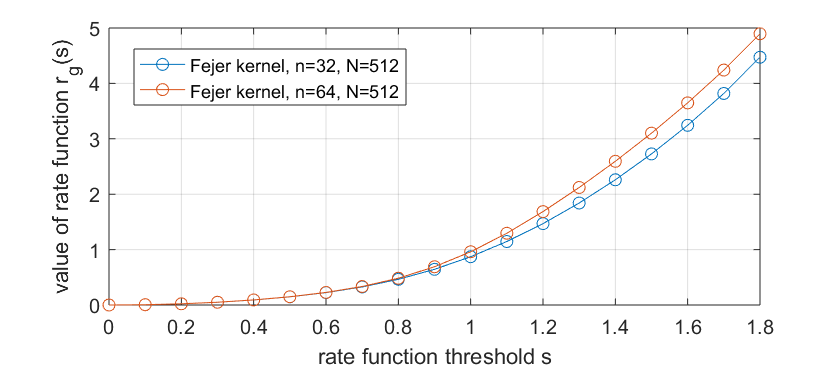
An overview of the paper is as follows. Section 2 briefly reviews results from [8] concerning the spectral stability of twisted quasi-compact operators in the sense of [23]. In Section 3 we state the abstract requirements for the Nagaev-Guivarc’h method to guarantee a central limit theorem and large deviation principle, and state an abstract hypothesis that yields stability of the variance and rate function using a modification of the abstract stability result from [8]. In Section 4 we briefly introduce the functional analytic setting of Gouëzel and Liverani [14] and verify the abstract hypothesis for Anosov maps in this setting. We then obtain stability of the rate function for Anosov diffeomorphisms under deterministic perturbations; see Theorem 4.4. Section 5 introduces our first Fourier-analytic scheme, which has wide applicability due to additional mollification, allowing the scheme to “smooth away” the complications of hyperbolic dynamics. Proposition 5.3 verifies that there is a sequence of Fourier projections of mollified transfer operators that satisfy the abstract stability hypotheses and Theorem 5.5 states the corresponding stability results. In Section 6 we introduce our second scheme, which removes the mollification step for Anosov maps with approximately constant stable and unstable directions; we obtain a pure (weighted) Fourier projection method based on the Fejér kernel. We may subject the transfer operator to stochastic kernels with relaxed regularity requirements (compared to Section 5) and full (but sufficiently decaying) support and still obtain the abstract stability hypotheses; see Proposition 6.1. Theorem 6.3 summarises the stability results that are obtained, and Corollary 6.4 addresses the perturbation arising from approximation with Fejér kernels. We conclude in Section 7 by implementing the above schemes on a nonlinear perturbation of Arnold’s cat map. We compare our Fourier-based estimates of the SRB measure and the variance with estimates from a (non-rigorous) pure Ulam method, and compute Fourier-based estimates of the rate function. To the authors’ knowledge, this constitutes the first rigorous computation of the variance and rate function of an Anosov map.

2 A review of the spectral stability of twisted quasi-compact operators

In this section we review the theory of spectral stability of quasi-compact operators from [23] and the corresponding results for twisted operators from [8]. Let (E,‖⋅‖)(E,\left\lVert\cdot\right\rVert) be a (complex) Banach space, denote by L⁡(E)L(E) the bounded linear operators on EE, and let A∈L⁡(E)A\in L(E). Denote the spectrum of AA by σ⁡(A)\sigma(A). The essential spectrum of AA is

σe​s​s​(A)={ω∈σ⁡(A):ω is not an eigenvalue of A of finite algebraic multiplicity}.\sigma_{ess}(A)=\{\omega\in\sigma(A):\text{$\omega$ is not an eigenvalue of $A$ of finite algebraic multiplicity}\}.

Denote the spectral radius and essential spectral radius of AA by ρ⁡(A)\rho(A) and ρe​s​s​(A)\rho_{ess}(A), respectively. We say that AA is quasi-compact if ρe​s​s​(A)<ρ​(A)\rho_{ess}(A)<\rho(A). If AA is quasi-compact and σ⁡(A)∩{ω:|ω|=ρ⁡(A)}\sigma(A)\cap\{\omega:\left\lvert\omega\right\rvert=\rho(A)\} consists of a single simple eigenvalue λ\lambda then we call AA simple and λ\lambda the leading eigenvalue of AA. In this case AA has decomposition [19, III.6.4-5]

A=λ​Π+N,A=\lambda\Pi+N, (1)

where Π\Pi is the rank-one eigenprojection corresponding to λ\lambda, N∈L⁡(E)N\in L(E) is such that ρ⁡(N)<ρ⁡(A)\rho(N)<\rho(A), and N​Π=Π​N=0N\Pi=\Pi N=0. We call (1) the quasi-compact decomposition of AA.

Let |⋅|\left\lvert\cdot\right\rvert be a norm on EE such that the closed, unit ball in (E,‖⋅‖)(E,\left\lVert\cdot\right\rVert) is relatively compact in the topology of |⋅|\left\lvert\cdot\right\rvert. After possibly scaling |⋅|\left\lvert\cdot\right\rvert, we may assume that |⋅|≤‖⋅‖\left\lvert\cdot\right\rvert\leq\left\lVert\cdot\right\rVert. Define the norm |||⋅|||{\left|\kern-1.07639pt\left|\kern-1.07639pt\left|\cdot\right|\kern-1.07639pt\right|\kern-1.07639pt\right|} on L⁡(E)L(E) by

‖|A|‖=sup‖f‖=1|A​f|.{\left|\kern-1.07639pt\left|\kern-1.07639pt\left|A\right|\kern-1.07639pt\right|\kern-1.07639pt\right|}=\sup_{\left\lVert f\right\rVert=1}\left\lvert Af\right\rvert.

It is classical that if AA is a simple quasi-compact operator and A′A^{\prime} is sufficiently close to AA in L⁡(E)L(E) then A′A^{\prime} is also a simple quasi-compact operator with leading eigenvalue close to λ\lambda (see e.g. [19, IV.3.5]). However, the condition of closeness in L⁡(E)L(E) is seldom satisfied by applications in dynamical systems. In [23], Keller and Liverani showed that if A′A^{\prime} is close to AA in the weaker topology of |||⋅|||{\left|\kern-1.07639pt\left|\kern-1.07639pt\left|\cdot\right|\kern-1.07639pt\right|\kern-1.07639pt\right|}, both operators obey a Lasota-Yorke inequality, and growth restrictions are placed on the (various) operator norms of iterates of AA and A′A^{\prime}, then one can recover appropriately modified versions of the spectral stability results from operator norm based perturbation theory. We now detail the requirements for these results, referring to [23] for exact statements.

Definition 2.1.

A family of operators {Aϵ}ϵ≥0⊆L⁡(E)\{A_{\epsilon}\}_{\epsilon\geq 0}\subseteq L(E) satisfies the Keller-Liverani (KL) condition if each of the following is satisfied:

  1. (KL1)

    There exists a monotone upper-semicontinuous function τ:[0,∞)→[0,∞)\tau:[0,\infty)\to[0,\infty) such that τ⁡(ϵ)>0\tau(\epsilon)>0 whenever ϵ>0\epsilon>0, ‖|Aϵ−A0|‖≤τ⁡(ϵ){\left|\kern-1.07639pt\left|\kern-1.07639pt\left|A_{\epsilon}-A_{0}\right|\kern-1.07639pt\right|\kern-1.07639pt\right|}\leq\tau(\epsilon), and limϵ→0τ⁡(ϵ)=0\lim_{\epsilon\to 0}\tau(\epsilon)=0.

  2. (KL2)

    There exists C1,K1>0C_{1},K_{1}>0 such that |Aϵn|≤C1​K1n\left\lvert A_{\epsilon}^{n}\right\rvert\leq C_{1}K_{1}^{n} for every ϵ≥0\epsilon\geq 0 and n∈ℕn\in\mathbb{N}.

  3. (KL3)

    There exists C2,C3,K2>0C_{2},C_{3},K_{2}>0 and α∈(0,1)\alpha\in(0,1) such that

    ‖Aϵn​f‖≤C2​αn​‖f‖+C3​K2n​|f|\left\lVert A_{\epsilon}^{n}f\right\rVert\leq C_{2}\alpha^{n}\left\lVert f\right\rVert+C_{3}K_{2}^{n}\left\lvert f\right\rvert (2)

    for every ϵ≥0\epsilon\geq 0, f∈Ef\in E and n∈ℕn\in\mathbb{N}.

Remark 2.2.

If rates of convergence are not required, then it suffices to prove that ‖|Aϵ−A0|‖→0{\left|\kern-1.07639pt\left|\kern-1.07639pt\left|A_{\epsilon}-A_{0}\right|\kern-1.07639pt\right|\kern-1.07639pt\right|}\to 0 instead of constructing the function τ\tau in (KL1). After possibly passing to a sub-family {Aϵ}ϵ∈[0,ϵ′)\{A_{\epsilon}\}_{\epsilon\in[0,\epsilon^{\prime})} for some ϵ′>0\epsilon^{\prime}>0, the two conditions are equivalent. We will use this fact frequently without further comment.

Instead of considering a single simple quasi-compact operator, one sometimes considers an analytic operator-valued map A⁡(⋅):D→L⁡(E)A(\cdot):D\to L(E), where D⊆ℂD\subseteq\mathbb{C} is an open neighbourhood of 0 and A⁡(0)A(0) is quasi-compact and simple. In this case, classical analytic perturbation theory for linear operators [19] posits the existence of some δ>0\delta>0 such that A⁡(z)A(z) is a simple quasi-compact operator for each z∈Dδ={ω:|ω|<δ}z\in D_{\delta}=\{\omega:\left\lvert\omega\right\rvert<\delta\}. Moreover, the quasi-compact decomposition of A⁡(z)A(z) depends analytically on zz i.e. there are analytic maps λ⁡(⋅):Dδ→ℂ\lambda(\cdot):D_{\delta}\to\mathbb{C}, Π⁡(⋅):Dδ→L⁡(E)\Pi(\cdot):D_{\delta}\to L(E), and N⁡(⋅):Dδ→L⁡(E)N(\cdot):D_{\delta}\to L(E) such that A⁡(z)A(z) has quasi-compact decomposition A⁡(z)=λ⁡(z)​Π​(z)+N⁡(z)A(z)=\lambda(z)\Pi(z)+N(z). In [8] the authors considered the question of spectral stability of such analytic operator-valued maps under conditions similar to (KL) and when the analytic families are induced by a ‘twist’.

Definition 2.3.

If M:D→L⁡(E)M:D\to L(E) is analytic on an open neighbourhood D⊆ℂD\subseteq\mathbb{C} of 0 and M⁡(0)M(0) is the identity, then we call MM a twist. If A∈L⁡(E)A\in L(E) then the operators A⁡(z):=A​M​(z)A(z):=AM(z) are said to be twisted by MM. We say that MM is compactly |⋅|\left\lvert\cdot\right\rvert-bounded if for every compact V⊆DV\subseteq D we have

supz∈V|M⁡(z)|<∞.\sup_{z\in V}\left\lvert M(z)\right\rvert<\infty.

We state a version of [8, Theorem 2.6] concerning the spectral stability of twisted quasi-compact operators.

Theorem 2.4 ([8, Theorem 2.6]).

Let {Aϵ}ϵ≥0\{A_{\epsilon}\}_{\epsilon\geq 0} satisfy (KL), where A0A_{0} is a simple quasi-compact operator with leading eigenvalue λ0\lambda_{0} satisfying α<|λ0|\alpha<\left\lvert\lambda_{0}\right\rvert, and let M:D→ℂM:D\to\mathbb{C} be a compactly |⋅|\left\lvert\cdot\right\rvert-bounded twist. Then there exists θ,ϵ′>0\theta,\epsilon^{\prime}>0 and, for each ϵ∈[0,ϵ′]\epsilon\in[0,\epsilon^{\prime}], analytic functions λϵ​(⋅):Dθ→ℂ\lambda_{\epsilon}(\cdot):D_{\theta}\to\mathbb{C}, Πϵ​(⋅):Dθ→L⁡(E)\Pi_{\epsilon}(\cdot):D_{\theta}\to L(E), and Nϵ​(⋅):Dθ→L⁡(E)N_{\epsilon}(\cdot):D_{\theta}\to L(E) such that Aϵ​(z)A_{\epsilon}(z) is a simple quasi-compact operator with decomposition Aϵ​(z)=λϵ​(z)​Πϵ​(z)+Nϵ​(z)A_{\epsilon}(z)=\lambda_{\epsilon}(z)\Pi_{\epsilon}(z)+N_{\epsilon}(z) whenever z∈Dθz\in D_{\theta}. Additionally, for each n∈ℕn\in\mathbb{N} we have the following convergence as ϵ→0\epsilon\to 0 on DθD_{\theta}:

  1. 1.

    λϵ(n)​(⋅)\lambda_{\epsilon}^{(n)}(\cdot) converges uniformly to λ0(n)​(⋅)\lambda_{0}^{(n)}(\cdot).

  2. 2.

    Πϵ(n)​(⋅)\Pi_{\epsilon}^{(n)}(\cdot) converges uniformly to Π0(n)​(⋅)\Pi_{0}^{(n)}(\cdot) in |||⋅|||{\left|\kern-1.07639pt\left|\kern-1.07639pt\left|\cdot\right|\kern-1.07639pt\right|\kern-1.07639pt\right|}.

  3. 3.

    Nϵ(n)​(⋅)N_{\epsilon}^{(n)}(\cdot) converges uniformly to N0(n)​(⋅)N_{0}^{(n)}(\cdot) in |||⋅|||{\left|\kern-1.07639pt\left|\kern-1.07639pt\left|\cdot\right|\kern-1.07639pt\right|\kern-1.07639pt\right|}.

We finish this section with a result concerning the robustness of the condition (KL) to perturbations that are simultaneously small in the operator norms ‖⋅‖\left\lVert\cdot\right\rVert and |⋅|\left\lvert\cdot\right\rvert, which we will frequently use in the sequel.

Proposition 2.5.

Suppose that {Aϵ}ϵ≥0\{A_{\epsilon}\}_{\epsilon\geq 0} satisfies (KL) and {Bϵ}ϵ∈[0,ϵ1)⊆L⁡(E)\{B_{\epsilon}\}_{\epsilon\in[0,\epsilon_{1})}\subseteq L(E) satisfies B0=0B_{0}=0, limϵ→0‖Bϵ‖=0\lim_{\epsilon\to 0}\left\lVert B_{\epsilon}\right\rVert=0 and supϵ∈[0,ϵ1)|Bϵ|<∞\sup_{\epsilon\in[0,\epsilon_{1})}\left\lvert B_{\epsilon}\right\rvert<\infty. Then there exists ϵ2∈(0,ϵ1)\epsilon_{2}\in(0,\epsilon_{1}) so that {Aϵ+Bϵ}ϵ∈[0,ϵ2)\{A_{\epsilon}+B_{\epsilon}\}_{\epsilon\in[0,\epsilon_{2})} satisfies (KL).

Proof.

We prove (KL1), (KL2) and (KL3) separately.

(KL1)

As ‖Bϵ‖→0\left\lVert B_{\epsilon}\right\rVert\to 0, there exists ϵ′>0\epsilon^{\prime}>0 so that supϵ∈[0,ϵ′)‖Bϵ‖<∞\sup_{\epsilon\in[0,\epsilon^{\prime})}\left\lVert B_{\epsilon}\right\rVert<\infty. As {Aϵ}ϵ≥0\{A_{\epsilon}\}_{\epsilon\geq 0} satisfies (KL1), {Bϵ}ϵ∈[0,ϵ′)\{B_{\epsilon}\}_{\epsilon\in[0,\epsilon^{\prime})} is bounded in L⁡(E)L(E), ‖Bϵ‖→0\left\lVert B_{\epsilon}\right\rVert\to 0, and

‖|Aϵ+Bϵ−A0|‖≤‖|Aϵ−A0|‖+‖Bϵ‖,{\left|\kern-1.07639pt\left|\kern-1.07639pt\left|A_{\epsilon}+B_{\epsilon}-A_{0}\right|\kern-1.07639pt\right|\kern-1.07639pt\right|}\leq{\left|\kern-1.07639pt\left|\kern-1.07639pt\left|A_{\epsilon}-A_{0}\right|\kern-1.07639pt\right|\kern-1.07639pt\right|}+\left\lVert B_{\epsilon}\right\rVert,

it is clear that (KL1) is satisfied.

(KL2)

As {Aϵ}ϵ≥0\{A_{\epsilon}\}_{\epsilon\geq 0} satisfies (KL2) and supϵ∈[0,ϵ1)|Bϵ|<∞\sup_{\epsilon\in[0,\epsilon_{1})}\left\lvert B_{\epsilon}\right\rvert<\infty, we have

supϵ∈[0,ϵ1)|Aϵ+Bϵ|≤C1​K+supϵ∈[0,ϵ1)|Bϵ|<∞.\sup_{\epsilon\in[0,\epsilon_{1})}\left\lvert A_{\epsilon}+B_{\epsilon}\right\rvert\leq C_{1}K+\sup_{\epsilon\in[0,\epsilon_{1})}\left\lvert B_{\epsilon}\right\rvert<\infty.

The required bound follows by iterating this inequality.

(KL3)

By expanding (Aϵ+Bϵ)n(A_{\epsilon}+B_{\epsilon})^{n}, applying a counting argument, and using (KL3) for {Aϵ}ϵ≥0\{A_{\epsilon}\}_{\epsilon\geq 0} we have

‖(Aϵ+Bϵ)n​f‖≤‖Aϵn​f‖+∑k=0n−1n!k!​(n−k)!​‖Aϵ‖k​‖Bϵ‖n−k​‖f‖≤C2​αn​‖f‖+C3​K2n​|f|+2n​∑k=0n−1‖Aϵ‖k​‖Bϵ‖n−k​‖f‖.\begin{split}\left\lVert(A_{\epsilon}+B_{\epsilon})^{n}f\right\rVert&\leq\left\lVert A_{\epsilon}^{n}f\right\rVert+\sum_{k=0}^{n-1}\frac{n!}{k!(n-k)!}\left\lVert A_{\epsilon}\right\rVert^{k}\left\lVert B_{\epsilon}\right\rVert^{n-k}\left\lVert f\right\rVert\\ &\leq C_{2}\alpha^{n}\left\lVert f\right\rVert+C_{3}K_{2}^{n}\left\lvert f\right\rvert+2^{n}\sum_{k=0}^{n-1}\left\lVert A_{\epsilon}\right\rVert^{k}\left\lVert B_{\epsilon}\right\rVert^{n-k}\left\lVert f\right\rVert.\end{split} (3)

Let β∈(α,1)\beta\in(\alpha,1) and choose n∈ℕn\in\mathbb{N} so that C1​αn<βnC_{1}\alpha^{n}<\beta^{n}. As (KL3) holds for {Aϵ}ϵ≥0\{A_{\epsilon}\}_{\epsilon\geq 0}, it follows that {Aϵ}ϵ≥0\{A_{\epsilon}\}_{\epsilon\geq 0} is bounded in L⁡(E)L(E). Hence, as ‖Bϵ‖→0\left\lVert B_{\epsilon}\right\rVert\to 0, there exists ϵ′′>0\epsilon^{\prime\prime}>0 so that for every ϵ∈[0,ϵ′′)\epsilon\in[0,\epsilon^{\prime\prime}) we have

C1​αn+2n​∑k=0n−1‖Aϵ‖k​‖Bϵ‖n−k≤βn.C_{1}\alpha^{n}+2^{n}\sum_{k=0}^{n-1}\left\lVert A_{\epsilon}\right\rVert^{k}\left\lVert B_{\epsilon}\right\rVert^{n-k}\leq\beta^{n}.

By applying (2) to (3) for all ϵ∈[0,ϵ′′)\epsilon\in[0,\epsilon^{\prime\prime}) we have

‖(Aϵ+Bϵ)n​f‖≤βn​‖f‖+C3​K2n​|f|.\left\lVert(A_{\epsilon}+B_{\epsilon})^{n}f\right\rVert\leq\beta^{n}\left\lVert f\right\rVert+C_{3}K_{2}^{n}\left\lvert f\right\rvert. (4)

Using (KL2) for {Aϵ+Bϵ}ϵ∈[0,ϵ1)\{A_{\epsilon}+B_{\epsilon}\}_{\epsilon\in[0,\epsilon_{1})} one may iterate (4) to obtain for all ϵ∈[0,ϵ′′)\epsilon\in[0,\epsilon^{\prime\prime}) and k∈ℤ+k\in\mathbb{Z}^{+} that

‖(Aϵ+Bϵ)n​k​f‖≤βn​k​‖f‖+C4​K3n​k​|f|,\left\lVert(A_{\epsilon}+B_{\epsilon})^{nk}f\right\rVert\leq\beta^{nk}\left\lVert f\right\rVert+C_{4}K_{3}^{nk}\left\lvert f\right\rvert, (5)

where C4,K3>0C_{4},K_{3}>0 are independent of kk and ϵ\epsilon. In the present setting, supϵ∈[0,ϵ′′)‖Aϵ+Bϵ‖\sup_{\epsilon\in[0,\epsilon^{\prime\prime})}\left\lVert A_{\epsilon}+B_{\epsilon}\right\rVert is finite. Using this fact one easily obtains (KL3) from (5). ∎

3 Stability of the statistical properties of dynamical systems via the naive Nagaev-Guivarc’h method

In [8] it is shown that when a dynamical system satisfies a central limit theorem or large deviation principle via the Nagaev-Guivarc’h method, then the variance and rate function associated with these statistical laws are stable under perturbations satisfying (KL). However, the the method as formulated in [8] (see also [15, 1]) is occasionally inapplicable due to some technical requirements; for example, it is required that the Perron-Frobenius operator is quasi-compact on a Banach algebra, and that the Banach space in question is a subspace of L1L^{1}. Neither condition is generally verified by the transfer operator associated to Anosov maps on any known Banach space. In [13] Gouëzel details the naive Nagaev-Guivarc’h method, which circumvents some of these shortcomings with a more abstract formulation of the method. In this section we recall how a CLT and LDP may be obtained via the naive Nagaev-Guivarc’h method. In Theorem 3.5 we show that when the method is compatible with the stability theory for twisted quasi-compact operators detailed in Section 2, then the variance of the CLT and the rate function of the LDP are stable to perturbations of the type (KL). In what follows {Yk}k∈ℕ\{Y_{k}\}_{k\in\mathbb{N}} is a sequence of real random variables with partial sums Sn=∑k=0n−1YkS_{n}=\sum_{k=0}^{n-1}Y_{k} satisfying limn→∞𝔼⁡(Sn)/n=0\lim_{n\to\infty}\mathbb{E}(S_{n})/n=0.

Theorem 3.1 (Central limit theorem [13, Theorem 2.4]).

If there exist a Banach space EE, operator-valued map A⁡(⋅):I→L⁡(E)A(\cdot):I\to L(E), where II is a real open neighbourhood of 0, and ζ∈E\zeta\in E, ν∈E∗\nu\in E^{*} such that:

  1. 1.

    A⁡(0)A(0) is a simple quasi-compact operator with ρ⁡(A⁡(0))=1\rho(A(0))=1.

  2. 2.

    The mapping t↦A⁡(t)t\mapsto A(t) is 𝒞2\mathcal{C}^{2}.

  3. 3.

    𝔼⁡(ei​t​Sn)=ν​A​(t)n​ζ\mathbb{E}(e^{itS_{n}})=\nu A(t)^{n}\zeta for all n∈ℕn\in\mathbb{N} and t∈It\in I.

Then {Yk}k∈ℕ\{Y_{k}\}_{k\in\mathbb{N}} satisfies a CLT: there exists σ2≥0\sigma^{2}\geq 0 such that Sn/nS_{n}/\sqrt{n} converges in distribution to a N⁡(0,σ2)N(0,\sigma^{2}) random variable as n→∞n\to\infty.

Theorem 3.2 (Large deviation principle [10, Remark 2.3]).

If there exist a Banach space EE, operator-valued map A⁡(⋅):I→L⁡(E)A(\cdot):I\to L(E), where II is a real open neighbourhood of 0, and ζ∈E\zeta\in E, ν∈E∗\nu\in E^{*} such that:

  1. 1.

    A⁡(0)A(0) is a simple quasi-compact operator with ρ⁡(A⁡(0))=1\rho(A(0))=1.

  2. 2.

    The mapping t↦A⁡(t)t\mapsto A(t) is 𝒞1\mathcal{C}^{1} and t↦ln⁡ρ⁡(A⁡(t))t\mapsto\ln\rho(A(t)) is strictly convex in some neighbourhood of 0.

  3. 3.

    𝔼⁡(et​Sn)=ν​A​(t)n​ζ\mathbb{E}(e^{tS_{n}})=\nu A(t)^{n}\zeta for all n∈ℕn\in\mathbb{N} and t∈It\in I.

Then {Yk}k∈ℕ\{Y_{k}\}_{k\in\mathbb{N}} satisfies a LDP: there exists a non-negative, continuous and convex rate function r:J→ℝr:J\to\mathbb{R}, where JJ is an open neighbourhood of 00, such that for every ϵ∈J∩(0,∞)\epsilon\in J\cap(0,\infty) we have

limn→∞1n​ln⁡Prob⁡(Sn≥n​ϵ)=−r⁡(ϵ).\lim_{n\to\infty}\frac{1}{n}\ln\Prob(S_{n}\geq n\epsilon)=-r(\epsilon).
Remark 3.3.

As stated, Theorem 3.2 differs slightly to the result in [10, Remark 2.3], however a straightforward modification of the arguments from [10] readily yields Theorem 3.2.

Both the CLT and LDP are parameterised, and under the settings of Theorems 3.1 and 3.2 these parameters are determined by the spectral data of A⁡(t)A(t) as follows. As t↦A⁡(t)t\mapsto A(t) is 𝒞k\mathcal{C}^{k} (k=1,2k=1,2) and A⁡(0)A(0) is a simple quasi-compact operator, by [13, Proposition 2.3] there exists θ>0\theta>0 and 𝒞k\mathcal{C}^{k} maps λ⁡(⋅):(−θ,θ)→ℂ\lambda(\cdot):(-\theta,\theta)\to\mathbb{C}, Π⁡(⋅):(−θ,θ)→L⁡(E)\Pi(\cdot):(-\theta,\theta)\to L(E), and N⁡(⋅):(−θ,θ)→L⁡(E)N(\cdot):(-\theta,\theta)\to L(E) such that for for t∈(−θ,θ)t\in(-\theta,\theta) the operator A⁡(t)A(t) is quasi-compact and simple with leading eigenvalue λ⁡(t)\lambda(t) and decomposition A⁡(t)=λ⁡(t)​Π​(t)+N⁡(t)A(t)=\lambda(t)\Pi(t)+N(t). The variance of CLT is

σ2=λ(2)​(0),\sigma^{2}=\lambda^{(2)}(0), (6)

and the rate function of the LDP is

r⁡(s)=supt∈(−θ,θ)(s​t−ln⁡|λ⁡(t)|).r(s)=\sup_{t\in(-\theta,\theta)}(st-\ln\left\lvert\lambda(t)\right\rvert).

Moreover, due to the strict convexity and continuous differentiability of t↦ln⁡|λ⁡(t)|t\mapsto\ln\left\lvert\lambda(t)\right\rvert on (−θ,θ)(-\theta,\theta), and the application of the local Gartner-Ellis Theorem [15, Lemma XIII.2] used to obtain Theorem 3.2, we have that the domain of the rate function is

(dd​z​ln⁡|λ⁡(z)||z=−θ,dd​z​ln⁡|λ⁡(z)||z=θ).\left({\left.\kern-1.2pt\frac{\mathrm{d}}{\mathrm{d}z}\ln\left\lvert\lambda(z)\right\rvert\vphantom{\big|}\right|_{z=-\theta}},{\left.\kern-1.2pt\frac{\mathrm{d}}{\mathrm{d}z}\ln\left\lvert\lambda(z)\right\rvert\vphantom{\big|}\right|_{z=\theta}}\right). (7)

In Theorem 3.1 the characteristic function of SnS_{n} is encoded by ν​A​(t)n​ζ\nu A(t)^{n}\zeta whilst in Theorem 3.2 it is the moment-generating function of SnS_{n} that is encoded. These settings are frequently unified by the following hypothesis:

Hypothesis 3.4.

Suppose that {Yk}k∈ℕ\{Y_{k}\}_{k\in\mathbb{N}} is a sequence of real random variables with partial sums Sn=∑k=0n−1YkS_{n}=\sum_{k=0}^{n-1}Y_{k} satisfying limn→∞𝔼⁡(Sn)/n=0\lim_{n\to\infty}\mathbb{E}(S_{n})/n=0. We say that {Yk}k∈ℕ\{Y_{k}\}_{k\in\mathbb{N}} satisfies Hypothesis 3.4 if there exists a Banach space (E,‖⋅‖)(E,\left\lVert\cdot\right\rVert), ζ∈E\zeta\in E, ν∈E∗\nu\in E^{*}, and an analytic operator-valued map A:D↦L⁡(E)A:D\mapsto L(E), where D⊆ℂD\subseteq\mathbb{C} is an open neighbourhood of 00, such that A⁡(0)A(0) is a simple quasi-compact operator, ρ⁡(A⁡(0))=1\rho(A(0))=1, t↦ρ⁡(A⁡(t))t\mapsto\rho(A(t)) is strictly convex in some real neighbourhood of 0, and

𝔼⁡(ez​Sn)=ν​A​(z)n​ζ\mathbb{E}(e^{zS_{n}})=\nu A(z)^{n}\zeta

for every z∈Dz\in D and n∈ℕn\in\mathbb{N}.

It is clear that if Hypothesis 3.4 holds then Theorems 3.1 and 3.2 both hold i.e. {Yk}k∈ℕ\{Y_{k}\}_{k\in\mathbb{N}} satisfies a CLT and LDP. Hypothesis 3.4 is frequently verified by applications of the naive Nagaev-Guivarc’h method to dynamical systems. In addition, in these applications the map z↦A⁡(z)z\mapsto A(z) arises from a twist i.e. there exists a twist M:D↦L⁡(E)M:D\mapsto L(E) such that A⁡(z)=A⁡(0)​M​(z)A(z)=A(0)M(z). In this case we can apply Theorem 2.4 to obtain stability of the variance and rate function with respect to perturbations satisfying (KL).

Theorem 3.5.

Let {Yk}k∈ℕ\{Y_{k}\}_{k\in\mathbb{N}} be a sequence of real random variables satisfying Hypothesis 3.4. Suppose that |⋅|\left\lvert\cdot\right\rvert is a second norm on EE so that the closed, unit ball in (E,‖⋅‖)(E,\left\lVert\cdot\right\rVert) is relatively compact with respect to |⋅|\left\lvert\cdot\right\rvert and that there exists a compactly |⋅|\left\lvert\cdot\right\rvert-bounded twist M:D→L⁡(E)M:D\to L(E) such that A⁡(z)=A⁡(0)​M​(z)A(z)=A(0)M(z). If {Aϵ}ϵ≥0\{A_{\epsilon}\}_{\epsilon\geq 0} satisfies (KL), where A0=A⁡(0)A_{0}=A(0), then there exists θ,ϵ′>0\theta,\epsilon^{\prime}>0 and, for every ϵ∈[0,ϵ′]\epsilon\in[0,\epsilon^{\prime}], analytic maps λϵ​(⋅):Dθ→ℂ\lambda_{\epsilon}(\cdot):D_{\theta}\to\mathbb{C}, Πϵ​(⋅):Dθ→L⁡(E)\Pi_{\epsilon}(\cdot):D_{\theta}\to L(E) and Nϵ​(⋅):Dθ→L⁡(E)N_{\epsilon}(\cdot):D_{\theta}\to L(E) such that for every ϵ∈[0,ϵ′]\epsilon\in[0,\epsilon^{\prime}] and z∈Dθz\in D_{\theta} the operator Aϵ​(z)A_{\epsilon}(z) has quasi-compact decomposition Aϵ​(z)=λϵ​(z)​Πϵ​(z)+Nϵ​(z)A_{\epsilon}(z)=\lambda_{\epsilon}(z)\Pi_{\epsilon}(z)+N_{\epsilon}(z) and as ϵ→0\epsilon\to 0 the maps λϵ​(⋅)\lambda_{\epsilon}(\cdot), Πϵ​(⋅)\Pi_{\epsilon}(\cdot) and Nϵ​(⋅)N_{\epsilon}(\cdot) converge as in Theorem 2.4. Moreover, we have stability of the parameters of the CLT and LDP for {Yk}k∈ℕ\{Y_{k}\}_{k\in\mathbb{N}} in the following sense:

  1. 1.

    The variance is stable: limϵ→0λϵ(2)​(0)=σ2\lim_{\epsilon\to 0}\lambda_{\epsilon}^{(2)}(0)=\sigma^{2}.

  2. 2.

    The rate function is stable: for each sufficiently small compact subset UU of the domain of the rate function rgr_{g} there exists an interval V⊆(−θ,θ)V\subseteq(-\theta,\theta) so that

    limϵ→0supz∈V(s​z−log⁡|λϵ​(z)|)=r⁡(s)\lim_{\epsilon\to 0}\sup_{z\in V}(sz-\log\left\lvert\lambda_{\epsilon}(z)\right\rvert)=r(s)

    uniformly on UU.

Proof.

By Theorem 2.4 there exists θ,ϵ′>0\theta,\epsilon^{\prime}>0 and, for each ϵ∈[0,ϵ′]\epsilon\in[0,\epsilon^{\prime}], maps λϵ​(⋅),Πϵ​(⋅)\lambda_{\epsilon}(\cdot),\Pi_{\epsilon}(\cdot) and Nϵ​(⋅)N_{\epsilon}(\cdot) as required for Theorem 3.5. The proof of the stability of the variance follows from (6) and Theorem 2.4. After possibly reducing the value of θ\theta, so that the domain of the rate function is the one given in Theorem 3.2, the stability of the rate function follows from [8, Theorem 3.8 and Proposition 3.9] with some minor modifications that we will now discuss. In [8] it is required that Aϵ​(z)A_{\epsilon}(z) is positive for each ϵ≥0\epsilon\geq 0 and z∈ℝz\in\mathbb{R} so that λϵ​(z)\lambda_{\epsilon}(z) is positive too; we remove this assumption and consequently deal with |λϵ​(z)|\left\lvert\lambda_{\epsilon}(z)\right\rvert instead. By Theorem 2.4 and the reverse triangle inequality we have uniform convergence of |λϵ​(⋅)|\left\lvert\lambda_{\epsilon}(\cdot)\right\rvert to |λ0​(⋅)|\left\lvert\lambda_{0}(\cdot)\right\rvert on each compact subset of DθD_{\theta}. Although [8, Theorem 3.8] proves a Hölder estimate for the convergence of the rate functions, straightforward modifications to the proof yields uniform convergence as is required for Theorem 3.5. The proof of [8, Proposition 3.10] holds upon replacing [8, Lemma 3.9] with the condition that z↦ln⁡ρ⁡(ℒ⁡(z))z\mapsto\ln\rho(\mathcal{L}(z)) is strictly convex in a real neighbourhood of 00, and noting that z↦ln⁡|λ0​(z)|z\mapsto\ln\left\lvert\lambda_{0}(z)\right\rvert is 𝒞1\mathcal{C}^{1} on (−θ,θ)(-\theta,\theta). ∎

4 Stability of statistical limit laws for Anosov maps

It is classical that topologically transitive Anosov diffeomorphisms satisfy a central limit theorem and large deviation principle for sufficiently smooth observables: such results were first established by using Markov partitions to reduce to the case of subshifts of finite type [26, 27]. In order to apply the stability results from Section 3 to Anosov maps we require that these limit laws hold due to the naive Nagaev-Guivarc’h method; verifying this is the main point of this section. In particular, using the functional analytic setup in [14], we confirm that {g∘Tk}k∈ℕ\{g\circ T^{k}\}_{k\in\mathbb{N}} satisfies Hypothesis 3.4 for TT a 𝒞r+1\mathcal{C}^{r+1} Anosov map, r>1r>1, and appropriate observables gg. Theorem 3.5 then yields stability of the variance and rate function to perturbations of type (KL), which forms the basis for our results in Sections 5, 6 and 7.

4.1 The functional analytic setup of Gouëzel and Liverani

We review the functional analytic setup of [14]. Let d>1d>1 and XX be a dd-dimensional, 𝒞∞\mathcal{C}^{\infty}, compact, connected Riemannian manifold and T∈𝒞r+1​(X,X)T\in\mathcal{C}^{r+1}(X,X), r>1r>1, be an Anosov map. By using an adapted metric we may assume that νu>1\nu_{u}>1 is everywhere less than the local expansion of TT in the unstable direction, and νs<1\nu_{s}<1 is everywhere greater than the local contraction of TT in the stable direction (see [5, Proposition 5.2.2]). We review the construction of such a metric in Section 6.1. When TT has a unique SRB measure we denote it by μ\mu. Let Ω\Omega denote both the Riemannian measure on XX and the linear functional f↦∫f​𝑑Ωf\mapsto\int\!f\,\mathrm{d}\Omega. The transfer operator ℒ:𝒞r​(X,ℝ)→𝒞r​(X,ℝ)\mathcal{L}:\mathcal{C}^{r}(X,\mathbb{R})\to\mathcal{C}^{r}(X,\mathbb{R}) associated with TT is defined by

∫(ℒ​h)⋅u​𝑑Ω=∫h⋅(u∘T)​𝑑Ω,\int\!(\mathcal{L}h)\cdot u\,\mathrm{d}\Omega=\int\!h\cdot(u\circ T)\,\mathrm{d}\Omega, (8)

where u,h∈𝒞r​(X,ℝ)u,h\in\mathcal{C}^{r}(X,\mathbb{R}). For ℒ\mathcal{L} to have ‘good’ spectral properties it is necessary to consider it as an operator on an appropriately chosen anisotropic Banach space. We now describe the construction of such a space from [14]. Denote by Σ\Sigma the set of admissible leaves (see [14, Section 3] for the full definition). For each W∈ΣW\in\Sigma we denote the collection of 𝒞r\mathcal{C}^{r} vector fields that are defined on a neighbourhood of WW by 𝒱r​(W)\mathcal{V}^{r}(W), and by 𝒞0q​(W,ℝ)\mathcal{C}^{q}_{0}(W,\mathbb{R}) the set of functions in 𝒞q​(W,ℝ)\mathcal{C}^{q}(W,\mathbb{R}) that vanish on a neighbourhood of ∂W\partial W. For h∈𝒞r​(X,ℝ)h\in\mathcal{C}^{r}(X,\mathbb{R}), q>0q>0, p∈ℕp\in\mathbb{N} with p≤rp\leq r let

‖h‖p,q−=supW∈Σsupv1,…​vp∈𝒱r​(W)|vi|𝒞r≤1supφ∈𝒞0q​(W,ℝ)|φ|𝒞q≤1∫W(v1​…​vp​h)⋅φ.\left\lVert h\right\rVert^{-}_{p,q}=\sup_{W\in\Sigma}\,\sup_{\begin{subarray}{c}v_{1},\dots v_{p}\in\mathcal{V}^{r}(W)\\ \left\lvert v_{i}\right\rvert_{\mathcal{C}^{r}}\leq 1\end{subarray}}\,\sup_{\begin{subarray}{c}\varphi\in\mathcal{C}^{q}_{0}(W,\mathbb{R})\\ \left\lvert\varphi\right\rvert_{\mathcal{C}^{q}}\leq 1\end{subarray}}\,\int_{W}(v_{1}\dots v_{p}h)\cdot\varphi.

Then

‖h‖p,q=sup0≤k≤p‖h‖k,q+k−=supp′≤p,q′≥q+p′‖h‖p′,q′−\left\lVert h\right\rVert_{p,q}=\sup_{0\leq k\leq p}\left\lVert h\right\rVert^{-}_{k,q+k}=\sup_{p^{\prime}\leq p,q^{\prime}\geq q+p^{\prime}}\left\lVert h\right\rVert^{-}_{p^{\prime},q^{\prime}} (9)

is a norm on 𝒞r​(X,ℝ)\mathcal{C}^{r}(X,\mathbb{R}). Denote by Bp,qB^{p,q} the completion of 𝒞r​(X,ℝ)\mathcal{C}^{r}(X,\mathbb{R}) under this norm. As the naive Nagaev-Guivarc’h method requires a complex Banach space, we consider the complexification Bℂp,qB^{p,q}_{\mathbb{C}} of the spaces Bp,qB^{p,q}. When endowed with the norm11 1 We abuse notation and denote the norm on Bℂp,qB^{p,q}_{\mathbb{C}} by ‖⋅‖p,q\left\lVert\cdot\right\rVert_{p,q}.

‖hr+i​hi‖p,q=max⁡{‖hr‖p,q,‖hi‖p,q},\left\lVert h_{r}+ih_{i}\right\rVert_{p,q}=\max\{\left\lVert h_{r}\right\rVert_{p,q},\left\lVert h_{i}\right\rVert_{p,q}\}, (10)

Bℂp,qB^{p,q}_{\mathbb{C}} is a complex Banach space. It is on this space that the operator ℒ\mathcal{L} is quasi-compact.

Theorem 4.1 ([14, Theorem 2.3]).

If p∈ℤ+p\in\mathbb{Z}^{+} and q>0q>0 satisfy q+p<rq+p<r then the operator ℒ:Bℂp,q→Bℂp,q\mathcal{L}:B^{p,q}_{\mathbb{C}}\to B^{p,q}_{\mathbb{C}} has spectral radius one. In addition, ℒ\mathcal{L} is quasi-compact with ρe​s​s​(ℒ)⊆{ω∈ℂ:|ω|≤max⁡{νu−p,νsq}}\rho_{ess}(\mathcal{L})\subseteq\{\omega\in\mathbb{C}:\left\lvert\omega\right\rvert\leq\max\{\nu_{u}^{-p},\nu_{s}^{q}\}\}. Moreover, the eigenfunctions corresponding to eigenvalues of modulus 1 are distributions of order 0, i.e., measures. If the map is topologically transitive, then 1 is a simple eigenvalue and no other eigenvalues of modulus one are present.

4.2 The naive Nagaev-Guivarc’h method for Anosov maps

The main technical result of this section is Proposition 4.3, which verifies Hypothesis 3.4 in the setting of Section 4.1. As 1∈Bℂp,q1\in B^{p,q}_{\mathbb{C}}, for any g∈𝒞r​(X,ℝ)g\in\mathcal{C}^{r}(X,\mathbb{R}) we may define ez​ge^{zg} by the power series ∑k=0∞zk​gk/k!\sum_{k=0}^{\infty}z^{k}g^{k}/k!. We define Mg​(⋅):ℂ→L⁡(Bℂp,q)M_{g}(\cdot):\mathbb{C}\to L(B^{p,q}_{\mathbb{C}}) by setting Mg​(z)​(h)=ez​g​hM_{g}(z)(h)=e^{zg}h for h∈𝒞r​(X,ℂ)h\in\mathcal{C}^{r}(X,\mathbb{C}) and then passing to Bℂp,qB^{p,q}_{\mathbb{C}} by density.

Proposition 4.2.

Let p∈ℤ+p\in\mathbb{Z}^{+}, q>0q>0 satisfy p+q<rp+q<r. If g∈𝒞r​(X,ℝ)g\in\mathcal{C}^{r}(X,\mathbb{R}) and Mg:ℂ→L⁡(Bℂp,q)M_{g}:\mathbb{C}\to L(B^{p,q}_{\mathbb{C}}) is defined by Mg​(z)​(f)=ez​g​fM_{g}(z)(f)=e^{zg}f, then MgM_{g} is a compactly ‖⋅‖p−1,q+1\left\lVert\cdot\right\rVert_{p-1,q+1}-bounded twist.

By [14, Proposition 4.1] there is a continuous injection from Bℂp,qB^{p,q}_{\mathbb{C}} into 𝒟q′​(X)\mathcal{D}_{q}^{\prime}(X), the distributions of order at most qq. With this injection in mind, we can consider some elements of Bℂp,qB^{p,q}_{\mathbb{C}} as probability measures (exactly when they are probability measures in 𝒟q′​(X)\mathcal{D}_{q}^{\prime}(X)). Recall that g∈𝒞r​(X,ℝ)g\in\mathcal{C}^{r}(X,\mathbb{R}) is an L2​(μ)L^{2}(\mu)-coboundary if there is ϕ∈L2​(μ)\phi\in L^{2}(\mu) so that g=ϕ−ϕ∘Tg=\phi-\phi\circ T.

Proposition 4.3.

Assume that ℒ\mathcal{L} is a simple quasi-compact operator. Let p∈ℤ+p\in\mathbb{Z}^{+} and q>0q>0 satisfy q+p<rq+p<r. Let m∈Bp,qm\in B^{p,q} be a probability measure, and suppose g∈𝒞r​(X,ℝ)g\in\mathcal{C}^{r}(X,\mathbb{R}) satisfies ∫g​𝑑μ=0\int\!g\,\mathrm{d}\mu=0 and is not an L2​(μ)L^{2}(\mu)-coboundary. Define ℒ⁡(⋅):ℂ→L⁡(Bℂp,q)\mathcal{L}(\cdot):\mathbb{C}\to L(B^{p,q}_{\mathbb{C}}) by ℒ⁡(z)=ℒ​Mg​(z)\mathcal{L}(z)=\mathcal{L}M_{g}(z). Then {g∘Tk}k∈ℕ\{g\circ T^{k}\}_{k\in\mathbb{N}}, when considered on the probability space (X,m)(X,m), satisfies Hypothesis 3.4 with Banach space Bℂp,qB^{p,q}_{\mathbb{C}} and operator-valued map ℒ⁡(⋅)\mathcal{L}(\cdot).

With Proposition 4.3 in hand, by Theorems 3.1 and 3.2 we immediately obtain a CLT and LDP (on appropriate probability spaces) for {g∘Tk}k∈ℕ\{g\circ T^{k}\}_{k\in\mathbb{N}} whenever g∈𝒞r​(X,ℝ)g\in\mathcal{C}^{r}(X,\mathbb{R}) satisfies ∫g​𝑑μ=0\int\!g\,\mathrm{d}\mu=0 and is not an L2​(μ)L^{2}(\mu)-coboundary. Moreover, as MgM_{g} is a compactly ‖⋅‖p−1,q+1\left\lVert\cdot\right\rVert_{p-1,q+1}-bounded twist and the unit ball in Bℂp,qB^{p,q}_{\mathbb{C}} is relatively compact in ‖⋅‖p−1,q+1\left\lVert\cdot\right\rVert_{p-1,q+1} [14, Lemma 2.1], Theorem 3.5 yields stability of the variance and rate function with respect to perturbations of the type (KL). In Section 7 we use this fact to numerically approximate the statistical properties of Anosov maps on tori. For the moment we state following application, which extends [14, Theorem 2.8, Remark 2.11]. For y∈ℝy\in\mathbb{R} we denote by τy\tau_{y} the map x↦x+yx\mapsto x+y.

Theorem 4.4 (Stability of the rate function under deterministic perturbations).

Let T⁡(⋅)∈𝒞1​([0,1],𝒞r+1​(X,X))T(\cdot)\in\mathcal{C}^{1}([0,1],\mathcal{C}^{r+1}(X,X)) be such that T⁡(0)T(0) is a topologically transitive Anosov diffeomorphism. Let p∈ℤ+p\in\mathbb{Z}^{+} and q>0q>0 satisfy p+q<rp+q<r. Fix a probability measure m∈Bp,qm\in B^{p,q} and suppose g∈𝒞r​(X,ℝ)g\in\mathcal{C}^{r}(X,\mathbb{R}) satisfies ∫g​𝑑μ=0\int\!g\,\mathrm{d}\mu=0 and is not an L2​(μ)L^{2}(\mu)-coboundary. There exists ϵ>0\epsilon>0 and, for each t∈[0,ϵ]t\in[0,\epsilon], a number AtA_{t} and map rt:J−At→ℝr_{t}:J-A_{t}\to\mathbb{R}, where JJ is an open real neighbourhood of 0, so that {g∘T​(t)k−At}k∈ℕ\{g\circ T(t)^{k}-A_{t}\}_{k\in\mathbb{N}} satisfies a LDP on (X,m)(X,m) with rate function rtr_{t}, At→A0=0A_{t}\to A_{0}=0 and rt∘τ−At→r0r_{t}\circ\tau_{-A_{t}}\to r_{0} compactly on JJ.

We defer the proofs of Propositions 4.2 and 4.3, and Theorem 4.4 to Appendix A.

5 Approximating the statistical data of Anosov maps

In this section we introduce a scheme for approximating the spectrum of the Perron-Frobenius operator associated to an Anosov map on the dd-dimensional torus 𝕋d\mathbb{T}^{d}, which we identify with ℝd/ℤd\mathbb{R}^{d}/\mathbb{Z}^{d}. The scheme proceeds by convolving the Perron-Frobenius operator with a compactly supported mollifier, and then approximating the ‘smoothened’ operator using Fourier series. A similar idea is developed in [4], where Ulam’s method is considered instead of Fourier series and convergence of the SRB measure and variance are obtained under this scheme. We note that [4] did not include any computations (as we do, in Section 7) nor did they consider the stability of the rate function.

Throughout this section we adopt the setting, assumptions and notation of Section 4.1, and fix p∈ℤ+p\in\mathbb{Z}^{+} and q>0q>0 satisfying p+q<rp+q<r. Let Leb\Leb denote the normalised Haar measure on 𝕋d\mathbb{T}^{d}. For some ϵ1>0\epsilon_{1}>0, suppose that the family of stochastic kernels {qϵ}ϵ∈(0,ϵ1)⊆𝒞∞​(𝕋d,ℝ)\{q_{\epsilon}\}_{\epsilon\in(0,\epsilon_{1})}\subseteq\mathcal{C}^{\infty}(\mathbb{T}^{d},\mathbb{R}) satisfies the following conditions:

  1. (S1)

    qϵ≥0q_{\epsilon}\geq 0 and ∫qϵ​d​Leb=1\int\!q_{\epsilon}\,\mathrm{d}\Leb=1;

  2. (S2)

    The support of qϵq_{\epsilon} is contained in Bϵ​(0)B_{\epsilon}(0).

For such a family we define operators Qϵ:𝒞r​(𝕋d,ℂ)→𝒞r​(𝕋d,ℂ)Q_{\epsilon}:\mathcal{C}^{r}(\mathbb{T}^{d},\mathbb{C})\to\mathcal{C}^{r}(\mathbb{T}^{d},\mathbb{C}) by Qϵ​f=f∗qϵQ_{\epsilon}f=f*q_{\epsilon}. Recall that convolution is defined with respect to the Haar measure Leb\Leb on 𝕋d\mathbb{T}^{d}, which may differ from the measure Ω\Omega that is induced by the adapted metric. It is evident, however, that the Radon-Nikodym derivatives d​Lebd​Ω\frac{\mathrm{d}\Leb}{\mathrm{d}\Omega} and d​Ωd​Leb\frac{\mathrm{d}\Omega}{\mathrm{d}\Leb} both exist, and are elements of 𝒞∞​(𝕋d,ℝ)\mathcal{C}^{\infty}(\mathbb{T}^{d},\mathbb{R}). As a consequence we obtain the following characterisation of QϵQ_{\epsilon}:

Lemma 5.1.

QϵQ_{\epsilon} extends to a bounded operator Qϵ:Bℂp,q→𝒞∞​(𝕋d,ℂ)Q_{\epsilon}:B^{p,q}_{\mathbb{C}}\to\mathcal{C}^{\infty}(\mathbb{T}^{d},\mathbb{C}). Consequently, QϵQ_{\epsilon} is compact as an element of L⁡(Bℂp,q,𝒞m​(𝕋d,ℂ))L(B^{p,q}_{\mathbb{C}},\mathcal{C}^{m}(\mathbb{T}^{d},\mathbb{C})) for every m∈ℤ+m\in\mathbb{Z}^{+}. Moreover, QϵQ_{\epsilon} is compact as an element of L⁡(Bℂp,q)L(B^{p,q}_{\mathbb{C}}) and, for each m1,m2∈ℤ+m_{1},m_{2}\in\mathbb{Z}^{+}, as an element of L⁡(𝒞m1​(𝕋d,ℂ),𝒞m2​(𝕋d,ℂ))L(\mathcal{C}^{m_{1}}(\mathbb{T}^{d},\mathbb{C}),\mathcal{C}^{m_{2}}(\mathbb{T}^{d},\mathbb{C})).

Let ℒ0=ℒ\mathcal{L}_{0}=\mathcal{L} and, for each ϵ∈(0,ϵ1)\epsilon\in(0,\epsilon_{1}), let ℒϵ=Qϵ​ℒ0\mathcal{L}_{\epsilon}=Q_{\epsilon}\mathcal{L}_{0}, which is in L⁡(Bℂp,q)L(B^{p,q}_{\mathbb{C}}) by virtue of the previous lemma.

Lemma 5.2.

There exists ϵ2∈(0,ϵ1)\epsilon_{2}\in(0,\epsilon_{1}) so that {ℒϵ}ϵ∈[0,ϵ2)\{\mathcal{L}_{\epsilon}\}_{\epsilon\in[0,\epsilon_{2})} satisfies (KL) on Bℂp,qB^{p,q}_{\mathbb{C}} with |⋅|=‖⋅‖p−1,q+1\left\lvert\cdot\right\rvert=\left\lVert\cdot\right\rVert_{p-1,q+1}.

By Lemma 5.1, for each ϵ∈(0,ϵ1)\epsilon\in(0,\epsilon_{1}) the operator ℒϵ\mathcal{L}_{\epsilon} is compact and, for every m∈ℤ+m\in\mathbb{Z}^{+}, maps the unit ball of Bℂp,qB^{p,q}_{\mathbb{C}} into a bounded subset of 𝒞m​(𝕋d,ℂ)\mathcal{C}^{m}(\mathbb{T}^{d},\mathbb{C}). For this reason ℒϵ\mathcal{L}_{\epsilon} may be approximated with Fourier series for each ϵ>0\epsilon>0. For k=(k1,…,kd)∈ℤdk=(k_{1},\dots,k_{d})\in\mathbb{Z}^{d} we set ‖k‖∞=maxi⁡|ki|\left\lVert k\right\rVert_{\infty}=\max_{i}\left\lvert k_{i}\right\rvert and ‖k‖1=∑i|ki|\left\lVert k\right\rVert_{1}=\sum_{i}\left\lvert k_{i}\right\rvert. For each n∈ℤ+n\in\mathbb{Z}^{+} define Πn:𝒞⁡(𝕋d,ℂ)→𝒞⁡(𝕋d,ℂ)\Pi_{n}:\mathcal{C}(\mathbb{T}^{d},\mathbb{C})\to\mathcal{C}(\mathbb{T}^{d},\mathbb{C}) by

(Πn​f)​(x)=∑k∈ℤd‖k‖∞≤nf^​(k)​e2​π​i​x⋅k,(\Pi_{n}f)(x)=\sum_{\begin{subarray}{c}k\in\mathbb{Z}^{d}\\ \left\lVert k\right\rVert_{\infty}\leq n\end{subarray}}\hat{f}(k)e^{2\pi ix\cdot k},

where f^\hat{f} denotes the Fourier transform22 2 Specifically, f^(k)=∫𝕋df(x)e−2πix⋅kdLeb(x)\hat{f}(k)=\int_{\mathbb{T}^{d}}\!f(x)e^{-2\pi ix\cdot k}\,\mathrm{d}\Leb(x). of ff. For every ϵ∈(0,ϵ1)\epsilon\in(0,\epsilon_{1}) and n∈ℤ+n\in\mathbb{Z}^{+} let ℒϵ,n=Πn​ℒϵ\mathcal{L}_{\epsilon,n}=\Pi_{n}\mathcal{L}_{\epsilon}. To simplify our notation, we set ℒϵ,∞=ℒϵ\mathcal{L}_{\epsilon,\infty}=\mathcal{L}_{\epsilon}. Our main technical result for this section is the following.

Proposition 5.3.

There exists ϵ3∈(0,ϵ2)\epsilon_{3}\in(0,\epsilon_{2}) and a map N:[0,ϵ3)→ℕ∪{∞}N:[0,\epsilon_{3})\to\mathbb{N}\cup\{\infty\} with N−1​(∞)={0}N^{-1}(\infty)=\{0\}, so that for any map n:[0,ϵ3)→ℕ∪{∞}n:[0,\epsilon_{3})\to\mathbb{N}\cup\{\infty\} with n≥Nn\geq N the family of operators {ℒϵ,n⁡(ϵ)}ϵ∈[0,ϵ3)\{\mathcal{L}_{\epsilon,n(\epsilon)}\}_{\epsilon\in[0,\epsilon_{3})} satisfies (KL) on Bℂp,qB^{p,q}_{\mathbb{C}} with |⋅|=‖⋅‖p−1,q+1\left\lvert\cdot\right\rvert=\left\lVert\cdot\right\rVert_{p-1,q+1}.

Remark 5.4.

By Proposition 5.3 we may apply the results in [23] to {ℒϵ,n⁡(ϵ)}ϵ∈[0,ϵ3)\{\mathcal{L}_{\epsilon,n(\epsilon)}\}_{\epsilon\in[0,\epsilon_{3})}. Hence, all the isolated eigenvalues of ℒ\mathcal{L} with modulus strictly greater than the constant α\alpha in (2) are approximated by eigenvalues of ℒϵ,n⁡(ϵ)\mathcal{L}_{\epsilon,n(\epsilon)}, with error vanishing as ϵ→0\epsilon\to 0. When such an eigenvalue of ℒ\mathcal{L} is simple, we additionally have that the corresponding eigenprojection and eigenvector are approximated by those of ℒϵ,n⁡(ϵ)\mathcal{L}_{\epsilon,n(\epsilon)} in |||⋅|||{\left|\kern-1.07639pt\left|\kern-1.07639pt\left|\cdot\right|\kern-1.07639pt\right|\kern-1.07639pt\right|} and |⋅|\left\lvert\cdot\right\rvert, respectively.

Propositions 5.3 and 4.3 allow us to apply Theorem 3.5 to obtain the stability of the invariant measure, variance and rate function. We note that since Anosov diffeomorphisms on tori are mixing [20, Proposition 18.6.5], it follows that 11 is the only eigenvalue of ℒ\mathcal{L} of modulus 1, and is a simple eigenvalue. In particular TT has a unique SRB measure μ∈Bp,q\mu\in B^{p,q}, as required by Theorem 3.5.

Theorem 5.5.

Suppose that g∈𝒞r​(𝕋d,ℝ)g\in\mathcal{C}^{r}(\mathbb{T}^{d},\mathbb{R}) satisfies ∫g​𝑑μ=0\int\!g\,\mathrm{d}\mu=0 and is not a L2​(μ)L^{2}(\mu)-coboundary. Denote by Mg​(⋅):ℂ→L⁡(Bℂp,q)M_{g}(\cdot):\mathbb{C}\to L(B^{p,q}_{\mathbb{C}}) the map Mg​(z)​f=ez​g​fM_{g}(z)f=e^{zg}f. Let N,nN,n satisfy the conditions of Proposition 5.3. There exists θ,ϵ′>0\theta,\epsilon^{\prime}>0 so that for each ϵ∈[0,ϵ′)\epsilon\in[0,\epsilon^{\prime}) and z∈Dθz\in D_{\theta} the operator ℒϵ,n⁡(ϵ)​(z)\mathcal{L}_{\epsilon,n(\epsilon)}(z) is quasi-compact and simple with leading eigenvalue λϵ​(z)\lambda_{\epsilon}(z) depending analytically on zz. Moreover, we have stability of the following statistical data associated to TT and {g∘Tk}k∈ℕ\{g\circ T^{k}\}_{k\in\mathbb{N}}:

  1. 1.

    The invariant measure is stable: there exists eigenvectors vϵ∈Bℂp,qv_{\epsilon}\in B^{p,q}_{\mathbb{C}} of ℒϵ,n⁡(ϵ)\mathcal{L}_{\epsilon,n(\epsilon)} for the eigenvalue λϵ​(0)\lambda_{\epsilon}(0) for which limϵ→0‖vϵ−μ‖p−1,q+1=0\lim_{\epsilon\to 0}\left\lVert v_{\epsilon}-\mu\right\rVert_{p-1,q+1}=0.

  2. 2.

    The variance is stable: limϵ→0λϵ(2)​(0)=σ2\lim_{\epsilon\to 0}\lambda_{\epsilon}^{(2)}(0)=\sigma^{2}.

  3. 3.

    The rate function is stable: For each sufficiently small compact subset UU of the domain of the rate function rr there exists an interval V⊆(−θ,θ)V\subseteq(-\theta,\theta) so that

    limϵ→0supz∈V(s​z−log⁡|λϵ​(z)|)=r⁡(s)\lim_{\epsilon\to 0}\sup_{z\in V}(sz-\log\left\lvert\lambda_{\epsilon}(z)\right\rvert)=r(s)

    uniformly on UU.

Remark 5.6.

In Section 7 we aim to estimate the statistical properties of an Anosov map TT using Lemma 5.2, Proposition 5.3 and Theorem 5.5. However, these results concern the stability of the spectral data of the transfer operator associated to an Anosov map TT on the dd-dimensional torus 𝕋d\mathbb{T}^{d} equipped with an adapted metric. In particular, this operator, say ℒΩ\mathcal{L}_{\Omega}, is defined by duality with respect to the adapted Riemannian measure Ω\Omega. From a computational perspective one would much rather approximate the transfer operator ℒLeb\mathcal{L}_{\Leb} that is defined by duality with respect to Leb\Leb, the Haar probability measure on 𝕋d\mathbb{T}^{d}, since this removes the need to compute any quantities that depend on the adapted metric. Luckily, the relationship between these operators (and their twists) is simple: they are conjugate and therefore have the same spectrum (see Proposition B.1). Hence an approximation of the spectrum of ℒLeb​(z)\mathcal{L}_{\Leb}(z) is also an approximation of the spectrum of ℒΩ​(z)\mathcal{L}_{\Omega}(z). However, it is not clear from the proofs in this section that if {Πn⁡(ϵ)​Qϵ​ℒΩ}ϵ∈[0,ϵ′)\{\Pi_{n(\epsilon)}Q_{\epsilon}\mathcal{L}_{\Omega}\}_{\epsilon\in[0,\epsilon^{\prime})} satisfies (KL) due to Proposition 5.3 then so too does {Πn⁡(ϵ)​Qϵ​ℒLeb}ϵ∈[0,ϵ′)\{\Pi_{n(\epsilon)}Q_{\epsilon}\mathcal{L}_{\Leb}\}_{\epsilon\in[0,\epsilon^{\prime})} i.e. a numerical scheme that is valid for ℒΩ\mathcal{L}_{\Omega} may not be valid for ℒLeb\mathcal{L}_{\Leb}. In Appendix B we show that this obstruction does not occur, at least not in the current setting; the relevant results are Propositions B.1, B.2 and B.3.

The remainder of this section is dedicated to the proofs of the aforementioned results.

The proof of Lemma 5.1.

Let ϵ∈(0,ϵ1)\epsilon\in(0,\epsilon_{1}), k∈ℕdk\in\mathbb{N}^{d} and f∈𝒞r​(𝕋d,ℂ)f\in\mathcal{C}^{r}(\mathbb{T}^{d},\mathbb{C}). Denote ∂‖k‖1∂x1k1​…​∂xdkd\frac{\partial^{\left\lVert k\right\rVert_{1}}}{\partial x_{1}^{k_{1}}\dots\partial x_{d}^{k_{d}}} by ∂k\partial_{k}. From the beginning of [14, Section 4] the map h↦∫h​𝑑Ωh\mapsto\int\!h\,\mathrm{d}\Omega is bounded on Bℂp,qB^{p,q}_{\mathbb{C}}. Moreover, multiplication by 𝒞r\mathcal{C}^{r} functions is bounded on Bℂp,qB^{p,q}_{\mathbb{C}} by [14, Lemma 3.2]. These facts, together with standard properties of convolutions, imply that there exists a CC independent of f,kf,k and ϵ\epsilon such that

supx∈𝕋d|(∂k(qϵ∗f))​(x)|=supx∈𝕋d|∫(∂kqϵ)​(x−y)​f​(y)​d​Leb⁡(y)|=supx∈𝕋d|∫(∂kqϵ)​(x−y)​f​(y)​d​Lebd​Ω​(y)​dΩ​(y)|≤C​‖f​d​Lebd​Ω‖p,q​‖∂kqϵ‖𝒞q.\begin{split}\sup_{x\in\mathbb{T}^{d}}\left\lvert(\partial_{k}(q_{\epsilon}*f))(x)\right\rvert&=\sup_{x\in\mathbb{T}^{d}}\left\lvert\int\!(\partial_{k}q_{\epsilon})(x-y)f(y)\,\mathrm{d}\Leb(y)\right\rvert\\ &=\sup_{x\in\mathbb{T}^{d}}\left\lvert\int\!(\partial_{k}q_{\epsilon})(x-y)f(y)\frac{\mathrm{d}\Leb}{\mathrm{d}\Omega}(y)\,\mathrm{d}\Omega(y)\right\rvert\leq C\left\lVert f\frac{\mathrm{d}\Leb}{\mathrm{d}\Omega}\right\rVert_{p,q}\left\lVert\partial_{k}q_{\epsilon}\right\rVert_{\mathcal{C}^{q}}.\end{split}

Since d​Lebd​Ω∈𝒞∞​(𝕋d,ℝ)\frac{\mathrm{d}\Leb}{\mathrm{d}\Omega}\in\mathcal{C}^{\infty}(\mathbb{T}^{d},\mathbb{R}), using the continuity of multiplication by 𝒞r\mathcal{C}^{r} functions again yields

‖Qϵ​f‖𝒞‖k‖1≤C′​‖d​Lebd​Ω‖𝒞r​‖f‖p,q​‖qϵ‖𝒞q+‖k‖1\left\lVert Q_{\epsilon}f\right\rVert_{\mathcal{C}^{\left\lVert k\right\rVert_{1}}}\leq C^{\prime}\left\lVert\frac{\mathrm{d}\Leb}{\mathrm{d}\Omega}\right\rVert_{\mathcal{C}^{r}}\left\lVert f\right\rVert_{p,q}\left\lVert q_{\epsilon}\right\rVert_{\mathcal{C}^{q+\left\lVert k\right\rVert_{1}}}

for some appropriate constant C′C^{\prime}. Hence, QϵQ_{\epsilon} extends to a bounded operator Qϵ:Bℂp,q→𝒞m​(𝕋d,ℂ)Q_{\epsilon}:B^{p,q}_{\mathbb{C}}\to\mathcal{C}^{m}(\mathbb{T}^{d},\mathbb{C}) for every m∈ℤ+m\in\mathbb{Z}^{+}. It follows that QϵQ_{\epsilon} also extends to a bounded operator Qϵ:Bℂp,q→𝒞∞​(𝕋d,ℂ)Q_{\epsilon}:B^{p,q}_{\mathbb{C}}\to\mathcal{C}^{\infty}(\mathbb{T}^{d},\mathbb{C}). As bounded sets in 𝒞∞​(𝕋d,ℂ)\mathcal{C}^{\infty}(\mathbb{T}^{d},\mathbb{C}) are compact in 𝒞m​(𝕋d,ℂ)\mathcal{C}^{m}(\mathbb{T}^{d},\mathbb{C}) for every m∈ℤ+m\in\mathbb{Z}^{+}, each operator Qϵ:Bℂp,q→𝒞m​(𝕋d,ℂ)Q_{\epsilon}:B^{p,q}_{\mathbb{C}}\to\mathcal{C}^{m}(\mathbb{T}^{d},\mathbb{C}) is therefore compact. That Qϵ:Bℂp,q→Bℂp,qQ_{\epsilon}:B^{p,q}_{\mathbb{C}}\to B^{p,q}_{\mathbb{C}} is compact follows from the continuous embedding of 𝒞r​(𝕋d,ℂ)\mathcal{C}^{r}(\mathbb{T}^{d},\mathbb{C}) into Bℂp,qB^{p,q}_{\mathbb{C}} [14, Remark 4.3]. It is standard that Qϵ∈L⁡(𝒞m1​(𝕋d,ℂ),𝒞m2​(𝕋d,ℂ))Q_{\epsilon}\in L(\mathcal{C}^{m_{1}}(\mathbb{T}^{d},\mathbb{C}),\mathcal{C}^{m_{2}}(\mathbb{T}^{d},\mathbb{C})) for each m1,m2∈ℤ+m_{1},m_{2}\in\mathbb{Z}^{+}. ∎

The proof of Lemma 5.2.

For each y∈𝕋dy\in\mathbb{T}^{d} let Ty:𝕋d→𝕋dT_{y}:\mathbb{T}^{d}\to\mathbb{T}^{d} be defined by Ty​(x)=T⁡(x)+yT_{y}(x)=T(x)+y, and let ℒTy\mathcal{L}_{T_{y}} denote the transfer operator associated with TyT_{y} (defined by duality as in (8)). Let h∈𝒞r​(𝕋d,ℂ)h\in\mathcal{C}^{r}(\mathbb{T}^{d},\mathbb{C}) and x,y∈𝕋dx,y\in\mathbb{T}^{d}. Let τy\tau_{y} denote the translation map induced by yy. As Dx​Ty=(DT⁡(x)​τy)​(Dx​T)D_{x}T_{y}=(D_{T(x)}\tau_{y})(D_{x}T) we have

(ℒ​h)​(x−y)=(h​|detD​T|−1)∘T−1​(x−y)=h∘Ty−1​(x)⋅|detDTy−1​(x)​T|−1=h∘Ty−1​(x)⋅|detDTy−1​(x)​Ty|−1​|det(Dx−y​τy)−1|−1=(ℒTy​h)​(x)​|detDx​τ−y|.\begin{split}(\mathcal{L}h)(x-y)=(h\left\lvert\det DT\right\rvert^{-1})\circ T^{-1}(x-y)&=h\circ T_{y}^{-1}(x)\cdot\left\lvert\det D_{T_{y}^{-1}(x)}T\right\rvert^{-1}\\ &=h\circ T_{y}^{-1}(x)\cdot\left\lvert\det D_{T_{y}^{-1}(x)}T_{y}\right\rvert^{-1}\left\lvert\det(D_{x-y}\tau_{y})^{-1}\right\rvert^{-1}\\ &=(\mathcal{L}_{T_{y}}h)(x)\left\lvert\det D_{x}\tau_{-y}\right\rvert.\end{split}

Hence,

(ℒϵ​h)​(x)=∫qϵ​(y)​(ℒ​h)​(x−y)​d​Leb⁡(y)=∫qϵ​(y)​|detDx​τ−y|​(ℒTy​h)​(x)​d​Leb⁡(y).(\mathcal{L}_{\epsilon}h)(x)=\int\!q_{\epsilon}(y)(\mathcal{L}h)(x-y)\,\mathrm{d}\Leb(y)=\int\!q_{\epsilon}(y)\left\lvert\det D_{x}\tau_{-y}\right\rvert(\mathcal{L}_{T_{y}}h)(x)\,\mathrm{d}\Leb(y). (11)

For ϵ∈(0,ϵ1)\epsilon\in(0,\epsilon_{1}) let AϵA_{\epsilon} be defined by

(Aϵ​h)​(x)=∫qϵ​(y)​(ℒTy​h)​(x)​d​Leb⁡(y).(A_{\epsilon}h)(x)=\int\!q_{\epsilon}(y)(\mathcal{L}_{T_{y}}h)(x)\,\mathrm{d}\Leb(y).

Set A0=ℒA_{0}=\mathcal{L} and, for each ϵ∈[0,ϵ1)\epsilon\in[0,\epsilon_{1}), let Fϵ=ℒϵ−AϵF_{\epsilon}=\mathcal{L}_{\epsilon}-A_{\epsilon}. We aim to apply Proposition 2.5 to {Aϵ}ϵ∈[0,ϵ1)\{A_{\epsilon}\}_{\epsilon\in[0,\epsilon_{1})} and {Fϵ}ϵ∈[0,ϵ1)\{F_{\epsilon}\}_{\epsilon\in[0,\epsilon_{1})}, which would imply the required result as ℒϵ=Aϵ+Fϵ\mathcal{L}_{\epsilon}=A_{\epsilon}+F_{\epsilon}.

We begin by proving that {Aϵ}ϵ∈[0,ϵ1)\{A_{\epsilon}\}_{\epsilon\in[0,\epsilon_{1})} satisfies (KL). Note that {Aϵ}ϵ∈[0,ϵ1)\{A_{\epsilon}\}_{\epsilon\in[0,\epsilon_{1})} is a perturbation of the kind considered in [14]. Specifically, we take 𝕋d\mathbb{T}^{d} to be their Ω\Omega, the Haar measure Leb\Leb to be their μ\mu, and set g⁡(ω,x)=qϵ​(ω)g(\omega,x)=q_{\epsilon}(\omega). Therefore, by the discussion between Corollary 2.6 and Theorem 2.7 in [14], there exists some ϵ′∈(0,ϵ1)\epsilon^{\prime}\in(0,\epsilon_{1}) such that {Aϵ}ϵ∈[0,ϵ′)\{A_{\epsilon}\}_{\epsilon\in[0,\epsilon^{\prime})} satisfies (KL) on Bℂp,qB^{p,q}_{\mathbb{C}} with |⋅|=‖⋅‖p−1,q+1\left\lvert\cdot\right\rvert=\left\lVert\cdot\right\rVert_{p-1,q+1} provided that

  1. (C1)

    For a fixed, small, open (in the 𝒞r+1​(𝕋d,𝕋d)\mathcal{C}^{r+1}(\mathbb{T}^{d},\mathbb{T}^{d}) topology) neighbourhood UU of TT we have Ty∈UT_{y}\in U whenever y∈Bϵ′​(0)y\in B_{\epsilon^{\prime}}(0); and

  2. (C2)

    limϵ→0∫qϵ​(y)​d𝒞r+1​(Ty,T)​d​Leb⁡(y)=0\lim_{\epsilon\to 0}\int\!q_{\epsilon}(y){d}_{\mathcal{C}^{r+1}}(T_{y},T)\,\mathrm{d}\Leb(y)=0.

The condition (C2) is derived from [14, equation (2.5)] by setting g⁡(ω,x)=qϵ​(ω)g(\omega,x)=q_{\epsilon}(\omega), and observing that x↦qϵ​(ω)x\mapsto q_{\epsilon}(\omega) is constant and so has 𝒞p+q\mathcal{C}^{p+q} norm |qϵ​(ω)|=qϵ​(ω)\left\lvert q_{\epsilon}(\omega)\right\rvert=q_{\epsilon}(\omega). The other term in [14, equation (2.5)] is 0 since ∫qϵ​(ω)​d​Leb⁡(ω)=1\int\!q_{\epsilon}(\omega)\,\mathrm{d}\Leb(\omega)=1. As 𝕋d\mathbb{T}^{d} is compact and T∈𝒞r+1​(𝕋d,𝕋d)T\in\mathcal{C}^{r+1}(\mathbb{T}^{d},\mathbb{T}^{d}), the map x↦Dxk​Tx\mapsto D_{x}^{k}T is uniformly continuous for each 0≤k≤r+10\leq k\leq r+1. It then follows from the definition of TyT_{y} that

limϵ→0supy∈Bϵ​(0)d𝒞r+1​(Ty,T)=0.\lim_{\epsilon\to 0}\sup_{y\in B_{\epsilon}(0)}d_{\mathcal{C}^{r+1}}(T_{y},T)=0.

Recalling that qϵq_{\epsilon} satisfies (S1) and (S2), it is clear that there exists ϵ′∈(0,ϵ1)\epsilon^{\prime}\in(0,\epsilon_{1}) so that {Aϵ}ϵ∈[0,ϵ′)\{A_{\epsilon}\}_{\epsilon\in[0,\epsilon^{\prime})} satisfies both (C1) and (C2), and therefore also (KL).

We will now prove that {Fϵ}ϵ∈[0,ϵ′)\{F_{\epsilon}\}_{\epsilon\in[0,\epsilon^{\prime})} satisfies the requirements of Proposition 2.5. For y∈𝕋dy\in\mathbb{T}^{d} let fy:𝕋d→ℝf_{y}:\mathbb{T}^{d}\to\mathbb{R} be defined by fy​(x)=1−detDx​τ−yf_{y}(x)=1-\det D_{x}\tau_{-y}. From the definition of ‖⋅‖p,q\left\lVert\cdot\right\rVert_{p,q} and (S1) we obtain

‖Fϵ​h‖p,q≤∫qϵ​(y)​‖fy⋅(ℒTy​h)‖p,q​d​Leb⁡(y).\left\lVert F_{\epsilon}h\right\rVert_{p,q}\leq\int\!q_{\epsilon}(y)\left\lVert f_{y}\cdot(\mathcal{L}_{T_{y}}h)\right\rVert_{p,q}\,\mathrm{d}\Leb(y).

As multiplication by 𝒞r\mathcal{C}^{r} functions is continuous on Bℂp,qB^{p,q}_{\mathbb{C}} ([14, Lemma 3.2]), using (S1) there is some C>0C>0 such that

‖Fϵ‖p,q≤C​supy∈suppqϵ‖ℒTy‖p,q​∫qϵ​(y)​‖fy‖𝒞r​d​Leb⁡(y).\left\lVert F_{\epsilon}\right\rVert_{p,q}\leq C\sup_{y\in\supp q_{\epsilon}}\left\lVert\mathcal{L}_{T_{y}}\right\rVert_{p,q}\int\!q_{\epsilon}(y)\left\lVert f_{y}\right\rVert_{\mathcal{C}^{r}}\,\mathrm{d}\Leb(y). (12)

As mentioned at the beginning of [14, Section 7], the estimates in [14, Lemma 2.2] apply uniformly to every map in UU and so there exists some η>0\eta>0 such that supy∈Bη​(0)‖ℒTy‖p,q<∞\sup_{y\in B_{\eta}(0)}\left\lVert\mathcal{L}_{T_{y}}\right\rVert_{p,q}<\infty. Since detDx​τy=d​Ωd​Leb​(x+y)​d​Lebd​Ω​(x)\det D_{x}\tau_{y}=\frac{\mathrm{d}\Omega}{\mathrm{d}\Leb}(x+y)\frac{\mathrm{d}\Leb}{\mathrm{d}\Omega}(x), and d​Ωd​Leb,d​Lebd​Ω∈𝒞∞​(𝕋d,ℝ)\frac{\mathrm{d}\Omega}{\mathrm{d}\Leb},\frac{\mathrm{d}\Leb}{\mathrm{d}\Omega}\in\mathcal{C}^{\infty}(\mathbb{T}^{d},\mathbb{R}), we have limy→0fy=0\lim_{y\to 0}f_{y}=0 in 𝒞r​(𝕋d,ℝ)\mathcal{C}^{r}(\mathbb{T}^{d},\mathbb{R}). Applying these facts and (S1) to (12) yields

limϵ→0‖Fϵ‖p,q≤C​lim supϵ→0supy∈Bϵ​(y)‖fy‖𝒞r​supy∈Bϵ​(0)‖ℒTy‖p,q=0.\lim_{\epsilon\to 0}\left\lVert F_{\epsilon}\right\rVert_{p,q}\leq C\limsup_{\epsilon\to 0}\sup_{y\in B_{\epsilon}(y)}\left\lVert f_{y}\right\rVert_{\mathcal{C}^{r}}\sup_{y\in B_{\epsilon}(0)}\left\lVert\mathcal{L}_{T_{y}}\right\rVert_{p,q}=0. (13)

The same argument applies when estimating ‖Fϵ‖p−1,q+1\left\lVert F_{\epsilon}\right\rVert_{p-1,q+1}, and so there exists ϵ′′∈(0,ϵ′)\epsilon^{\prime\prime}\in(0,\epsilon^{\prime}) so that {Fϵ}ϵ∈[0,ϵ′′)\{F_{\epsilon}\}_{\epsilon\in[0,\epsilon^{\prime\prime})} satisfies the requirements for Proposition 2.5.

Hence Proposition 2.5 applies to {Aϵ}ϵ∈[0,ϵ′′)\{A_{\epsilon}\}_{\epsilon\in[0,\epsilon^{\prime\prime})} and {Fϵ}ϵ∈[0,ϵ′′)\{F_{\epsilon}\}_{\epsilon\in[0,\epsilon^{\prime\prime})}. Namely, there exists ϵ2∈(0,ϵ′′)\epsilon_{2}\in(0,\epsilon^{\prime\prime}) so that {Aϵ+Fϵ}ϵ∈[0,ϵ2)\{A_{\epsilon}+F_{\epsilon}\}_{\epsilon\in[0,\epsilon_{2})} satisfies (KL). Since Aϵ+Fϵ=ℒϵA_{\epsilon}+F_{\epsilon}=\mathcal{L}_{\epsilon}, this completes the proof. ∎

We require the following classical result on the convergence of Fourier series on 𝕋d\mathbb{T}^{d} (see e.g. [28, Proposition 5.6 and the proof of Theorem 5.7]).

Proposition 5.7.

For each m∈ℕm\in\mathbb{N} we have Πn→Id\Pi_{n}\to\Id strongly in L⁡(𝒞m+⌈d+12⌉,𝒞m)L(\mathcal{C}^{m+\left\lceil\frac{d+1}{2}\right\rceil},\mathcal{C}^{m}).

The proof of Proposition 5.3.

By Lemma 5.2 the family of operators {ℒϵ}ϵ∈[0,ϵ2)\{\mathcal{L}_{\epsilon}\}_{\epsilon\in[0,\epsilon_{2})} satisfies (KL) on Bℂp,qB^{p,q}_{\mathbb{C}} with |⋅|=‖⋅‖p−1,q+1\left\lvert\cdot\right\rvert=\left\lVert\cdot\right\rVert_{p-1,q+1}. We plan to find N:(0,ϵ2)→ℕN:(0,\epsilon_{2})\to\mathbb{N} so that we may apply Proposition 2.5 with Aϵ=ℒϵA_{\epsilon}=\mathcal{L}_{\epsilon} and Bϵ=ℒϵ,N⁡(ϵ)−ℒϵB_{\epsilon}=\mathcal{L}_{\epsilon,N(\epsilon)}-\mathcal{L}_{\epsilon}.

By Proposition 5.7, Πn→Id\Pi_{n}\to\Id strongly in L⁡(𝒞r+⌈d+12⌉,𝒞r)L(\mathcal{C}^{r+\left\lceil\frac{d+1}{2}\right\rceil},\mathcal{C}^{r}). As the unit ball of 𝒞r+1+⌈d+12⌉\mathcal{C}^{r+1+\left\lceil\frac{d+1}{2}\right\rceil} is compact in 𝒞r+⌈d+12⌉\mathcal{C}^{r+\left\lceil\frac{d+1}{2}\right\rceil}, Proposition 5.7, the uniform boundedness principle and standard estimates imply that Πn→Id\Pi_{n}\to\Id in L⁡(𝒞r+1+⌈d+12⌉,𝒞r)L(\mathcal{C}^{r+1+\left\lceil\frac{d+1}{2}\right\rceil},\mathcal{C}^{r}). As 𝒞r\mathcal{C}^{r} embeds continuously into Bℂp,qB^{p,q}_{\mathbb{C}} [14, Remark 4.3], there exists C>0C>0 so that, for each ϵ∈[0,ϵ2)\epsilon\in[0,\epsilon_{2}) and n∈ℕn\in\mathbb{N}, we have

‖ℒϵ,n−ℒϵ‖p,q≤C​‖Πn−Id‖L⁡(𝒞r+1+⌈d+12⌉,𝒞r)​‖Qϵ‖L⁡(Bℂp,q,𝒞r+1+⌈d+12⌉)​‖ℒ‖p,q.\left\lVert\mathcal{L}_{\epsilon,n}-\mathcal{L}_{\epsilon}\right\rVert_{p,q}\leq C\left\lVert\Pi_{n}-\Id\right\rVert_{L\left(\mathcal{C}^{r+1+\left\lceil\frac{d+1}{2}\right\rceil},\mathcal{C}^{r}\right)}\left\lVert Q_{\epsilon}\right\rVert_{L\left(B^{p,q}_{\mathbb{C}},\mathcal{C}^{r+1+\left\lceil\frac{d+1}{2}\right\rceil}\right)}\left\lVert\mathcal{L}\right\rVert_{p,q}.

Hence, as ‖Qϵ‖L⁡(Bℂp,q,𝒞r+1+⌈d+12⌉)\left\lVert Q_{\epsilon}\right\rVert_{L\left(B^{p,q}_{\mathbb{C}},\mathcal{C}^{r+1+\left\lceil\frac{d+1}{2}\right\rceil}\right)} is finite by Lemma 5.1, for each ϵ∈(0,ϵ2)\epsilon\in(0,\epsilon_{2}) there exists N1​(ϵ)N_{1}(\epsilon) so that ‖ℒϵ,n−ℒϵ‖p,q≤ϵ\left\lVert\mathcal{L}_{\epsilon,n}-\mathcal{L}_{\epsilon}\right\rVert_{p,q}\leq\epsilon whenever n>N1​(ϵ)n>N_{1}(\epsilon). The same argument produces for each ϵ∈(0,ϵ2)\epsilon\in(0,\epsilon_{2}) an N2​(ϵ)N_{2}(\epsilon) so that ‖ℒϵ,n−ℒϵ‖p−1,q+1≤ϵ\left\lVert\mathcal{L}_{\epsilon,n}-\mathcal{L}_{\epsilon}\right\rVert_{p-1,q+1}\leq\epsilon whenever n≥N2​(ϵ)n\geq N_{2}(\epsilon). To summarise, if N⁡(ϵ):=max⁡{N1​(ϵ),N2​(ϵ)}N(\epsilon):=\max\{N_{1}(\epsilon),N_{2}(\epsilon)\} and n:(0,ϵ2)→ℕn:(0,\epsilon_{2})\to\mathbb{N} is such that n≥Nn\geq N, then limϵ→0‖ℒϵ,n⁡(ϵ)−ℒϵ‖p,q=0\lim_{\epsilon\to 0}\left\lVert\mathcal{L}_{\epsilon,n(\epsilon)}-\mathcal{L}_{\epsilon}\right\rVert_{p,q}=0 and

supϵ∈(0,ϵ2)‖ℒϵ,n⁡(ϵ)−ℒϵ‖p−1,q+1<∞.\sup_{\epsilon\in(0,\epsilon_{2})}\left\lVert\mathcal{L}_{\epsilon,n(\epsilon)}-\mathcal{L}_{\epsilon}\right\rVert_{p-1,q+1}<\infty. (14)

Hence for each map n≥Nn\geq N we may apply Proposition 2.5 as planned to produce an ϵn∈(0,ϵ2)\epsilon_{n}\in(0,\epsilon_{2}) so that {ℒϵ,n⁡(ϵ)}ϵ∈[0,ϵn)\{\mathcal{L}_{\epsilon,n(\epsilon)}\}_{\epsilon\in[0,\epsilon_{n})} satisfies (KL) on Bℂp,qB^{p,q}_{\mathbb{C}} with |⋅|=‖⋅‖p−1,q+1\left\lvert\cdot\right\rvert=\left\lVert\cdot\right\rVert_{p-1,q+1}. Examining the proof of Proposition 2.5, we observe that ϵn\epsilon_{n} may be chosen independently of nn since limϵ→0supℓ≥N⁡(ϵ)‖ℒϵ,ℓ−ℒϵ‖p,q=0\lim_{\epsilon\to 0}\sup_{\ell\geq N(\epsilon)}\left\lVert\mathcal{L}_{\epsilon,\ell}-\mathcal{L}_{\epsilon}\right\rVert_{p,q}=0 and

supϵ∈(0,ϵ2)supℓ≥N⁡(ϵ)‖ℒϵ,ℓ−ℒϵ‖p−1,q+1<∞.\sup_{\epsilon\in(0,\epsilon_{2})}\sup_{\ell\geq N(\epsilon)}\left\lVert\mathcal{L}_{\epsilon,\ell}-\mathcal{L}_{\epsilon}\right\rVert_{p-1,q+1}<\infty.

∎

The proof of Theorem 5.5.

Hence, by Proposition 4.3, the sequence {g∘Tk}k∈ℕ\{g\circ T^{k}\}_{k\in\mathbb{N}} satisfies Hypothesis 3.4 with operator-valued map z↦ℒ​Mg​(z)z\mapsto\mathcal{L}M_{g}(z) and Banach space Bℂp,qB^{p,q}_{\mathbb{C}}. The closed, unit ball in Bℂp,qB^{p,q}_{\mathbb{C}} is relatively compact with respect to ‖⋅‖p−1,q+1\left\lVert\cdot\right\rVert_{p-1,q+1} by [14, Lemma 2.1] and MgM_{g} is a compactly ‖⋅‖p−1,q+1\left\lVert\cdot\right\rVert_{p-1,q+1}-bounded twist by Proposition 4.2. Since {ℒϵ,n⁡(ϵ)}ϵ∈[0,ϵ3)\{\mathcal{L}_{\epsilon,n(\epsilon)}\}_{\epsilon\in[0,\epsilon_{3})} satisfies (KL), we have verified all the requirements of Theorem 3.5, and so all the claims in the statement of Theorem 5.5 follow, with the exception of the stability of the invariant measure. This claim follows from [12, Proposition 2.4, Remark 2.5], whose hypotheses are verified due to the convergence of eigenprojections in Theorem 2.4. ∎

6 Statistical stability for some Anosov maps under stochastic perturbations

In this section we show that the statistical properties of some Anosov maps on the dd-dimensional torus 𝕋d\mathbb{T}^{d} may be approximated using (weighted) Fourier series by realising the Fejér kernel as a stochastic perturbation. More generally, our results expand upon the stability results in [14, Theorem 2.7] by allowing the stochastic kernel to be supported on all of 𝕋d\mathbb{T}^{d} at the cost of additional requirements on the dynamics. As a consequence of this generalisation, we no longer require a mollifier to estimate the spectral and statistical properties of Anosov maps as in Section 5, improving the computational aspect of our theory.

We adopt the setting, assumptions and notation from Section 4.1 and fix p∈ℤ+p\in\mathbb{Z}^{+} and q>0q>0 satisfying p+q<rp+q<r. Our main assumption on the dynamics is that the associated transfer operator ℒ\mathcal{L} satisfies

supy∈𝕋dmax⁡{‖τy​ℒ‖p,q,‖τy​ℒ‖p−1,q+1}<∞,\sup_{y\in\mathbb{T}^{d}}\max\{\left\lVert\tau_{y}\mathcal{L}\right\rVert_{p,q},\left\lVert\tau_{y}\mathcal{L}\right\rVert_{p-1,q+1}\}<\infty, (15)

where τy\tau_{y} denotes the translation operator induced by y∈𝕋dy\in\mathbb{T}^{d}. In Section 6.1 we provide some conditions for a map to satisfy (15). For example, Proposition 6.6 implies that (15) holds for an iterate of TT if TT is close to a hyperbolic linear toral automorphism. Note that throughout this section we treat τy\tau_{y} as both a composition operator and map.

For some ϵ1>0\epsilon_{1}>0, suppose that {qϵ}ϵ∈(0,ϵ1)⊆L1​(Leb)\{q_{\epsilon}\}_{\epsilon\in(0,\epsilon_{1})}\subseteq L^{1}(\Leb) is a family of stochastic kernels satisfying (S1) and

  1. (S3)

    For every η>0\eta>0, we have limϵ→0∫𝕋d∖Bη​(0)qϵ​d​Leb=0\lim_{\epsilon\to 0}\int_{\mathbb{T}^{d}\setminus B_{\eta}(0)}\!q_{\epsilon}\,\mathrm{d}\Leb=0.

(S3) replaces (S2) from Section 5 and allows the support of each qϵq_{\epsilon} to be all of 𝕋d\mathbb{T}^{d}. Also note that we place no regularity requirements on the kernels qϵq_{\epsilon}. For ϵ>0\epsilon>0 define ℒϵ:=qϵ∗ℒ\mathcal{L}_{\epsilon}:=q_{\epsilon}*\mathcal{L}, and let ℒ0:=ℒ\mathcal{L}_{0}:=\mathcal{L}. Our main technical result for this section is the following.

Proposition 6.1.

If (15) holds then there exists ϵ2∈(0,ϵ1)\epsilon_{2}\in(0,\epsilon_{1}) so that {ℒϵ}ϵ∈[0,ϵ2)\{\mathcal{L}_{\epsilon}\}_{\epsilon\in[0,\epsilon_{2})} satisfies (KL) on Bℂp,qB^{p,q}_{\mathbb{C}} with |⋅|=‖⋅‖p−1,q+1\left\lvert\cdot\right\rvert=\left\lVert\cdot\right\rVert_{p-1,q+1}.

Remark 6.2.

The same comments as those in Remark 5.4 apply to the family of operators {ℒϵ}ϵ∈[0,ϵ2)\{\mathcal{L}_{\epsilon}\}_{\epsilon\in[0,\epsilon_{2})}. That is, the spectral data associated to the eigenvalues of ℒ0\mathcal{L}_{0} with modulus greater than the constant α\alpha appearing in (2) are well approximated by the spectral data of associated to eigenvalues of ℒϵ\mathcal{L}_{\epsilon}, with error vanishing as ϵ→0\epsilon\to 0.

As noted before the statement of Theorem 5.5, since TT is an Anosov diffeomorphism on a torus, ℒ\mathcal{L} is a simple quasi-compact operator. Thus, if (15) holds then by Proposition 6.1 the peripheral spectral data, invariant measure, variance and rate function are stable with respect to the class of stochastic perturbations in consideration. The proof is the same as that of Theorem 5.5.

Theorem 6.3.

Assume that ℒ\mathcal{L} satisfies (15). Suppose that g∈𝒞r​(𝕋d,ℝ)g\in\mathcal{C}^{r}(\mathbb{T}^{d},\mathbb{R}) satisfies ∫g​𝑑μ=0\int\!g\,\mathrm{d}\mu=0 and is not an L2​(μ)L^{2}(\mu)-coboundary. Denote by Mg:ℂ→L⁡(Bℂp,q)M_{g}:\mathbb{C}\to L(B^{p,q}_{\mathbb{C}}) the map defined by Mg​(z)​f=ez​g​fM_{g}(z)f=e^{zg}f. There exists θ,ϵ′>0\theta,\epsilon^{\prime}>0 so that for each ϵ∈[0,ϵ′)\epsilon\in[0,\epsilon^{\prime}) and z∈Dθz\in D_{\theta} the operator ℒϵ​(z)\mathcal{L}_{\epsilon}(z) is quasi-compact and simple with leading eigenvalue λϵ​(z)\lambda_{\epsilon}(z) depending analytically on zz. Moreover, we have stability of the following statistical data associated to TT and {g∘Tk}k∈ℕ\{g\circ T^{k}\}_{k\in\mathbb{N}}:

  1. 1.

    The invariant measure is stable: there exists eigenvectors vϵ∈Bℂp,qv_{\epsilon}\in B^{p,q}_{\mathbb{C}} of ℒϵ\mathcal{L}_{\epsilon} for the eigenvalue λϵ​(0)\lambda_{\epsilon}(0) for which limϵ→0‖vϵ−μ‖p−1,q+1=0\lim_{\epsilon\to 0}\left\lVert v_{\epsilon}-\mu\right\rVert_{p-1,q+1}=0.

  2. 2.

    The variance is stable: limϵ→0λϵ(2)​(0)=σ2\lim_{\epsilon\to 0}\lambda_{\epsilon}^{(2)}(0)=\sigma^{2}.

  3. 3.

    The rate function is stable: For each sufficiently small compact subset UU of the domain of the rate function rgr_{g} there exists an interval V⊆(−θ,θ)V\subseteq(-\theta,\theta) so that

    limϵ→0supz∈V(s​z−log⁡|λϵ​(z)|)=r⁡(s)\lim_{\epsilon\to 0}\sup_{z\in V}(sz-\log\left\lvert\lambda_{\epsilon}(z)\right\rvert)=r(s)

    uniformly on UU.

A key application of the results in this section is the rigorous approximation of the spectral and statistical data of some Anosov maps using Fourier series. We define the nnth 1-dimensional Fejér kernel Kn,1K_{n,1} on 𝕋1=ℝ/ℤ\mathbb{T}^{1}=\mathbb{R}/\mathbb{Z} by

Kn,1​(t)=∑k=−nn(1−|k|n+1)​e2​π​i​k​t.K_{n,1}(t)=\sum_{k=-n}^{n}\left(1-\frac{\left\lvert k\right\rvert}{n+1}\right)e^{2\pi ikt}.

The nnth dd-dimensional Fejér kernel Kn,dK_{n,d} on 𝕋d\mathbb{T}^{d} is defined by

Kn,d​(t)=∏i=1dKn,1​(ti),K_{n,d}(t)=\prod_{i=1}^{d}K_{n,1}(t_{i}),

where tit_{i} is the iith component of t∈𝕋dt\in\mathbb{T}^{d}. It is well known that the 1-dimensional Fejér kernels satisfy (S1) and (S3) as n→∞n\to\infty (they are a summability kernel; see [22, Section 2.2 and 2.5]). It is routine to verify that the dd-dimensional kernels consequently satisfy the same conditions, and so we may apply Proposition 6.1 with q1/n=Kn,dq_{1/n}=K_{n,d}. A straightforward computation yields

Kn,d​(t)=∑k∈ℤd‖k‖∞≤n∏i=1d(1−|ki|n+1)​e2​π​i​k⋅t,K_{n,d}(t)=\sum_{\begin{subarray}{c}k\in\mathbb{Z}^{d}\\ \left\lVert k\right\rVert_{\infty}\leq n\end{subarray}}\prod_{i=1}^{d}\left(1-\frac{\left\lvert k_{i}\right\rvert}{n+1}\right)e^{2\pi ik\cdot t},

and, therefore, convolution with the Fejér kernel may be represented using weighted Fourier series:

(Kn,d∗f)​(x)=∑k∈ℤd‖k‖∞≤n∏i=1d(1−|ki|n+1)​f^​(k)​e2​π​i​k⋅x.(K_{n,d}*f)(x)=\sum_{\begin{subarray}{c}k\in\mathbb{Z}^{d}\\ \left\lVert k\right\rVert_{\infty}\leq n\end{subarray}}\prod_{i=1}^{d}\left(1-\frac{\left\lvert k_{i}\right\rvert}{n+1}\right)\hat{f}(k)e^{2\pi ik\cdot x}. (16)

By the above considerations and Proposition 6.1 and Theorem 6.3 we obtain the following stability result for stochastic perturbations induced by the Fejér kernel.

Corollary 6.4.

Assume that ℒ\mathcal{L} satisfies (15) and that g∈𝒞r​(𝕋d,ℝ)g\in\mathcal{C}^{r}(\mathbb{T}^{d},\mathbb{R}) satisfies ∫g​𝑑μ=0\int\!g\,\mathrm{d}\mu=0 and is not an L2​(μ)L^{2}(\mu)-coboundary. For n∈ℕn\in\mathbb{N} let ℒ1/n:=Kn,d∗ℒ\mathcal{L}_{1/n}:=K_{n,d}*\mathcal{L}, where Kn,dK_{n,d} is the dd-dimensional Fejér kernel, and let ℒ0=ℒ\mathcal{L}_{0}=\mathcal{L}. There exists N>0N>0 so that the family of operators {ℒ1/n}n≥N\{\mathcal{L}_{1/n}\}_{n\geq N} satisfies (KL) on Bℂp,qB^{p,q}_{\mathbb{C}} with |⋅|=‖⋅‖p−1,q+1\left\lvert\cdot\right\rvert=\left\lVert\cdot\right\rVert_{p-1,q+1}. Consequently, we have stability of the invariant measure, variance, and rate function associated to TT and {g∘Tk}k∈ℕ\{g\circ T^{k}\}_{k\in\mathbb{N}} as in Theorem 6.3.

The operators ℒ1/n\mathcal{L}_{1/n} are finite-dimensional and leave the span of {e2​π​i​k⋅x:‖k‖∞≤n}\{e^{2\pi ik\cdot x}:\left\lVert k\right\rVert_{\infty}\leq n\} invariant. Therefore, we could compute all of the spectral data of ℒ1/n\mathcal{L}_{1/n} via its matrix representation with respect to the basis {e2​π​i​k⋅x:‖k‖∞≤n}\{e^{2\pi ik\cdot x}:\left\lVert k\right\rVert_{\infty}\leq n\} and use Corollary 6.4 to estimate the statistical properties of TT.

Remark 6.5.

The comments made in Remark 5.6 also apply here: the stability results in Proposition 6.1, Theorem 6.3 and Corollary 6.4 apply to the transfer operator ℒΩ\mathcal{L}_{\Omega} that is associated to TT via duality with respect to Ω\Omega, rather than the transfer operator ℒLeb\mathcal{L}_{\Leb} that is associated to TT via duality with respect to Leb\Leb. In Appendix B we show that these operators, and their twists, are conjugate, and therefore have the same spectrum, and that if Proposition 6.1, Theorem 6.3 and Corollary 6.4 apply to ℒΩ\mathcal{L}_{\Omega} then they also hold true when ℒΩ\mathcal{L}_{\Omega} is replaced by ℒLeb\mathcal{L}_{\Leb}.

Proof of Proposition 6.1.

For each η∈(0,1/2)\eta\in(0,1/2) let pηp_{\eta} be the characteristic function of Bη​(0)B_{\eta}(0). For ϵ≥0\epsilon\geq 0 let aϵ,η=∫qϵ​pη​d​Leba_{\epsilon,\eta}=\int\!q_{\epsilon}p_{\eta}\,\mathrm{d}\Leb, Aϵ,η=aϵ,η−1​(qϵ​pη)∗ℒA_{\epsilon,\eta}=a_{\epsilon,\eta}^{-1}(q_{\epsilon}p_{\eta})*\mathcal{L} and Bϵ,η=(qϵ​(1−aϵ,η−1​pη))∗ℒB_{\epsilon,\eta}=(q_{\epsilon}(1-a_{\epsilon,\eta}^{-1}p_{\eta}))*\mathcal{L}. Set A0,η=ℒA_{0,\eta}=\mathcal{L} and B0,η=0B_{0,\eta}=0. Our goal is to apply Proposition 2.5 by showing that (i) for some η>0\eta>0 there exists ϵ′∈(0,ϵ1)\epsilon^{\prime}\in(0,\epsilon_{1}) so that {Aϵ,η}ϵ∈[0,ϵ′)\{A_{\epsilon,\eta}\}_{\epsilon\in[0,\epsilon^{\prime})} satisfies (KL), and then proving (ii) that {Bϵ,η}ϵ∈[0,ϵ′)\{B_{\epsilon,\eta}\}_{\epsilon\in[0,\epsilon^{\prime})} satisfies the necessary requirements of Proposition 2.5. As ℒϵ=Aϵ,η+Bϵ,η\mathcal{L}_{\epsilon}=A_{\epsilon,\eta}+B_{\epsilon,\eta}, this yields the required statement.

Since {aϵ,η−1​qϵ​pη}ϵ∈(0,ϵ1)\{a_{\epsilon,\eta}^{-1}q_{\epsilon}p_{\eta}\}_{\epsilon\in(0,\epsilon_{1})} satisfies (S1) the perturbation {Aϵ,η}ϵ∈[0,ϵ1)\{A_{\epsilon,\eta}\}_{\epsilon\in[0,\epsilon_{1})} is similar to the (convolution type) perturbation considered in Lemma 5.2. As such we will explain how to modify the proof of Lemma 5.2 to obtain the required result. Examining the proof of Lemma 5.2, we note that it was not important that the family of kernels was in 𝒞∞\mathcal{C}^{\infty}, indeed it is sufficient for the kernels to be contained in L1​(Leb)L^{1}(\Leb). We must verify the conditions (C1) and (C2), and a different argument is required here since {aϵ,η−1​qϵ​pη}ϵ≥0\{a_{\epsilon,\eta}^{-1}q_{\epsilon}p_{\eta}\}_{\epsilon\geq 0} does not satisfy (S2). By choosing η\eta sufficiently small we may make the support of every aϵ,η−1​qϵ​pηa_{\epsilon,\eta}^{-1}q_{\epsilon}p_{\eta} small enough so that for every ϵ∈[0,ϵ1)\epsilon\in[0,\epsilon_{1}) and y∈suppqϵpηy\in\supp q_{\epsilon}p_{\eta} the map Ty​(x):=T⁡(x)+yT_{y}(x):=T(x)+y is in the set UU from (C1) in Lemma 5.2. This verifies (C1) in our setting; we will now verify (C2). By (S1) and (S3) for {qϵ}ϵ≥0\{q_{\epsilon}\}_{\epsilon\geq 0} we have limϵ→0aϵ,η′−1=1\lim_{\epsilon\to 0}a_{\epsilon,\eta^{\prime}}^{-1}=1 for every η′∈(0,η)\eta^{\prime}\in(0,\eta). Hence, for every η′∈(0,η)\eta^{\prime}\in(0,\eta) we have

limϵ→0∫aϵ,η−1|qϵ​(y)pη​(y)|d𝒞r+1​(Ty,T)​d​Leb⁡(y)=limϵ→0∫Bη​(0)qϵ​(y)​d𝒞r+1​(Ty,T)​d​Leb⁡(y)=limϵ→0(∫Bη​(0)∖Bη′​(0)qϵ​(y)​d𝒞r+1​(Ty,T)​d​Leb⁡(y)+∫Bη′​(0)qϵ​(y)​d𝒞r+1​(Ty,T)​d​Leb⁡(y))≤limϵ→0(supy∈Bη​(0)∖Bη′​(0)d𝒞r+1​(Ty,T))​∫𝕋d∖Bη′​(0)qϵ​(y)​d​Leb⁡(y)+supy∈Bη′​(0)d𝒞r+1​(Ty,T)≤supy∈Bη′​(0)d𝒞r+1​(Ty,T),\begin{split}\lim_{\epsilon\to 0}\int a_{\epsilon,\eta}^{-1}|q_{\epsilon}(y)&p_{\eta}(y)|{d}_{\mathcal{C}^{r+1}}(T_{y},T)\mathrm{d}\Leb(y)=\lim_{\epsilon\to 0}\int_{B_{\eta}(0)}\!q_{\epsilon}(y){d}_{\mathcal{C}^{r+1}}(T_{y},T)\,\mathrm{d}\Leb(y)\\ =&\lim_{\epsilon\to 0}\left(\int_{B_{\eta}(0)\setminus B_{\eta^{\prime}}(0)}\!q_{\epsilon}(y){d}_{\mathcal{C}^{r+1}}(T_{y},T)\,\mathrm{d}\Leb(y)+\int_{B_{\eta^{\prime}}(0)}\!q_{\epsilon}(y){d}_{\mathcal{C}^{r+1}}(T_{y},T)\,\mathrm{d}\Leb(y)\right)\\ \leq&\lim_{\epsilon\to 0}\left(\sup_{y\in B_{\eta}(0)\setminus B_{\eta^{\prime}}(0)}{d}_{\mathcal{C}^{r+1}}(T_{y},T)\right)\int_{\mathbb{T}^{d}\setminus B_{\eta^{\prime}}(0)}\!q_{\epsilon}(y)\,\mathrm{d}\Leb(y)+\sup_{y\in B_{\eta^{\prime}}(0)}{d}_{\mathcal{C}^{r+1}}(T_{y},T)\\ \leq&\sup_{y\in B_{\eta^{\prime}}(0)}{d}_{\mathcal{C}^{r+1}}(T_{y},T),\end{split} (17)

where we have used both (S1) and (S3). Using the fact that limη′→0supy∈Bη′​(0)d𝒞r+1​(Ty,T)=0\lim_{\eta^{\prime}\to 0}\sup_{y\in B_{\eta^{\prime}}(0)}{d}_{\mathcal{C}^{r+1}}(T_{y},T)=0 we obtain (C2) from (17). It remains to provide an alternative proof of (13). With fy=1−detDx​τ−yf_{y}=1-\det D_{x}\tau_{-y} as in the proof of Lemma 5.2, using (S3) we have for each η′∈(0,η)\eta^{\prime}\in(0,\eta) that

limϵ→0∫aϵ,η−1​qϵ​(y)​pη​(y)‖fy‖𝒞r​d​Leb⁡(y)≤limϵ→0(∫Bη′​(0)qϵ​(y)​‖fy‖𝒞r​d​Leb⁡(y)+∫Bη​(0)∖Bη′​(0)qϵ​(y)​‖fy‖𝒞r​d​Leb⁡(y))≤supy∈Bη′​(0)‖fy‖𝒞r+limϵ→0(∫Bη​(0)∖Bη′​(0)qϵ​(y)​d​Leb⁡(y))​supy∈Bη​(0)‖fy‖𝒞r≤supy∈Bη′​(0)‖fy‖𝒞r.\begin{split}\lim_{\epsilon\to 0}\int a_{\epsilon,\eta}^{-1}q_{\epsilon}(y)p_{\eta}(y)&\left\lVert f_{y}\right\rVert_{\mathcal{C}^{r}}\,\mathrm{d}\Leb(y)\\ &\leq\lim_{\epsilon\to 0}\left(\int_{B_{\eta^{\prime}}(0)}\!q_{\epsilon}(y)\left\lVert f_{y}\right\rVert_{\mathcal{C}^{r}}\,\mathrm{d}\Leb(y)+\int_{B_{\eta}(0)\setminus B_{\eta^{\prime}}(0)}\!q_{\epsilon}(y)\left\lVert f_{y}\right\rVert_{\mathcal{C}^{r}}\,\mathrm{d}\Leb(y)\right)\\ &\leq\sup_{y\in B_{\eta^{\prime}}(0)}\left\lVert f_{y}\right\rVert_{\mathcal{C}^{r}}+\lim_{\epsilon\to 0}\left(\int_{B_{\eta}(0)\setminus B_{\eta^{\prime}}(0)}\!q_{\epsilon}(y)\,\mathrm{d}\Leb(y)\right)\sup_{y\in B_{\eta}(0)}\left\lVert f_{y}\right\rVert_{\mathcal{C}^{r}}\\ &\leq\sup_{y\in B_{\eta^{\prime}}(0)}\left\lVert f_{y}\right\rVert_{\mathcal{C}^{r}}.\end{split} (18)

Since limy→0‖fy‖𝒞r=0\lim_{y\to 0}\left\lVert f_{y}\right\rVert_{\mathcal{C}^{r}}=0, by letting η′→0\eta^{\prime}\to 0 in (18) we can conclude that the left-hand side of (18) is 0. Recalling that Ty∈UT_{y}\in U for every y∈suppqϵpηy\in\supp q_{\epsilon}p_{\eta}, it follows that supy∈suppqϵpη‖ℒTy‖p,q<∞\sup_{y\in\supp q_{\epsilon}p_{\eta}}\left\lVert\mathcal{L}_{T_{y}}\right\rVert_{p,q}<\infty. Hence

limϵ→0supy∈suppqϵpη‖ℒTy‖p,q∫aϵ,η−1qϵ(y)pη(y)‖fy‖𝒞rdLeb(y)=0,\lim_{\epsilon\to 0}\sup_{y\in\supp q_{\epsilon}p_{\eta}}\left\lVert\mathcal{L}_{T_{y}}\right\rVert_{p,q}\int a_{\epsilon,\eta}^{-1}q_{\epsilon}(y)p_{\eta}(y)\left\lVert f_{y}\right\rVert_{\mathcal{C}^{r}}\,\mathrm{d}\Leb(y)=0,

which proves (13) in our setting. The same comments made in the sentence following (13) apply here too. Hence the arguments in Lemma 5.2 apply to {Aϵ,η}ϵ∈[0,ϵ1)\{A_{\epsilon,\eta}\}_{\epsilon\in[0,\epsilon_{1})}, and so {Aϵ,η}ϵ∈[0,ϵ1)\{A_{\epsilon,\eta}\}_{\epsilon\in[0,\epsilon_{1})} satisfies (KL) on Bℂp,qB^{p,q}_{\mathbb{C}} with |⋅|=‖⋅‖p−1,q+1\left\lvert\cdot\right\rvert=\left\lVert\cdot\right\rVert_{p-1,q+1}.

We will prove that limϵ→0Bϵ,η=0\lim_{\epsilon\to 0}B_{\epsilon,\eta}=0 in both L⁡(Bp,q)L(B^{p,q}) and L⁡(Bp−1,q+1)L(B^{p-1,q+1}), as this readily implies the same for L⁡(Bℂp,q)L(B^{p,q}_{\mathbb{C}}) and L⁡(Bℂp−1,q+1)L(B^{p-1,q+1}_{\mathbb{C}}). Let h∈𝒞r​(𝕋d,ℝ)h\in\mathcal{C}^{r}(\mathbb{T}^{d},\mathbb{R}), k≤pk\leq p be a non-negative integer, W∈ΣW\in\Sigma, {vi}i=1k⊆𝒱r​(W)\{v_{i}\}_{i=1}^{k}\subseteq\mathcal{V}^{r}(W) with ‖vi‖𝒞r≤1\left\lVert v_{i}\right\rVert_{\mathcal{C}^{r}}\leq 1, and φ∈𝒞0q+k​(W,ℝ)\varphi\in\mathcal{C}^{q+k}_{0}(W,\mathbb{R}) with ‖φ‖𝒞q+k≤1\left\lVert\varphi\right\rVert_{\mathcal{C}^{q+k}}\leq 1. With sϵ,η=qϵ​(1−aϵ,η−1​pη)s_{\epsilon,\eta}=q_{\epsilon}(1-a_{\epsilon,\eta}^{-1}p_{\eta}), we have

|∫Wv1…vk(sϵ,η∗ℒh)(x)⋅φ(x)dΩ(x)|≤∫𝕋d|sϵ,η​(y)|​|∫Wv1​…​vk​(τ−y​ℒ​h)​(x)⋅φ⁡(x)​dΩ​(x)|​d​Leb⁡(y)≤(supy∈𝕋d‖τy​ℒ‖p,q)​‖h‖p,q​∫𝕋d|sϵ,η|​d​Leb⁡(y).\begin{split}\big\lvert\int_{W}v_{1}\dots v_{k}(s_{\epsilon,\eta}*\mathcal{L}h)(x)&\cdot\varphi(x)\,\mathrm{d}\Omega(x)\big\rvert\\ &\leq\int_{\mathbb{T}^{d}}\!\left\lvert s_{\epsilon,\eta}(y)\right\rvert\left\lvert\int_{W}\!v_{1}\dots v_{k}(\tau_{-y}\mathcal{L}h)(x)\cdot\varphi(x)\,\mathrm{d}\Omega(x)\right\rvert\,\mathrm{d}\Leb(y)\\ &\leq\left(\sup_{y\in\mathbb{T}^{d}}\left\lVert\tau_{y}\mathcal{L}\right\rVert_{p,q}\right)\left\lVert h\right\rVert_{p,q}\int_{\mathbb{T}^{d}}\!\left\lvert s_{\epsilon,\eta}\right\rvert\,\mathrm{d}\Leb(y).\end{split}

Hence,

‖Bϵ,η‖p,q≤(supy∈𝕋d‖τy​ℒ‖p,q)​∫𝕋d|sϵ,η|​d​Leb⁡(y)≤(supy∈𝕋d‖τy​ℒ‖p,q)​∫qϵ​(y)​|1−aϵ,η−1​pη​(y)|​d​Leb⁡(y).\begin{split}\left\lVert B_{\epsilon,\eta}\right\rVert_{p,q}&\leq\left(\sup_{y\in\mathbb{T}^{d}}\left\lVert\tau_{y}\mathcal{L}\right\rVert_{p,q}\right)\int_{\mathbb{T}^{d}}\!\left\lvert s_{\epsilon,\eta}\right\rvert\,\mathrm{d}\Leb(y)\\ &\leq\left(\sup_{y\in\mathbb{T}^{d}}\left\lVert\tau_{y}\mathcal{L}\right\rVert_{p,q}\right)\int\!q_{\epsilon}(y)\left\lvert 1-a_{\epsilon,\eta}^{-1}p_{\eta}(y)\right\rvert\,\mathrm{d}\Leb(y).\end{split} (19)

Since limϵ→0aϵ,η=1\lim_{\epsilon\to 0}a_{\epsilon,\eta}=1, using (S3) we have

limϵ→0∫qϵ​(y)|1−aϵ,η−1​pη​(y)|​d​Leb⁡(y)≤limϵ→0(∫qϵ​(y)​(1−pη​(y))​d​Leb⁡(y)+∫qϵ​(y)​pη​|1−aϵ,η−1|​d​Leb⁡(y))≤limϵ→0(∫𝕋d∖Bη​(0)qϵ​(y)​d​Leb⁡(y)+|1−aϵ,η−1|)=0.\begin{split}\lim_{\epsilon\to 0}\int q_{\epsilon}(y)&\left\lvert 1-a_{\epsilon,\eta}^{-1}p_{\eta}(y)\right\rvert\,\mathrm{d}\Leb(y)\\ &\leq\lim_{\epsilon\to 0}\left(\int\!q_{\epsilon}(y)(1-p_{\eta}(y))\,\mathrm{d}\Leb(y)+\int\!q_{\epsilon}(y)p_{\eta}\left\lvert 1-a_{\epsilon,\eta}^{-1}\right\rvert\,\mathrm{d}\Leb(y)\right)\\ &\leq\lim_{\epsilon\to 0}\left(\int_{\mathbb{T}^{d}\setminus B_{\eta}(0)}\!q_{\epsilon}(y)\,\mathrm{d}\Leb(y)+\left\lvert 1-a_{\epsilon,\eta}^{-1}\right\rvert\right)=0.\end{split} (20)

Together, (15), (19) and (20) imply that limϵ→0‖Bϵ,η‖p,q=0\lim_{\epsilon\to 0}\left\lVert B_{\epsilon,\eta}\right\rVert_{p,q}=0. The same argument proves that limϵ→0‖Bϵ,η‖p−1,q+1=0\lim_{\epsilon\to 0}\left\lVert B_{\epsilon,\eta}\right\rVert_{p-1,q+1}=0, and so there exists ϵ′∈(0,ϵ1)\epsilon^{\prime}\in(0,\epsilon_{1}) so that supϵ∈(0,ϵ′)‖Bϵ,η‖p−1,q+1<∞\sup_{\epsilon\in(0,\epsilon^{\prime})}\left\lVert B_{\epsilon,\eta}\right\rVert_{p-1,q+1}<\infty. We have verified the conditions of Proposition 2.5, concluding the proof. ∎

6.1 A class of maps satisfying Proposition 6.1, Theorem 6.3, and Corollary 6.4

Our main result for this section, Proposition 6.6, gives conditions for TT to have an iterate satisfying (15). For instance, we will deduce that Proposition 6.6 applies to Anosov maps that are sufficiently close to hyperbolic linear toral automorphisms.

In [14, Section 3] the usual Euclidean metric on 𝕋d\mathbb{T}^{d} is replaced by an equivalent adapted metric. The choice of adapted metric will be crucial to our arguments in this section, so we begin by reviewing the construction of such metrics, following [5, Proposition 5.2.2]. Let |⋅|\left\lvert\cdot\right\rvert denote the usual Euclidean norm on the tangent space of 𝕋d\mathbb{T}^{d}. Let Es​(x)E^{s}(x) and Eu​(x)E^{u}(x) denote the stable and unstable directions, respectively, of TT at xx, and let πxs\pi^{s}_{x} and πxu\pi_{x}^{u} be the projections induced by the splitting Tx​𝕋d=Es​(x)⊕Eu​(x)T_{x}\mathbb{T}^{d}=E^{s}(x)\oplus E^{u}(x). Let ds=dimEs​(x)d_{s}=\dim E^{s}(x) and du=dimEu​(x)d_{u}=\dim E^{u}(x). Since TT is Anosov, there exists C>0C>0, λs∈(0,1)\lambda_{s}\in(0,1), and λu>1\lambda_{u}>1 so that |Dx​Tn|Es​(x)|≤C​λsn\left\lvert{\left.\kern-1.2ptD_{x}T^{n}\vphantom{\big|}\right|_{E^{s}(x)}}\right\rvert\leq C\lambda_{s}^{n} and |Dx​T−n|Eu​(x)|≤C​λu−n\left\lvert{\left.\kern-1.2ptD_{x}T^{-n}\vphantom{\big|}\right|_{E^{u}(x)}}\right\rvert\leq C\lambda_{u}^{-n} for every n∈ℕn\in\mathbb{N}. Recall νu\nu_{u} and νs\nu_{s} from Section 4.1, and that λs<νs<1<νu<λu\lambda_{s}<\nu_{s}<1<\nu_{u}<\lambda_{u}. Let NN be such that max⁡{λsN+1νsN+1,νuN+1λuN+1}<1/C\max\{\frac{\lambda_{s}^{N+1}}{\nu_{s}^{N+1}},\frac{\nu_{u}^{N+1}}{\lambda_{u}^{N+1}}\}<1/C. For vs∈Es​(x)v^{s}\in E^{s}(x) and vu∈Eu​(x)v^{u}\in E^{u}(x) we define

‖vs‖0=∑k=0Nνs−k​|Dx​Tk​vs|, and ​‖vu‖0=∑k=0Nνuk​|Dx​T−k​vu|.\left\lVert v^{s}\right\rVert_{0}=\sum_{k=0}^{N}\nu_{s}^{-k}\left\lvert D_{x}T^{k}v^{s}\right\rvert,\text{ and }\left\lVert v^{u}\right\rVert_{0}=\sum_{k=0}^{N}\nu_{u}^{k}\left\lvert D_{x}T^{-k}v^{u}\right\rvert.

Note that ‖Dx​T|Es​(x)‖0<νs\left\lVert{\left.\kern-1.2ptD_{x}T\vphantom{\big|}\right|_{E^{s}(x)}}\right\rVert_{0}<\nu_{s} and ‖Dx​T−1|Eu​(x)‖0<νu−1\left\lVert{\left.\kern-1.2ptD_{x}T^{-1}\vphantom{\big|}\right|_{E^{u}(x)}}\right\rVert_{0}<\nu_{u}^{-1}. For v∈Tx​𝕋dv\in T_{x}\mathbb{T}^{d} we define

‖v‖0=‖πxs​v‖02+‖πxu​v‖02,\left\lVert v\right\rVert_{0}=\sqrt{\left\lVert\pi^{s}_{x}v\right\rVert_{0}^{2}+\left\lVert\pi^{u}_{x}v\right\rVert_{0}^{2}},

and, since ‖⋅‖0\left\lVert\cdot\right\rVert_{0} satisfies the parallelogram law, we may recover a metric ⟨⋅,⋅⟩0\langle\cdot,\cdot\rangle_{0} via the polarisation identity. Note that Es​(x)⟂Eu​(x)E^{s}(x)\perp E^{u}(x) with respect to ⟨⋅,⋅⟩0\langle\cdot,\cdot\rangle_{0}. Because x↦⟨⋅,⋅⟩0x\mapsto\langle\cdot,\cdot\rangle_{0} is not necessarily smooth (and so 𝕋d\mathbb{T}^{d} equipped with ⟨⋅,⋅⟩0\langle\cdot,\cdot\rangle_{0} would not be a 𝒞∞\mathcal{C}^{\infty} Riemannian manifold), for each sufficiently small ξ>0\xi>0 we instead consider a smooth metric ⟨⋅,⋅⟩ξ\langle\cdot,\cdot\rangle_{\xi} (with corresponding norm denoted ‖⋅‖ξ\left\lVert\cdot\right\rVert_{\xi}) such that

  1. (M1)

    supx∈𝕋dsupv,w∈Tx​𝕋d‖v‖0,‖w‖0≤1|⟨v,w⟩ξ−⟨v,w⟩0|<ξ\sup_{x\in\mathbb{T}^{d}}\sup_{\begin{subarray}{c}v,w\in T_{x}\mathbb{T}^{d}\\ \left\lVert v\right\rVert_{0},\left\lVert w\right\rVert_{0}\leq 1\end{subarray}}\left\lvert\langle v,w\rangle_{\xi}-\langle v,w\rangle_{0}\right\rvert<\xi;

  2. (M2)

    ‖Dx​T|Es​(x)‖ξ<νs\left\lVert{\left.\kern-1.2ptD_{x}T\vphantom{\big|}\right|_{E^{s}(x)}}\right\rVert_{\xi}<\nu_{s} and ‖Dx​T|Eu​(x)‖ξ<νu−1\left\lVert{\left.\kern-1.2ptD_{x}T\vphantom{\big|}\right|_{E^{u}(x)}}\right\rVert_{\xi}<\nu_{u}^{-1}; and

  3. (M3)

    Es​(x)E^{s}(x) and Eu​(x)E^{u}(x) are ξ\xi-orthogonal: for ws∈Es​(x)w_{s}\in E^{s}(x) and wu∈Eu​(x)w_{u}\in E^{u}(x) with ‖ws‖ξ,‖wu‖ξ≤1\left\lVert w_{s}\right\rVert_{\xi},\left\lVert w_{u}\right\rVert_{\xi}\leq 1 we have |⟨ws,wu⟩ξ|<ξ\left\lvert\langle w_{s},w_{u}\rangle_{\xi}\right\rvert<\xi.

A metric is called adapted if it satisfies (M2). For sufficiently small ξ\xi, metrics satisfying (M1)-(M3) can be constructed by approximating ⟨⋅,⋅⟩0\langle\cdot,\cdot\rangle_{0} (see e.g. [16]).

Let ξ≥0\xi\geq 0. For x∈𝕋dx\in\mathbb{T}^{d} we denote by Γxs\Gamma^{s}_{x} and Γxu\Gamma^{u}_{x} the orthogonal (with respect to ⟨⋅,⋅⟩ξ\langle\cdot,\cdot\rangle_{\xi}) projections onto Es​(x)E^{s}(x) and Eu​(x)E^{u}(x), respectively. Although Γxs\Gamma^{s}_{x} clearly depends on ξ\xi, we suppress this from our notation. Define

Cτ,ξ=supx,y∈𝕋d‖Dx​τy‖ξandΘT,ξ=supx,y∈𝕋d‖Γx+ys​Dx​τy−(Dx​τy)​Γxs‖ξ.C_{\tau,\xi}=\sup_{x,y\in\mathbb{T}^{d}}\left\lVert D_{x}\tau_{y}\right\rVert_{\xi}\quad\text{and}\quad\Theta_{T,\xi}=\sup_{x,y\in\mathbb{T}^{d}}\left\lVert\Gamma^{s}_{x+y}D_{x}\tau_{y}-(D_{x}\tau_{y})\Gamma^{s}_{x}\right\rVert_{\xi}. (21)

Note that both Cτ,ξC_{\tau,\xi} and ΘT,ξ\Theta_{T,\xi} are finite. The key hypothesis for this section’s main result is that Cτ,0−1>ΘT,0C_{\tau,0}^{-1}>\Theta_{T,0}. Roughly speaking, this condition ensures that translated leaves never lie in the unstable direction of TT (recall that leaves are approximately parallel to the stable directions). One way to see this is by computing the quantities Cτ,0C_{\tau,0} and ΘT,0\Theta_{T,0} when ‖⋅‖0\left\lVert\cdot\right\rVert_{0} is the usual Euclidean norm (ignoring the issue of whether the Euclidean norm is adapted). In this case, Cτ,0=1C_{\tau,0}=1 and ΘT,0\Theta_{T,0} measures the angle between Es​(x+y)E^{s}(x+y) and Es​(x)E^{s}(x). If this angle is everywhere close to 0 then the translate of a leaf will be approximately parallel to the stable direction of TT regardless of the translate.

We will select a specific adapted metric to both streamline our arguments and strengthen our results; although in doing so we impact the definition of the set of leaves Σ\Sigma, and hence also the spaces Bℂp,qB^{p,q}_{\mathbb{C}} and Bℂp−1,q+1B^{p-1,q+1}_{\mathbb{C}}. Our main technical result for this section is the following; its proof constitutes Appendix C.

Proposition 6.6.

If

Cτ,0−1>ΘT,0,C_{\tau,0}^{-1}>\Theta_{T,0}, (22)

then there exists N∈ℤ+N\in\mathbb{Z}^{+}, an adapted metric ⟨⋅,⋅⟩\langle\cdot,\cdot\rangle, and a set of leaves Σ~\tilde{\Sigma}, inducing spaces B~ℂp,q\tilde{B}^{p,q}_{\mathbb{C}} and B~ℂp−1,q+1\tilde{B}^{p-1,q+1}_{\mathbb{C}}, so that ℒ\mathcal{L} is quasi-compact on B~ℂp,q\tilde{B}^{p,q}_{\mathbb{C}}, with the same spectral data associated to eigenvalues outside of the ball of radius max⁡{νu−p,νsq}\max\{\nu_{u}^{-p},\nu_{s}^{q}\} as when considered as an operator on Bℂp,qB^{p,q}_{\mathbb{C}}, and so that

supy∈𝕋dmax⁡{‖τy​ℒN‖p,q,‖τy​ℒN‖p−1,q+1}<∞.\sup_{y\in\mathbb{T}^{d}}\max\left\{\left\lVert\tau_{y}\mathcal{L}^{N}\right\rVert_{p,q},\left\lVert\tau_{y}\mathcal{L}^{N}\right\rVert_{p-1,q+1}\right\}<\infty. (23)

We make two comments regarding the applicability of Proposition 6.6. Firstly, maps satisfying (22) exist as ΘT,0=0\Theta_{T,0}=0 whenever TT is a linear hyperbolic toral automorphism. Secondly, the condition (22) is open in 𝒞r+1​(𝕋d,𝕋d)\mathcal{C}^{r+1}(\mathbb{T}^{d},\mathbb{T}^{d}). To see this, suppose that TT satisfies (22), and let ⟨⋅,⋅⟩\langle\cdot,\cdot\rangle be the metric one obtains by applying Proposition 6.6 to TT. The following comments apply to all T′T^{\prime} in a sufficiently small 𝒞r+1\mathcal{C}^{r+1}-neighbourhood of TT: T′T^{\prime} is Anosov map, ⟨⋅,⋅⟩\langle\cdot,\cdot\rangle is an adapted metric for T′T^{\prime}, and the stable and unstable directions for TT and T′T^{\prime} are everywhere close in the Grassmanian. It follows that T′T^{\prime} also satisfies (22) provided that it is sufficiently close to TT in the 𝒞r+1\mathcal{C}^{r+1} topology.

We now give a concrete example of maps satisfying the conditions of Proposition 6.6. For δ∈ℝ\delta\in\mathbb{R} let Tδ:𝕋2→𝕋2T_{\delta}:\mathbb{T}^{2}\to\mathbb{T}^{2} be defined by

Tδ​(x1,x2)=(2​x1+x2,x1+x2)+δ⁡(cos⁡(2​π​x1),sin⁡(4​π​x2+1)).T_{\delta}(x_{1},x_{2})=(2x_{1}+x_{2},x_{1}+x_{2})+\delta(\cos(2\pi x_{1}),\sin(4\pi x_{2}+1)).

Note that T0T_{0} is Arnold’s ‘cat map’ - a linear hyperbolic toral automorphism - and so it satisfies Proposition 6.6. Moreover, since δ↦Tδ\delta\mapsto T_{\delta} is smooth, it follows from the discussion in the previous paragraph that TδT_{\delta} is Anosov and satisfies the conditions of Proposition 6.6 for sufficiently small δ\delta. In Appendix D we find an explicit range of δ\delta satisfying these conditions, yielding the following result.

Proposition 6.7.

If 0≤δ<0.01080\leq\delta<0.0108 then TδT_{\delta} is an Anosov diffeomorphism and satisfies the conditions of Proposition 6.6.

7 Estimation of the statistical properties of Anosov maps

In this section we implement the numerical schemes described in Sections 5 and 6. These are, respectively:

Fourier approximation of mollified transfer operators.

Proposition 5.3 says that if we convolve the (possibly twisted) transfer operator ℒΩ\mathcal{L}_{\Omega} with a locally supported stochastic kernel (parameterised by ϵ\epsilon), Fourier approximations (of order n=n⁡(ϵ)n=n(\epsilon)) of this mollified transfer operator satisfy the (∥⋅∥p,q,∥⋅∥p−1,q+1)(\|\cdot\|_{p,q},\|\cdot\|_{p-1,q+1}) (KL) conditions as a family of operators in ϵ\epsilon. That the same holds for ℒLeb\mathcal{L}_{\Leb} follows from Proposition B.3. The Fourier approximations of ℒLeb\mathcal{L}_{\Leb} are numerically accessible and Theorem 5.5 and Proposition B.3 then guarantees convergence of the SRB measure (in the ∥⋅∥p−1,q+1\|\cdot\|_{p-1,q+1} norm), convergence of the variance of a 𝒞r\mathcal{C}^{r} observable, and uniform convergence of the rate function for 𝒞r\mathcal{C}^{r} observables, as ϵ→0\epsilon\to 0.

Direct Fourier approximation via Fejér kernels.

Corollary 6.4 states that if we convolve the (possibly twisted) transfer operator ℒΩ\mathcal{L}_{\Omega} with a Fejér kernel (parameterised by nn), this sequence of operators in nn satisfy the (∥⋅∥p,q,∥⋅∥p−1,q+1)(\|\cdot\|_{p,q},\|\cdot\|_{p-1,q+1}) (KL) conditions. That the same holds for ℒLeb\mathcal{L}_{\Leb} follows from Proposition B.4. The Fejér kernels directly arise from Fourier projections and this second numerical scheme requires only direct Fourier approximation of the transfer operators ℒLeb\mathcal{L}_{\Leb}. Theorem 6.3 and Proposition B.4 guarantees convergence of the SRB measure (in the ∥⋅∥p−1,q+1\|\cdot\|_{p-1,q+1} norm), convergence of the variance of a 𝒞r\mathcal{C}^{r} observable, and uniform convergence of the rate function for 𝒞r\mathcal{C}^{r} observables, as n→∞n\to\infty.

For the remainder of this section we will only deal with the operator ℒLeb\mathcal{L}_{\Leb}, it’s twists ℒLeb​(z)\mathcal{L}_{\Leb}(z) and approximations of both these two operators i.e. ℒLeb,ϵ\mathcal{L}_{\Leb,\epsilon} and ℒLeb,ϵ​(z)\mathcal{L}_{\Leb,\epsilon}(z). To simplify notation we drop the reference to Leb\Leb.

7.1 General setup

We note that ℒϵ​(z)\mathcal{L}_{\epsilon}(z) arising from both (i) the convolution with a locally supported stochastic kernel qϵq_{\epsilon} and (ii) convolution with a Fejér kernel, can be considered as operators on L2​(𝕋2)L^{2}(\mathbb{T}^{2}). A numerical approximation ℒϵ​(z)\mathcal{L}_{\epsilon}(z) of the twisted transfer operator ℒ⁡(z)\mathcal{L}(z) can be formed in a number of ways, detailed below, but each of these will be based on Fourier approximation. This is a natural approach as we have a periodic spatial domain and the map and observable are smooth. First, we set up the Fourier function basis and L2L^{2}-orthogonal projection of the action of ℒϵ\mathcal{L}_{\epsilon} on these basis functions. Using the usual L2L^{2} inner product ⟨f,g⟩=∫𝕋2f⋅g¯​d​Leb\langle f,g\rangle=\int_{\mathbb{T}^{2}}\!f\cdot\overline{g}\,\mathrm{d}\Leb, for x∈𝕋2x\in\mathbb{T}^{2} and 𝐣∈ℤ2\mathbf{j}\in\mathbb{Z}^{2}, define a complex Fourier basis f𝐣​(x)=e2​π​i​𝐣⋅xf_{\mathbf{j}}(x)=e^{2\pi i\mathbf{j}\cdot x}, so that g=∑𝐣∈ℤ2⟨g,f𝐣⟩​f𝐣:=∑𝐣∈ℤ2g^​(𝐣)​f𝐣g=\sum_{\mathbf{j}\in\mathbb{Z}^{2}}\langle g,f_{\mathbf{j}}\rangle f_{\mathbf{j}}:=\sum_{\mathbf{j}\in\mathbb{Z}^{2}}\hat{g}(\mathbf{j})f_{\mathbf{j}}. To obtain a representation of ℒϵ\mathcal{L}_{\epsilon} in this basis, we compute:

L​(z)ϵ,𝐤𝐣:=⟨ℒ​(z)ϵ​f𝐤,f𝐣⟩\displaystyle L(z)_{\epsilon,\mathbf{k}\mathbf{j}}:=\langle\mathcal{L}(z)_{\epsilon}f_{\mathbf{k}},f_{\mathbf{j}}\rangle =\displaystyle= ∫𝕋2(∫𝕋2qϵ​(x−y)​ℒ​(ez​g​(y)​f𝐤​(y))​d​Leb⁡(y))​f𝐣​(x)¯​d​Leb⁡(x)\displaystyle\int_{\mathbb{T}^{2}}\!\left(\int_{\mathbb{T}^{2}}\!q_{\epsilon}(x-y)\mathcal{L}(e^{zg(y)}f_{\mathbf{k}}(y))\,\mathrm{d}\Leb(y)\right)\overline{f_{\mathbf{j}}(x)}\,\mathrm{d}\Leb(x) (24)
=\displaystyle= ∫𝕋2(∫𝕋2qϵ​(x−T​y)​ez​g​(y)​f𝐤​(y)​d​Leb⁡(y))​f𝐣​(x)¯​d​Leb⁡(x)\displaystyle\int_{\mathbb{T}^{2}}\!\left(\int_{\mathbb{T}^{2}}\!q_{\epsilon}(x-Ty)e^{zg(y)}f_{\mathbf{k}}(y)\,\mathrm{d}\Leb(y)\right)\overline{f_{\mathbf{j}}(x)}\,\mathrm{d}\Leb(x)
=\displaystyle= ∫𝕋2(∫𝕋2qϵ​(x−T​y)​f𝐣​(x)¯​d​Leb⁡(x))​ez​g​(y)​f𝐤​(y)​d​Leb⁡(y)\displaystyle\int_{\mathbb{T}^{2}}\!\left(\int_{\mathbb{T}^{2}}\!q_{\epsilon}(x-Ty)\overline{f_{\mathbf{j}}(x)}\,\mathrm{d}\Leb(x)\right)e^{zg(y)}f_{\mathbf{k}}(y)\,\mathrm{d}\Leb(y)
=\displaystyle= ∫𝕋2(∫𝕋2qϵ(x)e−2πi𝐣⋅(x+Ty)dLeb(x))ez​g​(y)f𝐤(y)dLeb(y)\displaystyle\int_{\mathbb{T}^{2}}\!\left(\int_{\mathbb{T}^{2}}\!q_{\epsilon}(x)e^{-2\pi i\mathbf{j}\cdot(x+Ty)}\,\mathrm{d}\Leb(x)\right)e^{zg(y)}f_{\mathbf{k}}(y)\,\mathrm{d}\Leb(y)
=\displaystyle= ∫𝕋2⟨qϵ,f𝐣⟩e−2πi𝐣⋅(Ty)ez​g​(y)f𝐤(y)dLeb(y)\displaystyle\int_{\mathbb{T}^{2}}\!\langle q_{\epsilon},f_{\mathbf{j}}\rangle e^{-2\pi i\mathbf{j}\cdot(Ty)}e^{zg(y)}f_{\mathbf{k}}(y)\,\mathrm{d}\Leb(y)
=\displaystyle= ⟨qϵ,f𝐣⟩​⟨f−𝐣∘T⋅ez​g,f−𝐤⟩\displaystyle\langle q_{\epsilon},f_{\mathbf{j}}\rangle\langle f_{-\mathbf{j}}\circ T\cdot{e^{zg}},f_{\mathbf{-k}}\rangle
=\displaystyle= qϵ^​(𝐣)⋅(f−𝐣∘T⋅ez​g)^​(−𝐤)\displaystyle\hat{q_{\epsilon}}(\mathbf{j})\cdot\widehat{\left({f_{-\mathbf{j}}}\circ T\cdot e^{zg}\right)}({\mathbf{-k}})

Notice that (24) only involves Fourier transforms of trivial objects (e.g. composition of a basis function with the map, exponential functions, the stochastic kernel, and the basis functions themselves). To obtain spectral information for ℒϵ​(z):L2→L2\mathcal{L}_{\epsilon}(z):L^{2}\to L^{2} we may solve the generalised eigenvalue problem Lϵ​(z)​vϵ​(z)=λϵ​(z)​vϵ​(z)L_{\epsilon}(z)v_{\epsilon}(z)=\lambda_{\epsilon}(z)v_{\epsilon}(z).

7.2 Discrete Fourier transform

To numerically approximate the above Fourier transforms, we first truncate the Fourier modes so that 𝐣∈{−n/2+1,…,−1,0,1,…,n/2}2\mathbf{j}\in\{-n/2+1,\ldots,-1,0,1,\ldots,n/2\}^{2}, where n=2n′n=2^{n^{\prime}} for some n′∈ℤ+n^{\prime}\in\mathbb{Z}^{+}. Corresponding to this frequency grid is a regular spatial grid on 𝕋2\mathbb{T}^{2} of the same cardinality; we call these frequency and spatial grids “coarse grids”. The L2L^{2} inner products are estimated using MATLAB’s two-dimensional discrete fast Fourier transform (DFT) fft2 on equispaced spatial and frequency grids with cardinalities N=2N′N=2^{N^{\prime}} for some integer N′≥n′N^{\prime}\geq n^{\prime}; these grids will be referred to as “fine grids”. The DFT is a collocation process, and by using N≥nN\geq n, we evaluate our functions on a finer spatial grid and produce more accurate estimates of the (lower) frequencies in the coarse grid. One may also think of the DFT as a type of interpolation; for fixed nn, as NN increases we achieve increasingly accurate estimates of the L2L^{2} inner products. The cardinality n2n^{2} of the coarse grid determines the size of the n2×n2n^{2}\times n^{2} matrix Lϵ,n⁡(ϵ)​(z)L_{\epsilon,n(\epsilon)}(z) (if convolving with stochastic kernels) or Ln​(z)L_{n}(z) (if convolving with Fejér kernels), while the cardinality N2N^{2} of the fine grid determines the computation effort put into estimating the inner products via the DFT. In our experiments we will use n=32,64,128n=32,64,128 and N=512N=512.

The kernel qϵq_{\epsilon} will be either:

  1. 1.

    A stochastic kernel given by an L1L^{1}-normalised 𝒞∞\mathcal{C}^{\infty} bump function with support restricted to the disk of radius ϵ\epsilon centred at 0. The particular bump function we use in the numerics is a well-known transformed version of a Gaussian given by qϵ(x)=(C/ϵ2)exp(−1/(1−∥x/ϵ∥2)q_{\epsilon}(x)=(C/\epsilon^{2})\exp(-1/(1-\|x/\epsilon\|^{2}) for x∈Bϵ​(0)x\in B_{\epsilon}(0), where CC is a fixed L1L^{1}-normalising constant.

  2. 2.

    The square Fejér kernel of order nn. Because of the special form of the square Fejér kernel we have that qn^​(𝐣)=(1−|𝐣1|/(n/2+1))​(1−|𝐣2|/(n/2+1)){\hat{q_{n}}}({\mathbf{j}})=(1-|\mathbf{j}_{1}|/(n/2+1))(1-|\mathbf{j}_{2}|/(n/2+1)), which may be inserted directly into (24). Another advantage of the Fejér kernel is that no explicit mollification is required, with the “ϵ\epsilon” slaved to the coarse resolution nn.

In our experiments, given a coarse frequency resolution nn, we will try to select ϵ\epsilon so that the stochastic kernel “matches” the Fejér kernel. We do this by choosing ϵ\epsilon so that min𝐣∈{−n/2+1,…,n/2}2|q^ϵ(𝐣)|≈min𝐣∈{−n/2+1,…,n/2}2|q^n(𝐣)|\min_{\mathbf{j}\in\{-n/2+1,\ldots,n/2\}^{2}}|\hat{q}_{\epsilon}(\mathbf{j})|\approx\min_{\mathbf{j}\in\{-n/2+1,\ldots,n/2\}^{2}}|\hat{q}_{n}(\mathbf{j})|.

7.3 Numerical results

The specific map T:𝕋2↺T:\mathbb{T}^{2}\circlearrowleft on which we carry out our numerics is a small perturbation of a linear toral automorphism:

T⁡(x1,x2)=(2​x1+x2+2​δ​cos⁡(2​π​x1),x1+x2+δ​sin⁡(4​π​x2+1)),T(x_{1},x_{2})=(2x_{1}+x_{2}+2\delta\cos(2\pi x_{1}),x_{1}+x_{2}+\delta\sin(4\pi x_{2}+1)),

with δ=0.01\delta=0.01. By Proposition 6.7 we have that TT is Anosov and satisfies the conditions of Proposition 6.6, which is required in order to rigorously estimate the statistical properties of TT using the Fejér kernel as per Corollary 6.4. The observable we use when computing the variance and the rate function is g⁡(x1,x2)=cos⁡(4​π​x1)+sin⁡(2​π​x2)g(x_{1},x_{2})=\cos(4\pi x_{1})+\sin(2\pi x_{2}), displayed in Figure 1.

Refer to caption
Figure 1: Graph of the observable used in the variance and rate function calculations. Left: view from above. Right: view from the side with the fine N×NN\times N spatial mesh visible (N=512N=512).

7.3.1 Estimating the SRB measure

Transitive Anosov systems possess a unique Sinai-Ruelle-Bowen (SRB) measure [35, Theorem 1], which is exhibited by trajectories beginning in a full Lebesgue measure subset of 𝕋2\mathbb{T}^{2}. A trajectory of length 1.5×1051.5\times 10^{5} initialised at a random location is shown in Figure 2.

Refer to caption
Figure 2: A trajectory of length 1.5×1051.5\times 10^{5} initialised at a random location.

To create a numerical approximation of the SRB measure we compute the leading eigenvector of LnL_{n} (the matrix associated with the Fejér kernel). Figure 3 illustrates the results of using n=128,N=512n=128,N=512.

Refer to caption
Refer to caption
Figure 3: Approximations of the SRB measure computed as the leading right eigenvector of L128L_{128} (Fejér kernel of order 64), using a fine grid cardinality of N=512N=512 to evaluate the Fourier transforms. Left: Darker regions indicate higher “density”. Right: The same image rotated and represented in three dimensions with the vertical axis indicating “density”.

The left panel of Figure 3 is shaded so that higher “density” is indicated by darker shading. Note that this compares very well with the density of points in the trajectory shown in Figure 2, and that Figure 3 (left) captures many structures more clearly than the trajectory image. The right panel of Figure 3 shows the same image as the left panel, but rotated and with the density plotted along the vertical axis. The high degree of smoothness of the estimate of the SRB measure along unstable directions is evident. Reducing nn from 128 to n=64n=64 or n=32n=32 has little effect on the image in unstable directions as these slow oscillations are still well-captured by lower order Fourier modes, but the higher frequency oscillations in stable directions will not be captured as well and the image will be “smoothed” in the stable directions.

As a non-rigorous comparison, we form an Ulam matrix using a 512×512512\times 512 equipartition of boxes {B1,…,B218}\{B_{1},\ldots,B_{2^{18}}\} on 𝕋2\mathbb{T}^{2}. We compute a row-stochastic matrix P512P_{512} as P512,i​j=Leb⁡(Bi∩T−1​Bj)/Leb⁡(Bi)P_{512,ij}=\Leb(B_{i}\cap T^{-1}B_{j})/\Leb(B_{i}), where the entries P512,i​jP_{512,ij} are estimated by uniformly sampling 1600 points in each box and counting the fraction of points initialised in BiB_{i} that have their image in BjB_{j}. The Ulam estimate of the SRB measure is then obtained as the leading left eigenvector of P512P_{512}. The images corresponding to Figure 3 are shown in Figure 4.

Refer to caption
Refer to caption
Figure 4: Approximations of the SRB measure computed as the leading left eigenvector of P512P_{512} (Ulam grid of size 512×512512\times 512). Left: Darker regions indicate higher “density”. Right: The same image rotated and represented in three dimensions with the vertical axis indicating “density”.

In comparison to Figure 3 two things are noticeable. Firstly, Figure 4(left) appears to produce a finer representation of the SRB measure than Figure 3(left), and secondly, the estimate in Figure 4(right) is rougher in unstable directions than the estimate in Figure 3. Each of these observations is relatively easy to explain at a superficial level through the different approximation bases used. In terms of regularity of approximation basis the Ulam method is very low order (piecewise constant) because it uses a basis of indicator functions on the 512×512512\times 512 grid. On the other hand, the approximation basis for the Fourier approximation of very high order (analytic). The Ulam basis is thus very flexible and can adapt well to the roughness of the SRB measure in stable directions, but has no apriori smoothness in unstable directions. In contrast, the Fourier basis is less flexible in stable directions, requiring more modes to capture rapid oscillations, but is extremely efficient at approximating smooth functions and easily captures the smooth variation in unstable directions. A recent alternative non-rigorous collocation-based method of SRB measure approximation has been explored in [32] for certain families (Blaschke products) of analytic Anosov maps. In the case of analytic expanding maps, [32] proves that this method produces the true absolutely continuous invariant measure in the limit of increasing numerical resolution.

7.3.2 Estimating the variance

To estimate the variance of a centred observable g:𝕋2→ℝg:\mathbb{T}^{2}\to\mathbb{R} we employ the method described in [8, Section 4.2]. We use the representation of the (approximate) variance

σn2:=λn(2)​(0)=∫𝕋2g2​vn​(0)+2​g​(Id−ℒn​(0))−1​ℒn​(0)​(g​vn​(0))​d​Leb.\sigma^{2}_{n}:=\lambda^{(2)}_{n}(0)=\int_{\mathbb{T}^{2}}\!g^{2}v_{n}(0)+2g(\mathrm{Id}-\mathcal{L}_{n}(0))^{-1}\mathcal{L}_{n}(0)(gv_{n}(0))\ \,\mathrm{d}\Leb. (25)

The main difference to the calculations in [8] is that here we use Fourier approximation, whereas [8] used Ulam’s method, which was better suited to the piecewise expanding maps considered there. The key computational component in (25) is the solution of a single linear equation to obtain an estimate for (Id−ℒn​(0))−1​ℒn​(0)​(g​vn​(0))(\mathrm{Id}-\mathcal{L}_{n}(0))^{-1}\mathcal{L}_{n}(0)(gv_{n}(0)), which is dd​z​vn​(z)\frac{d}{dz}v_{n}(z) at z=0z=0. Because our approximate transfer operator Ln​(z)L_{n}(z) is represented in frequency space, we set up and solve this linear equation in frequency space, yielding the DFT of dd​z​vn​(z)\frac{d}{dz}v_{n}(z) at z=0z=0. This Fourier transform is then inverted with the inverse DFT to produce the required spatial estimate. Similarly, the DFT of vn​(0)v_{n}(0) is computed as the leading right eigenvector of Ln​(0)L_{n}(0) and inverted with the inverse DFT to obtain a spatial estimate of vn​(0)v_{n}(0). These two spatial estimates (analytic functions consisting of a linear combination of Fourier modes) are then evaluated on the fine spatial grid and the integral in (25) is computed as a simple Riemann sum over the fine spatial grid. The Ulam-based variance estimates are calculated identically to [8]. In Table 1 we report variance estimates over a range of coarse grid resolutions to roughly indicate the dependence of the estimates on grid resolution.

Coarse grid
resolution nn n=32n=32 n=64n=64 n=128n=128 n=256n=256
Stochastic kernel 0.9359 (ϵ=0.0693\epsilon=0.0693) 0.9342 (ϵ=0.0378\epsilon=0.0378) 0.9337 (ϵ=0.0210\epsilon=0.0210)
Fejér kernel 0.9447 0.9395 0.9366
Ulam 0.9320 0.9307 0.9348
Table 1: Variance estimates from the two Fourier approximation approaches and Ulam’s method. For the two Fourier approximation methods we use a fine frequency grid resolution of N=512N=512 and for Ulam’s method we use 16001600 sample points per box.

7.3.3 Estimating the rate function

We numerically estimate the rate function rg​(s)=supz∈V(s​z−log⁡|λϵ​(z)|)r_{g}(s)=\sup_{z\in V}(sz-\log|\lambda_{\epsilon}(z)|) for a centred observable g:𝕋2→ℝg:\mathbb{T}^{2}\to\mathbb{R} using the Fejér kernel approach. We create the Fejér kernel estimate Ln​(z)L_{n}(z) of the twisted transfer operator and compute the leading eigenvalue λn​(z)\lambda_{n}(z) and eigenvector vn​(z)v_{n}(z) of Ln​(z)L_{n}(z). The leading eigenvector vn​(z)v_{n}(z) is converted from frequency space to a function on 𝕋2\mathbb{T}^{2} by evaluating the linear combination (according to the entries of vn​(z)v_{n}(z)) of the nn associated Fourier modes on a fine N×NN\times N spatial grid for N=512N=512. For a given ss, we are now in a position to find the minimum of −(s​z−log⁡|λϵ​(z)|)-(sz-\log|\lambda_{\epsilon}(z)|) as a function of zz. We used MATLAB’s fminunc routine (unconstrained function minimisation) with the default quasi-newton option, which takes around four to five iterates to converge to the minimum within a preset tolerance of 10−610^{-6}. We asked for the values of rg​(s)r_{g}(s) for ss between 0 and 1.8 in steps of 0.1, and initialised the search for the optimal zz value using the optimal zz from the previous value of ss. The results are shown in Figure 5 for coarse grids of size n=32n=32 and n=64n=64, with fine grid collocation and function evalution using N=512N=512.

Refer to caption
Figure 5: Estimates of the rate function rgr_{g} using Fejér kernels with n=32,64n=32,64 and N=512N=512.

Note that the range of gg is [−2,2][-2,2] (see also Figure 1), and that gg is already centred with respect to Lebesgue measure on the 2-torus. In the rate function computations we centre gg according to our estimate of the SRB measure, but do not expect the range of gg to vary significantly. The large values of rg​(s)r_{g}(s) as ss approaches 22 are consistent with this observation.

Appendix A Proofs for Section 4

In this appendix we prove Propositions 4.2 and 4.3, and Theorem 4.4.

The proof of Proposition 4.2.

It is clear that Mg​(0)M_{g}(0) is the identity. For each k∈ℕk\in\mathbb{N} let Pk:𝒞r​(X,ℂ)→𝒞r​(X,ℂ)P_{k}:\mathcal{C}^{r}(X,\mathbb{C})\to\mathcal{C}^{r}(X,\mathbb{C}) be defined by Pk​f=gk​fP_{k}f=g^{k}f. Multiplication by gg is continuous on Bℂp,qB^{p,q}_{\mathbb{C}} by [14, Lemma 3.2] and so Pk∈L⁡(Bℂp,q)P_{k}\in L(B^{p,q}_{\mathbb{C}}) for each k∈ℕk\in\mathbb{N}. Moreover, as ‖Pk‖p,q≤‖P1‖p,qk\left\lVert P_{k}\right\rVert_{p,q}\leq\left\lVert P_{1}\right\rVert_{p,q}^{k}, for each z∈ℂz\in\mathbb{C} the series ∑k=0∞zk​Pk\sum_{k=0}^{\infty}z^{k}P_{k} is absolutely convergent in the ‖⋅‖p,q\left\lVert\cdot\right\rVert_{p,q} operator norm, with limit Mg​(z)M_{g}(z). Hence z↦Mg​(z)z\mapsto M_{g}(z) is a well-defined analytic map taking values in L⁡(Bℂp,q)L(B^{p,q}_{\mathbb{C}}). The same argument holds when Bℂp,qB^{p,q}_{\mathbb{C}} is replaced with Bℂp−1,q+1B^{p-1,q+1}_{\mathbb{C}}, and so z↦Mg​(z)z\mapsto M_{g}(z) is analytic on L⁡(Bℂp−1,q+1)L(B^{p-1,q+1}_{\mathbb{C}}) too. In particular, it is compactly ‖⋅‖p−1,q+1\left\lVert\cdot\right\rVert_{p-1,q+1}-bounded. ∎

From the beginning of [14, Section 4], for each h∈Bp,qh\in B^{p,q} and ϕ∈𝒞q​(X,ℝ)\phi\in\mathcal{C}^{q}(X,\mathbb{R}) we have

|∫h​ϕ​𝑑Ω|≤C​‖h‖p,q​‖ϕ‖𝒞q,\left\lvert\int\!h\phi\,\mathrm{d}\Omega\right\rvert\leq C\left\lVert h\right\rVert_{p,q}\left\lVert\phi\right\rVert_{\mathcal{C}^{q}},

for some C>0C>0 independent of hh and ϕ\phi. It is straightforward to show that the same inequality holds for h∈Bℂp,qh\in B^{p,q}_{\mathbb{C}} and ϕ∈𝒞q​(X,ℂ)\phi\in\mathcal{C}^{q}(X,\mathbb{C}) (although with a different CC, which is inconsequential). Hence, the functional Ω\Omega is in (Bℂp,q)∗(B^{p,q}_{\mathbb{C}})^{*}. Let m∈Bp,qm\in B^{p,q} be a probability measure (i.e. the image of mm under the inclusion map from Bp,qB^{p,q} to 𝒟q′​(X)\mathcal{D}_{q}^{\prime}(X) is a probability measure) and h∈𝒞r​(X,ℂ)h\in\mathcal{C}^{r}(X,\mathbb{C}). Since 𝒞r​(X,ℝ)\mathcal{C}^{r}(X,\mathbb{R}) is dense in Bp,qB^{p,q}, there exists {mi}i∈ℤ+⊆𝒞r​(X,ℝ)\{m_{i}\}_{i\in\mathbb{Z}^{+}}\subseteq\mathcal{C}^{r}(X,\mathbb{R}) such that mi→mm_{i}\to m in Bp,qB^{p,q}. As Bp,qB^{p,q} is continuously injected into 𝒟q′​(X)\mathcal{D}_{q}^{\prime}(X) it follows that mi→mm_{i}\to m in 𝒟q′​(X)\mathcal{D}_{q}^{\prime}(X). Note that φ∈𝒞r​(X,ℝ)\varphi\in\mathcal{C}^{r}(X,\mathbb{R}) naturally induces a measure, which we will also denote by φ\varphi, so that ∫f​𝑑φ=∫f​φ​𝑑Ω\int\!f\,\mathrm{d}\varphi=\int\!f\varphi\,\mathrm{d}\Omega for each Borel measurable function f:X→ℂf:X\to\mathbb{C}. Hence,

Ω⁡(h​m)=limn→∞Ω⁡(h​mn)=limn→∞∫h​mn​𝑑Ω=limn→∞∫h​d​mn=∫h​𝑑m.\Omega(hm)=\lim_{n\to\infty}\Omega(hm_{n})=\lim_{n\to\infty}\int\!hm_{n}\,\mathrm{d}\Omega=\lim_{n\to\infty}\int\!h\,\mathrm{d}m_{n}=\int\!h\,\mathrm{d}m. (26)
Proposition A.1.

Let g∈𝒞r​(X,ℝ)g\in\mathcal{C}^{r}(X,\mathbb{R}), Sn​(g)=∑k=0n−1g∘TkS_{n}(g)=\sum_{k=0}^{n-1}g\circ T^{k} and m∈Bp,qm\in B^{p,q} be a probability measure. Then for each n∈ℕn\in\mathbb{N} and z∈ℂz\in\mathbb{C} we have

∫ez​Sn​(g)​𝑑m=Ω⁡(ℒ​(z)n​m).\int\!e^{zS_{n}(g)}\,\mathrm{d}m=\Omega(\mathcal{L}(z)^{n}m).
Proof.

For h∈𝒞r​(X,ℂ)h\in\mathcal{C}^{r}(X,\mathbb{C}) we have ℒ​h=(h​|detT|−1)∘T−1\mathcal{L}h=(h\left\lvert\det T\right\rvert^{-1})\circ T^{-1}. It is straightforward to verify that for every f1,f2∈𝒞r​(X,ℂ)f_{1},f_{2}\in\mathcal{C}^{r}(X,\mathbb{C}) we have ℒ⁡(f1∘T⋅f2)=f1​ℒ​(f2)\mathcal{L}(f_{1}\circ T\cdot f_{2})=f_{1}\mathcal{L}(f_{2}). By [14, Lemma 3.2], multiplication by f1f_{1} is continuous on Bℂp,qB^{p,q}_{\mathbb{C}}. Hence, by passing to the completion we may take f2∈Bℂp,qf_{2}\in B^{p,q}_{\mathbb{C}}. Setting f1=ez​gf_{1}=e^{zg} and f2=mf_{2}=m, and then inductively using this identity, it follows that for each n∈ℕn\in\mathbb{N} and z∈ℂz\in\mathbb{C} we have ℒ​(z)n​m=ℒn​(ez​Sn​(g)​m)\mathcal{L}(z)^{n}m=\mathcal{L}^{n}\left(e^{zS_{n}(g)}m\right). Upon integrating, and using (26) and that ℒ\mathcal{L} preserves Ω\Omega-integrals, we have

Ω⁡(ℒ​(z)n​m)=Ω⁡(ℒn​(ez​Sn​(g)​m))=Ω⁡(ez​Sn​(g)​m)=∫ez​Sn​(g)​𝑑m.\Omega(\mathcal{L}(z)^{n}m)=\Omega\left(\mathcal{L}^{n}\left(e^{zS_{n}(g)}m\right)\right)=\Omega\left(e^{zS_{n}(g)}m\right)=\int\!e^{zS_{n}(g)}\,\mathrm{d}m.

∎

In the setting of Proposition 4.3, there is a well-known connection between the condition that gg is not an L2​(μ)L^{2}(\mu)-coboundary and the map z↦ρ⁡(ℒ⁡(z))z\mapsto\rho(\mathcal{L}(z)) being strictly convex in a real neighbourhood of 00.

Lemma A.2.

If g∈𝒞r​(X,ℝ)g\in\mathcal{C}^{r}(X,\mathbb{R}) is not an L2​(μ)L^{2}(\mu)-coboundary and satisfies ∫g​𝑑μ=0\int\!g\,\mathrm{d}\mu=0, then z↦ln⁡ρ⁡(ℒ⁡(z))z\mapsto\ln\rho(\mathcal{L}(z)) is strictly convex in a real neighbourhood of 00.

Proof.

We will reduce the statement to a well-known result. As z↦ℒ⁡(z)z\mapsto\mathcal{L}(z) is analytic, standard analytic perturbation theory for linear operators implies that ℒ⁡(z)\mathcal{L}(z) is quasi-compact and simple in an open complex neighbourhood UU of 00. Moreover, ℒ⁡(z)\mathcal{L}(z) has decomposition ℒ⁡(z)=λ⁡(z)​Π​(z)+N⁡(z)\mathcal{L}(z)=\lambda(z)\Pi(z)+N(z) where λ⁡(z)\lambda(z), Π⁡(z)\Pi(z) and N⁡(z)N(z) depend analytically on zz. Let 𝒫\mathcal{P} denote the completion of {f∈𝒞r​(X,ℝ):f≥0}\{f\in\mathcal{C}^{r}(X,\mathbb{R}):f\geq 0\} in Bℂp,qB^{p,q}_{\mathbb{C}}. Since gg is real-valued and ℒ\mathcal{L} preserves 𝒫\mathcal{P} in 𝒞r​(X,ℝ)\mathcal{C}^{r}(X,\mathbb{R}), it follows that ℒ⁡(z)\mathcal{L}(z) preserves 𝒫\mathcal{P} for each z∈ℝz\in\mathbb{R}. It is clear that μ∈𝒫\mu\in\mathcal{P} and that Ω​f≥0\Omega f\geq 0 for all f∈𝒫f\in\mathcal{P}. Since Ω⁡(Π⁡(0)​μ)=1\Omega(\Pi(0)\mu)=1, by possibly shrinking UU we may assume that Ω​Π​(z)​μ≠0\Omega\Pi(z)\mu\neq 0 for any z∈Uz\in U. Hence limn→∞λ​(z)−n​Ω​(ℒn​(z)​μ)=Ω⁡(Π⁡(z)​μ)\lim_{n\to\infty}\lambda(z)^{-n}\Omega(\mathcal{L}^{n}(z)\mu)=\Omega(\Pi(z)\mu) for every z∈Uz\in U. As Ω⁡(ℒn​(z)​μ)∈[0,∞)\Omega(\mathcal{L}^{n}(z)\mu)\in[0,\infty) for every n∈ℤ+n\in\mathbb{Z}^{+} and z∈Uz\in U, and 𝒫\mathcal{P} is closed, it follows that Ω⁡(Π⁡(z)​μ)∈(0,∞)\Omega(\Pi(z)\mu)\in(0,\infty). Hence there exists a branch of the complex argument arg:ℂ→ℝ\arg:\mathbb{C}\to\mathbb{R} that is continuous at Ω⁡(Π⁡(z)​μ)\Omega(\Pi(z)\mu). It follows that arg⁡(λ​(z)−n)=arg⁡(λ​(z)−n​Ω​(ℒn​(z)​μ))→arg⁡(Ω⁡(Π⁡(z)​μ))\arg(\lambda(z)^{-n})=\arg(\lambda(z)^{-n}\Omega(\mathcal{L}^{n}(z)\mu))\to\arg(\Omega(\Pi(z)\mu)), which is only possible if λ⁡(z)\lambda(z) is real. Thus for z∈ℝ∩Uz\in\mathbb{R}\cap U we have ρ⁡(ℒ⁡(z))=|λ⁡(z)|=λ⁡(z)\rho(\mathcal{L}(z))=\left\lvert\lambda(z)\right\rvert=\lambda(z). As λ⁡(0)=1\lambda(0)=1, by possibly shrinking UU again we may assume that λ⁡(z)\lambda(z) is bounded away from 0 when zz ranges over UU, implying that ln⁡ρ⁡(ℒ⁡(z))\ln\rho(\mathcal{L}(z)) is finite for every z∈U∩ℝz\in U\cap\mathbb{R}.

Differentiating twice yields

d2d​z2​ln⁡ρ⁡(ℒ⁡(z))=d2d​z2​ln⁡λ⁡(z)=λ′′​(z)​λ​(z)−(λ′​(z))2λ​(z)2.\frac{\mathrm{d}^{2}}{\mathrm{d}z^{2}}\ln\rho(\mathcal{L}(z))=\frac{\mathrm{d}^{2}}{\mathrm{d}z^{2}}\ln\lambda(z)=\frac{\lambda^{\prime\prime}(z)\lambda(z)-(\lambda^{\prime}(z))^{2}}{\lambda(z)^{2}}. (27)

After possibly shrinking UU there exists an analytic map z↦μ⁡(z)z\mapsto\mu(z), defined for z∈Uz\in U, such that μ⁡(z)\mu(z) is an eigenvector of ℒ⁡(z)\mathcal{L}(z) for the eigenvalue λ⁡(z)\lambda(z). As Ω⁡(μ⁡(0))=1\Omega(\mu(0))=1, after possibly shrinking UU we may choose each μ⁡(z)\mu(z) so that ∫μ⁡(z)​𝑑Ω=1\int\!\mu(z)\,\mathrm{d}\Omega=1. By differentiating (λ⁡(z)−ℒ⁡(z))​μ​(z)=0(\lambda(z)-\mathcal{L}(z))\mu(z)=0, we have

λ′​(z)​μ​(z)=ℒ′​(z)​μ​(z)−(λ⁡(z)−ℒ⁡(z))​μ′​(z).\lambda^{\prime}(z)\mu(z)=\mathcal{L}^{\prime}(z)\mu(z)-(\lambda(z)-\mathcal{L}(z))\mu^{\prime}(z). (28)

Note that ℒ′​(z)​f=ℒ⁡(z)​(g​f)\mathcal{L}^{\prime}(z)f=\mathcal{L}(z)(gf). Evaluating (28) at z=0z=0 and integrating with respect to Ω\Omega yields

λ′​(0)=∫ℒ′​(0)​𝑑μ=∫g​𝑑μ=0.\lambda^{\prime}(0)=\int\!\mathcal{L}^{\prime}(0)\,\mathrm{d}\mu=\int\!g\,\mathrm{d}\mu=0.

Evaluating (27) at z=0z=0, we have d2d​z2​ln⁡ρ⁡(ℒ⁡(z))|z=0=λ′′​(0){\left.\kern-1.2pt\frac{\mathrm{d}^{2}}{\mathrm{d}z^{2}}\ln\rho(\mathcal{L}(z))\vphantom{\big|}\right|_{z=0}}=\lambda^{\prime\prime}(0). By [15, Lemma IV.3]33 3 There is a discrepancy in sign between our expressions that is due to the map z↦ℒ⁡(i​z)z\mapsto\mathcal{L}(iz) being used in [15, Chapter IV], whereas we use the map z↦ℒ⁡(z)z\mapsto\mathcal{L}(z). we have

λ′′​(0)=limn→∞∫Sn2n​𝑑μ.\lambda^{\prime\prime}(0)=\lim_{n\to\infty}\int\!\frac{S_{n}^{2}}{n}\,\mathrm{d}\mu.

Hence λ′′​(0)≥0\lambda^{\prime\prime}(0)\geq 0 and it suffices to show that if λ′′​(0)=0\lambda^{\prime\prime}(0)=0 then gg is an L2​(μ)L^{2}(\mu)-coboundary, as the contrapositive then implies that z↦ln⁡ρ⁡(ℒ⁡(z))z\mapsto\ln\rho(\mathcal{L}(z)) is strictly convex in a real neighbourhood of 00. The proof of this is well-known; see e.g. [29, Lemma 6]. ∎

The proof of Proposition 4.3.

We consider Yk=g∘TkY_{k}=g\circ T^{k} on the probability space (X,m)(X,m). The expectation of YkY_{k} with respect to mm is

∫g∘Tk​𝑑m=Ω⁡((g∘Tk)​m)=Ω⁡((ℒk​m)​g).\int\!g\circ T^{k}\,\mathrm{d}m=\Omega\left((g\circ T^{k})m\right)=\Omega\left((\mathcal{L}^{k}m)g\right).

By our assumptions, ℒ=ℒ⁡(0)\mathcal{L}=\mathcal{L}(0) is a simple quasi-compact operator on Bℂp,qB^{p,q}_{\mathbb{C}} with ρ⁡(ℒ)=1\rho(\mathcal{L})=1. Let ℒk=Π+Nk\mathcal{L}^{k}=\Pi+N^{k} be the quasi-compact decomposition of ℒk\mathcal{L}^{k}. As μ\mu is TT-invariant and Ω​ℒ=Ω\Omega\mathcal{L}=\Omega, it follows that Π⁡(f)=Ω⁡(f)​μ\Pi(f)=\Omega(f)\mu. Hence, as Nk→0N^{k}\to 0 and mm is a probability measure, we have ℒk​m=Ω⁡(m)​μ+Nk→μ\mathcal{L}^{k}m=\Omega(m)\mu+N^{k}\to\mu in Bℂp,qB^{p,q}_{\mathbb{C}}. Using (26) and the fact that Ω∈(Bℂp,q)∗\Omega\in(B^{p,q}_{\mathbb{C}})^{*} we have

limk→∞∫g∘Tk​𝑑m=limk→∞∫g⋅(ℒk​m)​𝑑Ω=Ω⁡(μ​g)=∫g​𝑑μ=0.\lim_{k\to\infty}\int\!g\circ T^{k}\,\mathrm{d}m=\lim_{k\to\infty}\int\!g\cdot(\mathcal{L}^{k}m)\,\mathrm{d}\Omega=\Omega(\mu g)=\int\!g\,\mathrm{d}\mu=0.

It follows that limn→∞𝔼⁡(Sn)/n=0\lim_{n\to\infty}\mathbb{E}(S_{n})/n=0, where the expectation is taken with respect to mm. Let (E,‖⋅‖)=(Bℂp,q,‖⋅‖p,q)(E,\left\lVert\cdot\right\rVert)=(B^{p,q}_{\mathbb{C}},\left\lVert\cdot\right\rVert_{p,q}). The map ℒ⁡(⋅):ℂ→L⁡(Bℂp,q)\mathcal{L}(\cdot):\mathbb{C}\to L(B^{p,q}_{\mathbb{C}}) induced by the twist MgM_{g} is analytic by Proposition 4.2, and z↦ln⁡ρ⁡(ℒ⁡(z))z\mapsto\ln\rho(\mathcal{L}(z)) is strictly convex in a real neighbourhood of 0 by Lemma A.2. Hence, in view of Proposition A.1 and as Ω∈(Bℂp,q)∗\Omega\in(B^{p,q}_{\mathbb{C}})^{*}, Hypothesis 3.4 holds. ∎

The proof of Theorem 4.4.

For t∈[0,1]t\in[0,1] let ℒt\mathcal{L}_{t} denote the Perron-Frobenius operator induced by T⁡(t)T(t). By [14, Theorem 2.3], topological transitivity of T⁡(0)T(0) implies that ℒ0\mathcal{L}_{0} is a simple quasi-compact operator on Bℂp,qB^{p,q}_{\mathbb{C}} with ρ⁡(ℒ0)=1\rho(\mathcal{L}_{0})=1. By [14, Section 7], there exists some t′>0t^{\prime}>0 for which {ℒt}t∈[0,t′]\{\mathcal{L}_{t}\}_{t\in[0,t^{\prime}]} satisfies (KL) on Bℂp,qB^{p,q}_{\mathbb{C}} with |⋅|=‖⋅‖p−1,q+1\left\lvert\cdot\right\rvert=\left\lVert\cdot\right\rVert_{p-1,q+1}. Applying Theorem 3.5 to {g∘Tk}k∈ℕ\{g\circ T^{k}\}_{k\in\mathbb{N}}, which satisfies Hypothesis 3.4 by Proposition 4.3, we obtain θ>0\theta>0 and ϵ∈(0,t′)\epsilon\in(0,t^{\prime}) so that whenever t∈[0,ϵ]t\in[0,\epsilon] and z∈Dθz\in D_{\theta} the operator ℒt​Mg​(z)\mathcal{L}_{t}M_{g}(z) is quasi-compact and simple with leading eigenvalue λt​(z)\lambda_{t}(z). In particular, 11 is a simple eigenvalue of ℒt\mathcal{L}_{t} for t∈[0,ϵ]t\in[0,\epsilon] and so T⁡(t)T(t) has a unique SRB measure μt\mu_{t} in Bℂp,qB^{p,q}_{\mathbb{C}}. By [12, Proposition 2.4, Remark 2.5], for each t∈(0,ϵ)t\in(0,\epsilon) there exists an eigenvector vtv_{t} of ℒt\mathcal{L}_{t} associated to the eigenvalue 1 such that vt→μv_{t}\to\mu in Bℂp−1,q+1B_{\mathbb{C}}^{p-1,q+1} as t→0t\to 0. By simplicity of the eigenvalue 1, for sufficiently small tt we have μt=vt∫vt​𝑑Ω\mu_{t}=\frac{v_{t}}{\int\!v_{t}\,\mathrm{d}\Omega} and so the continuity of f↦∫f​𝑑Ωf\mapsto\int\!f\,\mathrm{d}\Omega on Bℂp−1,q+1B_{\mathbb{C}}^{p-1,q+1} implies that μt→μ\mu_{t}\to\mu in Bℂp−1,q+1B_{\mathbb{C}}^{p-1,q+1} too.

Fix t∈[0,ϵ]t\in[0,\epsilon]. Let At=∫g​d​μtA_{t}=\int\!g\,\mathrm{d}\mu_{t} and gt=g−Atg_{t}=g-A_{t}. As multiplication by gg is continuous on Bℂp−1,q+1B^{p-1,q+1}_{\mathbb{C}} [14, Lemma 3.2] and Ω∈(Bℂp−1,q+1)∗\Omega\in(B^{p-1,q+1}_{\mathbb{C}})^{*}, we have limt→0At=limt→0Ω⁡(g​μt)=Ω⁡(g​μ)=∫g​𝑑μ=0\lim_{t\to 0}A_{t}=\lim_{t\to 0}\Omega(g\mu_{t})=\Omega(g\mu)=\int\!g\,\mathrm{d}\mu=0. Note that ez​At​ℒt​Mgt​(z)=ℒt​Mg​(z)e^{zA_{t}}\mathcal{L}_{t}M_{g_{t}}(z)=\mathcal{L}_{t}M_{g}(z) for every z∈ℂz\in\mathbb{C}, and so ℒt​Mgt​(z)\mathcal{L}_{t}M_{g_{t}}(z) is quasi-compact exactly when ℒt​Mg​(z)\mathcal{L}_{t}M_{g}(z) is. In particular, ℒt​Mgt​(z)\mathcal{L}_{t}M_{g_{t}}(z) is a simple quasi-compact operator for every z∈Dθz\in D_{\theta} with leading eigenvalue κt​(z)=e−z​At​λt​(z)\kappa_{t}(z)=e^{-zA_{t}}\lambda_{t}(z). From the material in this section and the last, it is routine to verify that {gt∘T​(t)k}k∈ℕ\{g_{t}\circ T(t)^{k}\}_{k\in\mathbb{N}} satisfies Hypothesis 3.4 on (X,m)(X,m) with operator-valued map z↦ℒt​Mgt​(z)z\mapsto\mathcal{L}_{t}M_{g_{t}}(z) and Banach space Bℂp,qB^{p,q}_{\mathbb{C}}. Hence, by Theorem 3.2 the sequence {gt∘T​(t)k}k∈ℕ\{g_{t}\circ T(t)^{k}\}_{k\in\mathbb{N}} satisfies a LDP on (X,m)(X,m) with rate function rt:Jt→ℝr_{t}:J_{t}\to\mathbb{R} defined by

rt​(s)=supz∈(−θ,θ)(s​z−ln⁡|κt​(z)|).r_{t}(s)=\sup_{z\in(-\theta,\theta)}(sz-\ln\left\lvert\kappa_{t}(z)\right\rvert).

Recall from (7) that rtr_{t} has domain

Jt=(dd​z​ln⁡|κt​(z)||z=−θ,dd​z​ln⁡|κt​(z)||z=θ).J_{t}=\left({\left.\kern-1.2pt\frac{\mathrm{d}}{\mathrm{d}z}\ln\left\lvert\kappa_{t}(z)\right\rvert\vphantom{\big|}\right|_{z=-\theta}},{\left.\kern-1.2pt\frac{\mathrm{d}}{\mathrm{d}z}\ln\left\lvert\kappa_{t}(z)\right\rvert\vphantom{\big|}\right|_{z=\theta}}\right).

As κt​(z)=e−z​At​λt​(z)\kappa_{t}(z)=e^{-zA_{t}}\lambda_{t}(z), we therefore have Jt=J0−AtJ_{t}=J_{0}-A_{t} and

rt​(s)=supz∈(−θ,θ)((s+At)​z−ln⁡|λt​(z)|).r_{t}(s)=\sup_{z\in(-\theta,\theta)}((s+A_{t})z-\ln\left\lvert\lambda_{t}(z)\right\rvert).

By Theorem 3.5, for each compact U⊆J0U\subseteq J_{0} there is a closed interval V⊆(−θ,θ)V\subseteq(-\theta,\theta) so that the map s↦supz∈V(s​z−ln⁡|λt​(z)|)s\mapsto\sup_{z\in V}(sz-\ln\left\lvert\lambda_{t}(z)\right\rvert) converges uniformly to r0r_{0} on UU. Since the map z↦ln⁡|λt​(z)|z\mapsto\ln\left\lvert\lambda_{t}(z)\right\rvert is convex on (−θ,θ)(-\theta,\theta), by the arguments from [8, Proposition 3.10] we have

rt​(s−At)=supz∈V(s​z−ln⁡|λt​(z)|).r_{t}(s-A_{t})=\sup_{z\in V}(sz-\ln\left\lvert\lambda_{t}(z)\right\rvert).

Hence, rt∘τ−At→r0r_{t}\circ\tau_{-A_{t}}\to r_{0} compactly on J0J_{0}. ∎

Appendix B Spectral stability results for ℒLeb\mathcal{L}_{\Leb}

In this appendix we prove the claims made in Remarks 5.6 and 6.5 regarding the relationship between the operators ℒΩ​(z)\mathcal{L}_{\Omega}(z) and ℒLeb​(z)\mathcal{L}_{\Leb}(z), and that the spectral stability results for ℒΩ​(z)\mathcal{L}_{\Omega}(z) from Sections 5 and 6 imply the spectral stability results for ℒLeb​(z)\mathcal{L}_{\Leb}(z).

Proposition B.1.

Let R:Bℂp,q→Bℂp,qR:B^{p,q}_{\mathbb{C}}\to B^{p,q}_{\mathbb{C}} be defined

R​h=h⋅d​Ωd​Leb.Rh=h\cdot\frac{\mathrm{d}\Omega}{\mathrm{d}\Leb}.

Then R,R−1∈L⁡(Bℂp,q)∩L⁡(Bℂp−1,q+1)R,R^{-1}\in L(B^{p,q}_{\mathbb{C}})\cap L(B^{p-1,q+1}_{\mathbb{C}}) and for every z∈ℂz\in\mathbb{C} we have

ℒΩ​(z)=R−1​ℒLeb​(z)​R.\mathcal{L}_{\Omega}(z)=R^{-1}\mathcal{L}_{\Leb}(z)R. (29)

Hence σ⁡(ℒΩ​(z))=σ⁡(ℒLeb​(z))\sigma(\mathcal{L}_{\Omega}(z))=\sigma(\mathcal{L}_{\Leb}(z)) for every z∈ℂz\in\mathbb{C}.

Proof.

The fact that R∈L⁡(Bℂp,q)∩L⁡(Bℂp−1,q+1)R\in L(B^{p,q}_{\mathbb{C}})\cap L(B^{p-1,q+1}_{\mathbb{C}}) follows from multiplication by 𝒞r​(𝕋d,ℝ)\mathcal{C}^{r}(\mathbb{T}^{d},\mathbb{R}) functions being continuous on Bℂp,qB^{p,q}_{\mathbb{C}} and Bℂp−1,q+1B^{p-1,q+1}_{\mathbb{C}} [14, Lemma 3.2]. Since d​Lebd​Ω∈𝒞r​(𝕋d,ℝ)\frac{\mathrm{d}\Leb}{\mathrm{d}\Omega}\in\mathcal{C}^{r}(\mathbb{T}^{d},\mathbb{R}), the same argument implies that R−1R^{-1} exists and is an element of L⁡(Bℂp,q)L(B^{p,q}_{\mathbb{C}}) and L⁡(Bℂp−1,q+1)L(B^{p-1,q+1}_{\mathbb{C}}).

Let f,h∈𝒞r​(𝕋d,ℂ)f,h\in\mathcal{C}^{r}(\mathbb{T}^{d},\mathbb{C}). By definition we have

∫ℒΩ​(f)⋅h​dΩ=∫f⋅(h∘T)​dΩ=∫(f​d​Ωd​Leb)⋅h∘T​d​Leb=∫ℒLeb​(f​d​Ωd​Leb)⋅d​Lebd​Ω⋅h​dΩ=∫(R−1​ℒLeb​R)​(f)⋅h​dΩ.\begin{split}\int\!\mathcal{L}_{\Omega}(f)\cdot h\,\mathrm{d}\Omega=\int\!f\cdot(h\circ T)\,\mathrm{d}\Omega&=\int\!\left(f\frac{\mathrm{d}\Omega}{\mathrm{d}\Leb}\right)\cdot h\circ T\,\mathrm{d}\Leb\\ &=\int\!\mathcal{L}_{\Leb}\left(f\frac{\mathrm{d}\Omega}{\mathrm{d}\Leb}\right)\cdot\frac{\mathrm{d}\Leb}{\mathrm{d}\Omega}\cdot h\,\mathrm{d}\Omega\\ &=\int\!(R^{-1}\mathcal{L}_{\Leb}R)(f)\cdot h\,\mathrm{d}\Omega.\end{split}

Hence (R−1​ℒLeb​R)​f=ℒΩ​f(R^{-1}\mathcal{L}_{\Leb}R)f=\mathcal{L}_{\Omega}f for all f∈𝒞r​(𝕋d,ℂ)f\in\mathcal{C}^{r}(\mathbb{T}^{d},\mathbb{C}), and so the same identity holds on Bℂp,qB^{p,q}_{\mathbb{C}} by density. The conjugacy relation (29) holds for the twisted operators due to the untwisted conjugacy relation and the definition of the twist MgM_{g} (see Proposition 4.2). One has σ⁡(ℒΩ​(z))=σ⁡(ℒLeb​(z))\sigma(\mathcal{L}_{\Omega}(z))=\sigma(\mathcal{L}_{\Leb}(z)) immediately from (29). ∎

Proposition B.2.

Let {kϵ}ϵ∈(0,ϵ0)⊆L1​(Leb)\{k_{\epsilon}\}_{\epsilon\in(0,\epsilon_{0})}\subseteq L^{1}(\Leb) be an L1​(Leb)L^{1}(\Leb)-bounded family. Set ℒΩ,ϵ=kϵ∗ℒΩ\mathcal{L}_{\Omega,\epsilon}=k_{\epsilon}\ast\mathcal{L}_{\Omega} and ℒLeb,ϵ=kϵ∗ℒLeb\mathcal{L}_{\Leb,\epsilon}=k_{\epsilon}\ast\mathcal{L}_{\Leb}. Let ℒΩ,0=ℒΩ\mathcal{L}_{\Omega,0}=\mathcal{L}_{\Omega} and ℒLeb,0=ℒLeb\mathcal{L}_{\Leb,0}=\mathcal{L}_{\Leb}. Suppose that {ℒΩ,ϵ}ϵ∈[0,ϵ0)\{\mathcal{L}_{\Omega,\epsilon}\}_{\epsilon\in[0,\epsilon_{0})} satisfies (KL) and that one of the following conditions holds.

  1. (K1)

    For every η>0\eta>0 there exists ϵη\epsilon_{\eta} such that suppkϵ⊆Bη​(0)\supp k_{\epsilon}\subseteq B_{\eta}(0) for every ϵ∈(0,ϵη)\epsilon\in(0,\epsilon_{\eta}).

  2. (K2)

    ℒΩ\mathcal{L}_{\Omega} satisfies (15) and for every η>0\eta>0 we have limϵ→0∫𝕋d∖Bη​(0)|kϵ|​d​Leb=0\lim_{\epsilon\to 0}\int_{\mathbb{T}^{d}\setminus B_{\eta}(0)}\!\left\lvert k_{\epsilon}\right\rvert\,\mathrm{d}\Leb=0

Then {ℒLeb,ϵ}ϵ∈[0,ϵ1)\{\mathcal{L}_{\Leb,\epsilon}\}_{\epsilon\in[0,\epsilon_{1})} satisfies (KL) for some ϵ1∈(0,ϵ0)\epsilon_{1}\in(0,\epsilon_{0}).

Proof.

We have

ℒLeb,ϵ=R​ℒΩ,ϵ​R−1+(ℒLeb,ϵ−R​ℒΩ,ϵ​R−1):=Aϵ+Fϵ.\mathcal{L}_{\Leb,\epsilon}=R\mathcal{L}_{\Omega,\epsilon}R^{-1}+(\mathcal{L}_{\Leb,\epsilon}-R\mathcal{L}_{\Omega,\epsilon}R^{-1}):=A_{\epsilon}+F_{\epsilon}.

We will prove that {Aϵ}ϵ∈[0,ϵ0)\{A_{\epsilon}\}_{\epsilon\in[0,\epsilon_{0})} satisfies (KL), and that there exists ϵ′∈(0,ϵ0)\epsilon^{\prime}\in(0,\epsilon_{0}) such that {Fϵ}ϵ∈[0,ϵ′)\{F_{\epsilon}\}_{\epsilon\in[0,\epsilon^{\prime})} satisfies the conditions required by Proposition 2.5, which will then imply that {ℒLeb,ϵ}ϵ∈[0,ϵ1)\{\mathcal{L}_{\Leb,\epsilon}\}_{\epsilon\in[0,\epsilon_{1})} satisfies (KL) for some ϵ1∈(0,ϵ′)\epsilon_{1}\in(0,\epsilon^{\prime}).

It is straightforward to confirm that {Aϵ}ϵ∈[0,ϵ0)\{A_{\epsilon}\}_{\epsilon\in[0,\epsilon_{0})} satisfies (KL) by using (KL) for {ℒΩ,ϵ}ϵ∈[0,ϵ0)\{\mathcal{L}_{\Omega,\epsilon}\}_{\epsilon\in[0,\epsilon_{0})}, the conjugacy identity (29) and the properties of the map RR as given in Proposition B.1. For example (KL1) follows from the estimate

‖|Aϵ−ℒLeb|‖=‖|R⁡(ℒΩ,ϵ−ℒΩ)​R−1|‖≤‖R‖L⁡(Bℂp−1,q+1)​‖|ℒΩ,ϵ−ℒΩ|‖​‖R−1‖L⁡(Bℂp,q).{\left|\kern-1.07639pt\left|\kern-1.07639pt\left|A_{\epsilon}-\mathcal{L}_{\Leb}\right|\kern-1.07639pt\right|\kern-1.07639pt\right|}={\left|\kern-1.07639pt\left|\kern-1.07639pt\left|R(\mathcal{L}_{\Omega,\epsilon}-\mathcal{L}_{\Omega})R^{-1}\right|\kern-1.07639pt\right|\kern-1.07639pt\right|}\leq\left\lVert R\right\rVert_{L(B^{p-1,q+1}_{\mathbb{C}})}{\left|\kern-1.07639pt\left|\kern-1.07639pt\left|\mathcal{L}_{\Omega,\epsilon}-\mathcal{L}_{\Omega}\right|\kern-1.07639pt\right|\kern-1.07639pt\right|}\left\lVert R^{-1}\right\rVert_{L(B^{p,q}_{\mathbb{C}})}.

The proofs of (KL2) and (KL3) follow from similar arguments.

We will now prove that there exists ϵ′∈[0,ϵ0)\epsilon^{\prime}\in[0,\epsilon_{0}) such that {Fϵ}ϵ∈[0,ϵ′)\{F_{\epsilon}\}_{\epsilon\in[0,\epsilon^{\prime})} satisfies the conditions required by Proposition 2.5. For brevity let s=d​Ωd​Lebs=\frac{\mathrm{d}\Omega}{\mathrm{d}\Leb}. Let h∈𝒞r​(𝕋d,ℝ)h\in\mathcal{C}^{r}(\mathbb{T}^{d},\mathbb{R}), k≤pk\leq p be a non-negative integer, W∈ΣW\in\Sigma, {vi}i=1k⊆𝒱r​(W)\{v_{i}\}_{i=1}^{k}\subseteq\mathcal{V}^{r}(W) with ‖vi‖𝒞r≤1\left\lVert v_{i}\right\rVert_{\mathcal{C}^{r}}\leq 1, and φ∈𝒞0q+k​(W,ℝ)\varphi\in\mathcal{C}^{q+k}_{0}(W,\mathbb{R}) with ‖φ‖𝒞q+k≤1\left\lVert\varphi\right\rVert_{\mathcal{C}^{q+k}}\leq 1. Since

Fϵ​R​h=R⁡(kϵ∗(ℒΩ​h))−kϵ∗(R​ℒΩ​h),F_{\epsilon}Rh=R(k_{\epsilon}\ast(\mathcal{L}_{\Omega}h))-k_{\epsilon}\ast(R\mathcal{L}_{\Omega}h),

we have

(Fϵ​R​h)​(x)=s⁡(x)​∫kϵ​(y)​(ℒΩ​h)​(x−y)​d​Leb⁡(y)−∫kϵ​(y)​s​(x−y)​(ℒΩ​h)​(x−y)​d​Leb⁡(y)=∫kϵ​(y)​(ℒΩ​h)​(x−y)​(s⁡(x)−s⁡(x−y))​d​Leb⁡(y).\begin{split}(F_{\epsilon}Rh)(x)&=s(x)\int\!k_{\epsilon}(y)(\mathcal{L}_{\Omega}h)(x-y)\,\mathrm{d}\Leb(y)-\int\!k_{\epsilon}(y)s(x-y)(\mathcal{L}_{\Omega}h)(x-y)\,\mathrm{d}\Leb(y)\\ &=\int\!k_{\epsilon}(y)(\mathcal{L}_{\Omega}h)(x-y)\left(s(x)-s(x-y)\right)\,\mathrm{d}\Leb(y).\end{split}

Hence, as multiplication by 𝒞r\mathcal{C}^{r} functions is continuous on Bℂp,qB^{p,q}_{\mathbb{C}} there exists a C0C_{0} such that

∫Wv1​…​vk(Fϵ​R​h)​(x)⋅φ⁡(x)​d​x=∫kϵ​(y)​(∫Wv1​…​vk​(τ−y​ℒΩ​h⋅(s−τ−y​s))​(x)⋅φ⁡(x)​dx)​d​Leb⁡(y)≤∫|kϵ​(y)|​‖τ−y​ℒΩ​h⋅(s−τ−y​s)‖p,q​d​Leb⁡(y)≤C0​∫|kϵ​(y)|​‖τ−y​ℒΩ​h‖p,q​‖s−τ−y​s‖𝒞r​d​Leb⁡(y),\begin{split}\int_{W}v_{1}\dots v_{k}&(F_{\epsilon}Rh)(x)\cdot\varphi(x)\,\mathrm{d}x\\ &=\int\!k_{\epsilon}(y)\left(\int_{W}v_{1}\dots v_{k}(\tau_{-y}\mathcal{L}_{\Omega}h\cdot(s-\tau_{-y}s))(x)\cdot\varphi(x)\,\mathrm{d}x\right)\,\mathrm{d}\Leb(y)\\ &\leq\int\!\left\lvert k_{\epsilon}(y)\right\rvert\left\lVert\tau_{-y}\mathcal{L}_{\Omega}h\cdot(s-\tau_{-y}s)\right\rVert_{p,q}\,\mathrm{d}\Leb(y)\\ &\leq C_{0}\int\!\left\lvert k_{\epsilon}(y)\right\rvert\left\lVert\tau_{-y}\mathcal{L}_{\Omega}h\right\rVert_{p,q}\left\lVert s-\tau_{-y}s\right\rVert_{\mathcal{C}^{r}}\,\mathrm{d}\Leb(y),\end{split}

and so

‖Fϵ​R​h‖p,q≤C0​∫|kϵ​(y)|​‖τ−y​ℒΩ​h‖p,q​‖s−τ−y​s‖𝒞r​d​Leb⁡(y).\left\lVert F_{\epsilon}Rh\right\rVert_{p,q}\leq C_{0}\int\!\left\lvert k_{\epsilon}(y)\right\rvert\left\lVert\tau_{-y}\mathcal{L}_{\Omega}h\right\rVert_{p,q}\left\lVert s-\tau_{-y}s\right\rVert_{\mathcal{C}^{r}}\,\mathrm{d}\Leb(y). (30)

We will bound the right hand side of (30) differently depending on whether (K1) or (K2) holds.

The case where (K1) holds.

Recall from (11) that (τ−y​ℒΩ​h)​(x)=(detDx​τ−y)⋅(ℒΩ,Ty​h)​(x)(\tau_{-y}\mathcal{L}_{\Omega}h)(x)=(\det D_{x}\tau_{-y})\cdot(\mathcal{L}_{\Omega,T_{y}}h)(x) where ℒΩ,Ty\mathcal{L}_{\Omega,T_{y}} denotes the transfer operator associated to Ty:=T+yT_{y}:=T+y by duality with respect to Ω\Omega. If we denote x↦detDx​τ−yx\mapsto\det D_{x}\tau_{-y} by tyt_{y} then ty​(x)=d​Ωd​Leb​(x+y)​d​Lebd​Ω​(x)t_{y}(x)=\frac{\mathrm{d}\Omega}{\mathrm{d}\Leb}(x+y)\frac{\mathrm{d}\Leb}{\mathrm{d}\Omega}(x). Since d​Ωd​Leb,d​Lebd​Ω∈𝒞r​(𝕋d,ℝ)\frac{\mathrm{d}\Omega}{\mathrm{d}\Leb},\frac{\mathrm{d}\Leb}{\mathrm{d}\Omega}\in\mathcal{C}^{r}(\mathbb{T}^{d},\mathbb{R}) we have

supy∈𝕋d‖ty‖𝒞r:=C1<∞.\sup_{y\in\mathbb{T}^{d}}\left\lVert t_{y}\right\rVert_{\mathcal{C}^{r}}:=C_{1}<\infty.

As noted at the beginning of [14, Section 7], there is a 𝒞r+1​(𝕋d,𝕋d)\mathcal{C}^{r+1}(\mathbb{T}^{d},\mathbb{T}^{d}) open neighbourhood UU of TT such that [14, Lemma 2.2] applies uniformly to every S∈US\in U, and so

supS∈U‖ℒΩ,S‖p,q:=C2<∞.\sup_{S\in U}\left\lVert\mathcal{L}_{\Omega,S}\right\rVert_{p,q}:=C_{2}<\infty.

Hence, by (K1), there exists an ϵ′∈(0,ϵ0)\epsilon^{\prime}\in(0,\epsilon_{0}) such that ‖ℒΩ,Ty‖p,q<C2\left\lVert\mathcal{L}_{\Omega,T_{y}}\right\rVert_{p,q}<C_{2} for every ϵ∈(0,ϵ′)\epsilon\in(0,\epsilon^{\prime}) and y∈suppkϵy\in\supp k_{\epsilon}. Since multiplication by 𝒞r\mathcal{C}^{r} functions on Bℂp,qB^{p,q}_{\mathbb{C}} [14, Lemma 3.2] is continuous there exists a C3C_{3} independent of hh and yy such that

‖τ−y​ℒΩ​h‖p,q=‖ty⋅(ℒΩ,Ty​h)‖p,q≤C3​‖ty‖𝒞r​‖ℒΩ,Ty​h‖p,q.\left\lVert\tau_{-y}\mathcal{L}_{\Omega}h\right\rVert_{p,q}=\left\lVert t_{y}\cdot(\mathcal{L}_{\Omega,T_{y}}h)\right\rVert_{p,q}\leq C_{3}\left\lVert t_{y}\right\rVert_{\mathcal{C}^{r}}\left\lVert\mathcal{L}_{\Omega,T_{y}}h\right\rVert_{p,q}.

Setting C′=C0​C1​C2​C3C^{\prime}=C_{0}C_{1}C_{2}C_{3} and applying these estimates to (30) yields

‖Fϵ​R‖p,q≤C′​(∫suppkϵ|kϵ​(y)|​d​Leb⁡(y))​supy∈suppkϵ‖s−τ−y​s‖𝒞r,\left\lVert F_{\epsilon}R\right\rVert_{p,q}\leq C^{\prime}\left(\int_{\supp k_{\epsilon}}\!\left\lvert k_{\epsilon}(y)\right\rvert\,\mathrm{d}\Leb(y)\right)\sup_{y\in\supp k_{\epsilon}}\left\lVert s-\tau_{-y}s\right\rVert_{\mathcal{C}^{r}},

provided that ϵ∈(0,ϵ′)\epsilon\in(0,\epsilon^{\prime}). Since ty∈𝒞∞​(𝕋d,ℝ)t_{y}\in\mathcal{C}^{\infty}(\mathbb{T}^{d},\mathbb{R}), by (K1) we have

limϵ→0supy∈suppkϵ‖s−τ−y​s‖𝒞r=0.\lim_{\epsilon\to 0}\sup_{y\in\supp k_{\epsilon}}\left\lVert s-\tau_{-y}s\right\rVert_{\mathcal{C}^{r}}=0.

Recalling that {kϵ}ϵ∈(0,ϵ0)\{k_{\epsilon}\}_{\epsilon\in(0,\epsilon_{0})} is L1​(Leb)L^{1}(\Leb)-bounded, we therefore have

lim supϵ→0‖Fϵ​R‖p,q≤C′​lim supϵ→0(∫suppkϵ|kϵ​(y)|​d​Leb⁡(y))​supy∈suppkϵ‖s−τ−y​s‖𝒞r=0.\limsup_{\epsilon\to 0}\left\lVert F_{\epsilon}R\right\rVert_{p,q}\leq C^{\prime}\limsup_{\epsilon\to 0}\left(\int_{\supp k_{\epsilon}}\!\left\lvert k_{\epsilon}(y)\right\rvert\,\mathrm{d}\Leb(y)\right)\sup_{y\in\supp k_{\epsilon}}\left\lVert s-\tau_{-y}s\right\rVert_{\mathcal{C}^{r}}=0.

As R∈L⁡(Bℂp,q)R\in L(B^{p,q}_{\mathbb{C}}) is invertible it follows that limϵ→0Fϵ=0\lim_{\epsilon\to 0}F_{\epsilon}=0 in L⁡(Bℂp,q)L(B^{p,q}_{\mathbb{C}}). The same argument can be used to conclude that limϵ→0Fϵ=0\lim_{\epsilon\to 0}F_{\epsilon}=0 in L⁡(Bℂp−1,q+1)L(B^{p-1,q+1}_{\mathbb{C}}), and so {Fϵ}ϵ∈[0,ϵ′)\{F_{\epsilon}\}_{\epsilon\in[0,\epsilon^{\prime})} satisfies the requirements of Proposition 2.5.

The case where (K2) holds.

By (15) we have

supy∈𝕋dmax⁡{‖τy​ℒΩ‖p,q,‖τy​ℒΩ‖p−1,q+1}:=C4<∞.\sup_{y\in\mathbb{T}^{d}}\max\{\left\lVert\tau_{y}\mathcal{L}_{\Omega}\right\rVert_{p,q},\left\lVert\tau_{y}\mathcal{L}_{\Omega}\right\rVert_{p-1,q+1}\}:=C_{4}<\infty.

Applying this to (30) yields

‖Fϵ​R‖p,q≤C0​C4​∫|kϵ​(y)|​‖s−τ−y​s‖𝒞r​d​Leb⁡(y).\left\lVert F_{\epsilon}R\right\rVert_{p,q}\leq C_{0}C_{4}\int\!\left\lvert k_{\epsilon}(y)\right\rvert\left\lVert s-\tau_{-y}s\right\rVert_{\mathcal{C}^{r}}\,\mathrm{d}\Leb(y). (31)

Fix η>0\eta>0. By splitting the integral in (31) according to the partition 𝕋d=Bη​(0)∪(𝕋d∖Bη​(0))\mathbb{T}^{d}=B_{\eta}(0)\cup(\mathbb{T}^{d}\setminus B_{\eta}(0)) we obtain

∫|kϵ​(y)|​‖s−τ−y​s‖𝒞r​d​Leb⁡(y)≤‖kϵ‖L1​supy∈Bη​(0)‖s−τ−y​s‖𝒞r+supy∉Bη​(0)‖s−τ−ys‖𝒞r∫𝕋d∖Bη​(0)|kϵ(y)|dLeb(y).\begin{split}\int\!\left\lvert k_{\epsilon}(y)\right\rvert\left\lVert s-\tau_{-y}s\right\rVert_{\mathcal{C}^{r}}\,\mathrm{d}\Leb(y)&\leq\left\lVert k_{\epsilon}\right\rVert_{L^{1}}\sup_{y\in B_{\eta}(0)}\left\lVert s-\tau_{-y}s\right\rVert_{\mathcal{C}^{r}}\\ &+\sup_{y\not\in B_{\eta}(0)}\left\lVert s-\tau_{-y}s\right\rVert_{\mathcal{C}^{r}}\int_{\mathbb{T}^{d}\setminus B_{\eta}(0)}\!\left\lvert k_{\epsilon}(y)\right\rvert\,\mathrm{d}\Leb(y).\end{split}

By (K2) we have

lim supϵ→0‖Fϵ​R‖p,q≤C0​C4​(supϵ∈(0,ϵ0)‖kϵ‖L1)​(supy∈Bη​(0)‖s−τ−y​s‖𝒞r),\limsup_{\epsilon\to 0}\left\lVert F_{\epsilon}R\right\rVert_{p,q}\leq C_{0}C_{4}\left(\sup_{\epsilon\in(0,\epsilon_{0})}\left\lVert k_{\epsilon}\right\rVert_{L^{1}}\right)\left(\sup_{y\in B_{\eta}(0)}\left\lVert s-\tau_{-y}s\right\rVert_{\mathcal{C}^{r}}\right), (32)

where the right-hand side is always finite by virtue of the L1​(Leb)L^{1}(\Leb) boundedness of {kϵ}ϵ∈(0,ϵ0)\{k_{\epsilon}\}_{\epsilon\in(0,\epsilon_{0})}. Since s∈𝒞∞s\in\mathcal{C}^{\infty}, letting η→0\eta\to 0 in (32) yields limϵ→0‖Fϵ​R‖p,q=0\lim_{\epsilon\to 0}\left\lVert F_{\epsilon}R\right\rVert_{p,q}=0 in L⁡(Bℂp,q)L(B^{p,q}_{\mathbb{C}}), which implies that limϵ→0‖Fϵ‖p,q=0\lim_{\epsilon\to 0}\left\lVert F_{\epsilon}\right\rVert_{p,q}=0 by the invertibility of RR. As before, the same argument can be used to conclude that limϵ→0Fϵ=0\lim_{\epsilon\to 0}F_{\epsilon}=0 in L⁡(Bℂp−1,q+1)L(B^{p-1,q+1}_{\mathbb{C}}), and so there exists some ϵ′∈(0,ϵ0)\epsilon^{\prime}\in(0,\epsilon_{0}) such that {Fϵ}ϵ∈[0,ϵ′)\{F_{\epsilon}\}_{\epsilon\in[0,\epsilon^{\prime})} satisfies the requirements of Proposition 2.5. ∎

Using Proposition B.2 we may now confirm that our spectral stability results for ℒΩ\mathcal{L}_{\Omega} from Sections 5 and 6 also apply to ℒLeb\mathcal{L}_{\Leb}.

Proposition B.3.

If Proposition 5.3 applies to ℒΩ\mathcal{L}_{\Omega} then it applies to ℒLeb\mathcal{L}_{\Leb} too. Hence Theorem 5.5 holds verbatim if ℒΩ\mathcal{L}_{\Omega} is replaced by ℒLeb\mathcal{L}_{\Leb}.

Proof.

Suppose that {qϵ}ϵ∈(0,ϵ0)⊆𝒞∞​(𝕋d,ℝ)\{q_{\epsilon}\}_{\epsilon\in(0,\epsilon_{0})}\subseteq\mathcal{C}^{\infty}(\mathbb{T}^{d},\mathbb{R}) is a family of kernels satisfying (S1) and (S2). Recall the definition of QϵQ_{\epsilon} from the beginning of Section 5. By Lemma 5.2 there exists ϵ1∈(0,ϵ0)\epsilon_{1}\in(0,\epsilon_{0}) so that {Qϵ​ℒΩ}ϵ∈[0,ϵ1)\{Q_{\epsilon}\mathcal{L}_{\Omega}\}_{\epsilon\in[0,\epsilon_{1})} satisfies (KL). Since {qϵ}ϵ∈(0,ϵ0)\{q_{\epsilon}\}_{\epsilon\in(0,\epsilon_{0})} is L1​(Leb)L^{1}(\Leb)-bounded (by (S1)) and satisfies (S2), by Proposition B.2 we may conclude that there exists ϵ2∈(0,ϵ1)\epsilon_{2}\in(0,\epsilon_{1}) such that {Qϵ​ℒLeb}ϵ∈[0,ϵ2)\{Q_{\epsilon}\mathcal{L}_{\Leb}\}_{\epsilon\in[0,\epsilon_{2})} satisfies (KL) too. The proof of Proposition 5.3 holds verbatim with ℒΩ\mathcal{L}_{\Omega} replaced with ℒLeb\mathcal{L}_{\Leb}, as does that of Theorem 5.5. ∎

Proposition B.4.

If Proposition 6.1 applies to ℒΩ\mathcal{L}_{\Omega} then it applies to ℒLeb\mathcal{L}_{\Leb} too. Hence Theorem 6.3 and Corollary 6.4 hold verbatim if ℒΩ\mathcal{L}_{\Omega} is replaced by ℒLeb\mathcal{L}_{\Leb}.

Proof.

Let {qϵ}ϵ∈(0,ϵ1)⊆L1​(Leb)\{q_{\epsilon}\}_{\epsilon\in(0,\epsilon_{1})}\subseteq L^{1}(\Leb) be a family of stochastic kernels satisfying (S1) and (S3). Since ℒΩ\mathcal{L}_{\Omega} satisfies (15), by Proposition 6.1 there exists some ϵ2∈(0,ϵ1)\epsilon_{2}\in(0,\epsilon_{1}) such that {qϵ∗ℒΩ}ϵ∈[0,ϵ2)\{q_{\epsilon}\ast\mathcal{L}_{\Omega}\}_{\epsilon\in[0,\epsilon_{2})} satisfies (KL). The family {qϵ}ϵ∈(0,ϵ1)\{q_{\epsilon}\}_{\epsilon\in(0,\epsilon_{1})} is L1​(Leb)L^{1}(\Leb)-bounded by (S1). This, together with (S2) and the fact that (15) holds for ℒΩ\mathcal{L}_{\Omega}, means that we can apply Proposition B.2 to conclude that there exists ϵ3∈(0,ϵ2)\epsilon_{3}\in(0,\epsilon_{2}) such that {qϵ∗ℒLeb}ϵ∈[0,ϵ3)\{q_{\epsilon}\ast\mathcal{L}_{\Leb}\}_{\epsilon\in[0,\epsilon_{3})} satisfies (KL) too. The proofs of Theorem 6.3 and Corollary 6.4 are the same as before. ∎

Appendix C The proof of Proposition 6.6

Throughout this appendix we adopt the notation and setting of Section 6.1. The proof of Proposition 6.6 is broken into three parts. In step 1 we begin by constructing the adapted metric ⟨⋅,⋅⟩\langle\cdot,\cdot\rangle. In step 2 we define a set of leaves Σ~\tilde{\Sigma}, which induce spaces B~ℂp,q\tilde{B}^{p,q}_{\mathbb{C}} and B~ℂp−1,q+1\tilde{B}^{p-1,q+1}_{\mathbb{C}}, and prove the claim in Proposition 6.6 regarding the spectral properties of ℒ\mathcal{L}. Finally, in step 3 we prove that translated leaves may be covered by the image under TNT^{N} of finitely many leaves in Σ~\tilde{\Sigma} for some large NN; this result is the core of the proof, and (23) then easily follows from the adaption of arguments from [14]. Steps 2 and 3 lean heavily on the setting in [14, Section 3]. We have maintained the notation used in [14] whenever possible.

Step 1: Constructing the adapted metric ⟨⋅,⋅⟩\langle\cdot,\cdot\rangle.

For sufficiently small ξ≥0\xi\geq 0, as TT is a 𝒞r+1\mathcal{C}^{r+1} diffeomorphism and 𝕋d\mathbb{T}^{d} is compact, the quantity Dξ:=supx∈𝕋d‖Dx​T−1‖ξD_{\xi}:=\sup_{x\in\mathbb{T}^{d}}\left\lVert D_{x}T^{-1}\right\rVert_{\xi} is finite. Moreover, as ‖⋅‖ξ→‖⋅‖0\left\lVert\cdot\right\rVert_{\xi}\to\left\lVert\cdot\right\rVert_{0} uniformly, it follows that Dξ→D0D_{\xi}\to D_{0}. As Es​(x)E^{s}(x) and Eu​(x)E^{u}(x) are ξ\xi-orthogonal with respect to ⟨⋅,⋅⟩ξ\langle\cdot,\cdot\rangle_{\xi}, one easily verifies that ‖Γxs​Γxu‖ξ=‖Γxu​Γxs‖ξ<ξ\left\lVert\Gamma^{s}_{x}\Gamma^{u}_{x}\right\rVert_{\xi}=\left\lVert\Gamma^{u}_{x}\Gamma^{s}_{x}\right\rVert_{\xi}<\xi. What is less obvious, but still true, however, is that

‖Γxs​Γxu‖ξ=‖Γxu​Γxs‖ξ=‖(Id−Γxs)​(Id−Γxu)‖ξ=‖(Id−Γxu)​(Id−Γxs)‖ξ<ξ.\left\lVert\Gamma^{s}_{x}\Gamma^{u}_{x}\right\rVert_{\xi}=\left\lVert\Gamma^{u}_{x}\Gamma^{s}_{x}\right\rVert_{\xi}=\left\lVert(\Id-\Gamma_{x}^{s})(\Id-\Gamma^{u}_{x})\right\rVert_{\xi}=\left\lVert(\Id-\Gamma_{x}^{u})(\Id-\Gamma^{s}_{x})\right\rVert_{\xi}<\xi.

We refer the reader to the proof of Theorem 2 in [6] for details. For ξ>0\xi>0, x∈𝕋dx\in\mathbb{T}^{d} and κ∈(0,1)\kappa\in(0,1) we define the stable cone by

𝒞ξ​(x,κ)={u∈Tx​𝕋d:‖(Id−Γxs)​u‖ξ≤κ​‖Γxs​u‖ξ}.\mathcal{C}_{\xi}(x,\kappa)=\{u\in T_{x}\mathbb{T}^{d}:\left\lVert(\Id-\Gamma^{s}_{x})u\right\rVert_{\xi}\leq\kappa\left\lVert\Gamma^{s}_{x}u\right\rVert_{\xi}\}.

The following lemma is classical; we reprove it here to emphasise the quantitative estimate (33).

Lemma C.1.

For every J>0J>0 there exists ξJ>0\xi_{J}>0 so that for every ξ∈(0,ξJ)\xi\in(0,\xi_{J}), γ∈[0,J)\gamma\in[0,J) and x∈𝕋dx\in\mathbb{T}^{d} we have

Dx​T−1​𝒞ξ​(x,γ)⊆𝒞ξ​(T−1​x,γ​νs​νu−1).D_{x}T^{-1}\mathcal{C}_{\xi}(x,\gamma)\subseteq\mathcal{C}_{\xi}\left(T^{-1}x,\gamma\nu_{s}\nu_{u}^{-1}\right). (33)
Proof.

Let ξ>0\xi>0 and suppose that u∈𝒞ξ​(x,γ)u\in\mathcal{C}_{\xi}(x,\gamma). As Dx​T−1​(Es​(x))=Es​(T−1​x)D_{x}T^{-1}(E^{s}(x))=E^{s}(T^{-1}x), it follows that

(Id−ΓT−1​(x)s)​Dx​T−1​u=(Id−ΓT−1​(x)s)​Dx​T−1​(Id−Γxs)​u.(\Id-\Gamma^{s}_{T^{-1}(x)})D_{x}T^{-1}u=(\Id-\Gamma^{s}_{T^{-1}(x)})D_{x}T^{-1}(\Id-\Gamma^{s}_{x})u.

Consequently,

‖(Id−ΓT−1​(x)s)​Dx​T−1​u‖ξ≤‖Dx​T−1​Γxu​(Id−Γxs)​u‖ξ+‖Dx​T−1​(Id−Γxu)​(Id−Γxs)​u‖ξ.\begin{split}\left\lVert(\Id-\Gamma^{s}_{T^{-1}(x)})D_{x}T^{-1}u\right\rVert_{\xi}&\leq\left\lVert D_{x}T^{-1}\Gamma^{u}_{x}(\Id-\Gamma^{s}_{x})u\right\rVert_{\xi}+\left\lVert D_{x}T^{-1}(\Id-\Gamma^{u}_{x})(\Id-\Gamma^{s}_{x})u\right\rVert_{\xi}.\end{split}

As ‖(Id−Γxu)​(Id−Γxs)‖ξ<ξ\left\lVert(\Id-\Gamma_{x}^{u})(\Id-\Gamma^{s}_{x})\right\rVert_{\xi}<\xi and u∈𝒞ξ​(x,γ)u\in\mathcal{C}_{\xi}(x,\gamma), it follows that

‖(Id−ΓT−1​(x)s)​Dx​T−1​u‖ξ≤(‖Dx​T−1|Eu​(x)‖ξ+ξ​‖Dx​T−1‖ξ)​‖(Id−Γxs)​u‖ξ≤γ⁡(‖Dx​T−1|Eu​(x)‖ξ+ξ​‖Dx​T−1‖ξ)​‖Γxs​u‖ξ.\begin{split}\left\lVert(\Id-\Gamma^{s}_{T^{-1}(x)})D_{x}T^{-1}u\right\rVert_{\xi}&\leq\left(\left\lVert{\left.\kern-1.2ptD_{x}T^{-1}\vphantom{\big|}\right|_{E^{u}(x)}}\right\rVert_{\xi}+\xi\left\lVert D_{x}T^{-1}\right\rVert_{\xi}\right)\left\lVert(\Id-\Gamma^{s}_{x})u\right\rVert_{\xi}\\ &\leq\gamma\left(\left\lVert{\left.\kern-1.2ptD_{x}T^{-1}\vphantom{\big|}\right|_{E^{u}(x)}}\right\rVert_{\xi}+\xi\left\lVert D_{x}T^{-1}\right\rVert_{\xi}\right)\left\lVert\Gamma_{x}^{s}u\right\rVert_{\xi}.\end{split}

Similarly,

‖ΓT−1​(x)s​Dx​T−1​u‖ξ≥‖ΓT−1​(x)s​Dx​T−1​Γxs​u‖ξ−‖ΓT−1​(x)s​Dx​T−1​(Id−Γxu)​(Id−Γxs)​u‖ξ−‖ΓT−1​(x)s​ΓT−1​(x)u​Dx​T−1​(Id−Γxs)​u‖ξ≥(‖Dx​T|Es​(x)‖ξ−1−2​ξ​γ​‖Dx​T−1‖ξ)​‖Γxs​u‖ξ.\begin{split}\left\lVert\Gamma_{T^{-1}(x)}^{s}D_{x}T^{-1}u\right\rVert_{\xi}\geq&\left\lVert\Gamma_{T^{-1}(x)}^{s}D_{x}T^{-1}\Gamma^{s}_{x}u\right\rVert_{\xi}-\left\lVert\Gamma_{T^{-1}(x)}^{s}D_{x}T^{-1}(\Id-\Gamma_{x}^{u})(\Id-\Gamma^{s}_{x})u\right\rVert_{\xi}\\ &-\left\lVert\Gamma_{T^{-1}(x)}^{s}\Gamma_{T^{-1}(x)}^{u}D_{x}T^{-1}(\Id-\Gamma^{s}_{x})u\right\rVert_{\xi}\\ \geq&\left(\left\lVert{\left.\kern-1.2ptD_{x}T\vphantom{\big|}\right|_{E^{s}(x)}}\right\rVert_{\xi}^{-1}-2\xi\gamma\left\lVert D_{x}T^{-1}\right\rVert_{\xi}\right)\left\lVert\Gamma^{s}_{x}u\right\rVert_{\xi}.\end{split}

For sufficiently small ξ\xi we have ‖Dx​T−1|Eu​(x)‖ξ<νu−1\left\lVert{\left.\kern-1.2ptD_{x}T^{-1}\vphantom{\big|}\right|_{E^{u}(x)}}\right\rVert_{\xi}<\nu_{u}^{-1} and ‖Dx​T|Es​(x)‖ξ<νs\left\lVert{\left.\kern-1.2ptD_{x}T\vphantom{\big|}\right|_{E^{s}(x)}}\right\rVert_{\xi}<\nu_{s}. Hence, as supx∈𝕋d‖Dx​T−1‖ξ=Dξ→D0\sup_{x\in\mathbb{T}^{d}}\left\lVert D_{x}T^{-1}\right\rVert_{\xi}=D_{\xi}\to D_{0}, there exists ξJ>0\xi_{J}>0 so that for every ξ∈(0,ξJ)\xi\in(0,\xi_{J}) we have

‖Dx​T−1|Eu​(x)‖ξ+ξ​‖Dx​T−1‖ξ≤νu−1,\left\lVert{\left.\kern-1.2ptD_{x}T^{-1}\vphantom{\big|}\right|_{E^{u}(x)}}\right\rVert_{\xi}+\xi\left\lVert D_{x}T^{-1}\right\rVert_{\xi}\leq\nu_{u}^{-1},

and, for all γ<J\gamma<J,

‖Dx​T|Es​(x)‖ξ−1−2​ξ​γ​‖Dx​T−1‖ξ≥νs−1.\left\lVert{\left.\kern-1.2ptD_{x}T\vphantom{\big|}\right|_{E^{s}(x)}}\right\rVert_{\xi}^{-1}-2\xi\gamma\left\lVert D_{x}T^{-1}\right\rVert_{\xi}\geq\nu_{s}^{-1}.

In view of the above, whenever ξ∈(0,ξJ)\xi\in(0,\xi_{J}) we therefore have

‖(Id−ΓT−1​(x)s)​Dx​T−1​u‖ξ≤γ​νs​νu−1​‖ΓT−1​(x)s​Dx​T−1​u‖ξ\left\lVert(\Id-\Gamma^{s}_{T^{-1}(x)})D_{x}T^{-1}u\right\rVert_{\xi}\leq\gamma\nu_{s}\nu_{u}^{-1}\left\lVert\Gamma_{T^{-1}(x)}^{s}D_{x}T^{-1}u\right\rVert_{\xi}

for every u∈𝒞ξ​(γ,x)u\in\mathcal{C}_{\xi}(\gamma,x). Thus Dx​T−1​𝒞ξ​(x,γ)⊆𝒞ξ​(T−1​x,γ​νs​νu−1)D_{x}T^{-1}\mathcal{C}_{\xi}(x,\gamma)\subseteq\mathcal{C}_{\xi}\left(T^{-1}x,\gamma\nu_{s}\nu_{u}^{-1}\right) for every ξ∈(0,ξJ)\xi\in(0,\xi_{J}), x∈𝕋dx\in\mathbb{T}^{d} and γ<J\gamma<J, as required. ∎

We aim to select ξ\xi so that Cτ,ξ−1>ΘT,ξC_{\tau,\xi}^{-1}>\Theta_{T,\xi}, and so that we can apply Lemma C.1 for some appropriate JJ. As the adapted metric ⟨⋅,⋅⟩ξ\langle\cdot,\cdot\rangle_{\xi} uniformly approximates ⟨⋅,⋅⟩0\langle\cdot,\cdot\rangle_{0}, we have limξ→0Cτ,ξ−1=Cτ,0−1\lim_{\xi\to 0}C_{\tau,\xi}^{-1}=C_{\tau,0}^{-1}. However, upon examining the definition of ΘT,ξ\Theta_{T,\xi} we observe that the projections Γxs\Gamma^{s}_{x} depend on ⟨⋅,⋅⟩ξ\langle\cdot,\cdot\rangle_{\xi}, and so the behaviour of ΘT,ξ\Theta_{T,\xi} as ξ→0\xi\to 0 is not clear. We address this now.

Lemma C.2.

limξ→0ΘT,ξ=ΘT,0\lim_{\xi\to 0}\Theta_{T,\xi}=\Theta_{T,0}.

Proof.

Let πxs\pi^{s}_{x} and πxu\pi_{x}^{u} be the projections induced by the direct sum Tx​𝕋d=Es​(x)⊕Eu​(x)T_{x}\mathbb{T}^{d}=E^{s}(x)\oplus E^{u}(x). We have

‖Γxs−πxs‖ξ=‖(Γxs−πxs)​πxs‖ξ+‖(Γxs−πxs)​πxu‖ξ=‖(Γxs−Id)​πxs‖ξ+‖Γxs​πxu‖ξ.\left\lVert\Gamma^{s}_{x}-\pi^{s}_{x}\right\rVert_{\xi}=\left\lVert(\Gamma^{s}_{x}-\pi^{s}_{x})\pi^{s}_{x}\right\rVert_{\xi}+\left\lVert(\Gamma^{s}_{x}-\pi^{s}_{x})\pi^{u}_{x}\right\rVert_{\xi}=\left\lVert(\Gamma^{s}_{x}-\id)\pi^{s}_{x}\right\rVert_{\xi}+\left\lVert\Gamma^{s}_{x}\pi^{u}_{x}\right\rVert_{\xi}.

Since Γxs=Id\Gamma^{s}_{x}=\Id on Es​(x)E^{s}(x), ‖(Γxs−Id)​πxs‖ξ=0\left\lVert(\Gamma^{s}_{x}-\id)\pi^{s}_{x}\right\rVert_{\xi}=0. Let v∈Tx​𝕋dv\in T_{x}\mathbb{T}^{d}. As Es​(x)E^{s}(x) and Eu​(x)E^{u}(x) are ξ\xi-orthogonal and Γxs\Gamma^{s}_{x} is an orthogonal projection (both with respect to ⟨⋅,⋅⟩ξ\langle\cdot,\cdot\rangle_{\xi}), we have

‖Γxs​πxu​v‖ξ=|⟨Γxs​πxu​v,πxu​v⟩ξ|≤ξ​‖Γxs​πxu​v‖ξ​‖πxu​v‖ξ≤ξ​‖πxu‖ξ.\left\lVert\Gamma^{s}_{x}\pi^{u}_{x}v\right\rVert_{\xi}=\sqrt{\left\lvert\langle\Gamma^{s}_{x}\pi^{u}_{x}v,\pi^{u}_{x}v\rangle_{\xi}\right\rvert}\leq\sqrt{\xi\left\lVert\Gamma^{s}_{x}\pi^{u}_{x}v\right\rVert_{\xi}\left\lVert\pi^{u}_{x}v\right\rVert_{\xi}}\leq\sqrt{\xi}\left\lVert\pi^{u}_{x}\right\rVert_{\xi}.

Thus ‖Γxs−πxs‖ξ≤ξ​‖πxu‖ξ\left\lVert\Gamma^{s}_{x}-\pi^{s}_{x}\right\rVert_{\xi}\leq\sqrt{\xi}\left\lVert\pi^{u}_{x}\right\rVert_{\xi}. Let Pξ=supx∈𝕋d‖πxu‖ξP_{\xi}=\sup_{x\in\mathbb{T}^{d}}\left\lVert\pi^{u}_{x}\right\rVert_{\xi}. For any x,y∈𝕋dx,y\in\mathbb{T}^{d} the triangle inequality yields

|‖Γx+ys​Dx​τy−(Dx​τy)​Γxs‖ξ−‖πx+ys​Dx​τy−(Dx​τy)​πxs‖ξ|≤‖(Γx+ys−πx+ys)​(Dx​τy)‖ξ+‖(Dx​τy)​(Γxs−πxs)‖ξ≤2​ξ​Cτ,ξ​Pξ.\begin{split}\left\lvert\left\lVert\Gamma^{s}_{x+y}D_{x}\tau_{y}-(D_{x}\tau_{y})\Gamma^{s}_{x}\right\rVert_{\xi}-\left\lVert\pi^{s}_{x+y}D_{x}\tau_{y}-(D_{x}\tau_{y})\pi^{s}_{x}\right\rVert_{\xi}\right\rvert\leq&\left\lVert(\Gamma^{s}_{x+y}-\pi^{s}_{x+y})(D_{x}\tau_{y})\right\rVert_{\xi}\\ &+\left\lVert(D_{x}\tau_{y})(\Gamma^{s}_{x}-\pi^{s}_{x})\right\rVert_{\xi}\\ &\leq 2\sqrt{\xi}C_{\tau,\xi}P_{\xi}.\end{split}

It follows that

|ΘT,ξ−supx,y∈𝕋d‖πx+ys​Dx​τy−(Dx​τy)​πxs‖ξ|≤2​ξ​Cτ,ξ​Pξ.\left\lvert\Theta_{T,\xi}-\sup_{x,y\in\mathbb{T}^{d}}\left\lVert\pi^{s}_{x+y}D_{x}\tau_{y}-(D_{x}\tau_{y})\pi^{s}_{x}\right\rVert_{\xi}\right\rvert\leq 2\sqrt{\xi}C_{\tau,\xi}P_{\xi}. (34)

As πxu\pi^{u}_{x} is independent of ξ\xi, we have Pξ→P0P_{\xi}\to P_{0}. Since Es​(x)⟂Eu​(x)E^{s}(x)\perp E^{u}(x) with respect to ⟨⋅,⋅⟩0\langle\cdot,\cdot\rangle_{0}, the projections πxu\pi^{u}_{x} and πxs\pi^{s}_{x} are orthogonal with respect to ⟨⋅,⋅⟩0\langle\cdot,\cdot\rangle_{0}. Thus the uniform convergence of ⟨⋅,⋅⟩ξ\langle\cdot,\cdot\rangle_{\xi} to ⟨⋅,⋅⟩0\langle\cdot,\cdot\rangle_{0} implies that

limξ→0supx,y∈𝕋d‖πx+ys​Dx​τy−(Dx​τy)​πxs‖ξ=supx,y∈𝕋d‖πx+ys​Dx​τy−(Dx​τy)​πxs‖0=ΘT,0.\lim_{\xi\to 0}\sup_{x,y\in\mathbb{T}^{d}}\left\lVert\pi^{s}_{x+y}D_{x}\tau_{y}-(D_{x}\tau_{y})\pi^{s}_{x}\right\rVert_{\xi}=\sup_{x,y\in\mathbb{T}^{d}}\left\lVert\pi^{s}_{x+y}D_{x}\tau_{y}-(D_{x}\tau_{y})\pi^{s}_{x}\right\rVert_{0}=\Theta_{T,0}. (35)

Hence, as Cτ,ξ→Cτ,0C_{\tau,\xi}\to C_{\tau,0}, by letting ξ→0\xi\to 0 in (34) and applying (35) we have

limξ→0ΘT,ξ=limξ→0supx,y∈𝕋d‖πx+ys​Dx​τy−(Dx​τy)​πxs‖ξ=ΘT,0,\lim_{\xi\to 0}\Theta_{T,\xi}=\lim_{\xi\to 0}\sup_{x,y\in\mathbb{T}^{d}}\left\lVert\pi^{s}_{x+y}D_{x}\tau_{y}-(D_{x}\tau_{y})\pi^{s}_{x}\right\rVert_{\xi}=\Theta_{T,0},

as required. ∎

We now fix, once and for all, the metric that is used in Proposition 6.6. As Cτ,0−1>ΘT,0C_{\tau,0}^{-1}>\Theta_{T,0}, Cτ,ξ→Cτ,0C_{\tau,\xi}\to C_{\tau,0}, and, by Lemma C.2, ΘT,ξ→ΘT,0\Theta_{T,\xi}\to\Theta_{T,0}, there exists ℰ>0\mathcal{E}>0 so that

infξ∈[0,ℰ](Cτ,ξ−1−ΘT,ξ)>0,andsupξ∈[0,ℰ]ΘT,ξ<∞.\inf_{\xi\in[0,\mathcal{E}]}\left(C_{\tau,\xi}^{-1}-\Theta_{T,\xi}\right)>0,\quad\text{and}\quad\sup_{\xi\in[0,\mathcal{E}]}\Theta_{T,\xi}<\infty. (36)

We apply Lemma C.1 with

J=1+supξ∈[0,ℰ]ΘT,ξinfξ∈[0,ℰ](Cτ,ξ−1−ΘT,ξ)J=1+\frac{\sup_{\xi\in[0,\mathcal{E}]}\Theta_{T,\xi}}{\inf_{\xi\in[0,\mathcal{E}]}\left(C_{\tau,\xi}^{-1}-\Theta_{T,\xi}\right)} (37)

to produce an adapted metric ⟨⋅,⋅⟩:=⟨⋅,⋅⟩ℰ\langle\cdot,\cdot\rangle:=\langle\cdot,\cdot\rangle_{\mathcal{E}}, which may replace the metric defined in [14, Section 3] after possibly shrinking ℰ\mathcal{E} further.

Remark C.3.

Until the end of this section we only deal with the metric just constructed, and so we drop references to ξ\xi and ℰ\mathcal{E} from our notation.

Step 2: Defining the set of leaves Σ~\tilde{\Sigma} and the spaces B~ℂp,q\tilde{B}^{p,q}_{\mathbb{C}} and B~ℂp−1,q+1\tilde{B}^{p-1,q+1}_{\mathbb{C}}.

Our task is now to define a set of leaves Σ~\tilde{\Sigma} and spaces B~ℂp,q\tilde{B}^{p,q}_{\mathbb{C}} and B~ℂp−1,q+1\tilde{B}^{p-1,q+1}_{\mathbb{C}} so that the spectral properties of ℒ\mathcal{L} on Bℂp,qB^{p,q}_{\mathbb{C}} and B~ℂp,q\tilde{B}^{p,q}_{\mathbb{C}} are identical. It is necessary to understand how leaves are defined; to this end we reproduce material from the beginning of [14, Section 3]. After fixing the metric, in [14] a small κ>0\kappa>0 satisfying various properties is fixed; in particular it is required that Dx​T−1D_{x}T^{-1} expands the vectors in 𝒞⁡(x,κ)\mathcal{C}(x,\kappa) by at least νs−1\nu_{s}^{-1}. We now choose a smaller value of κ\kappa, as follows. Let Cτ=Cτ,ℰC_{\tau}=C_{\tau,\mathcal{E}} and ΘT=ΘT,ℰ\Theta_{T}=\Theta_{T,\mathcal{E}}. By (36) and (37), there exists κ′≤min⁡{κ,1/2}\kappa^{\prime}\leq\min\{\kappa,1/2\}, η>1\eta>1 such that

Cτ−1>ΘT​(1+2​κ′​η),andΘT+(Cτ+ΘT)​2​κ′​ηCτ−1−ΘT​(1+2​κ′​η)<J.C_{\tau}^{-1}>\Theta_{T}(1+2\kappa^{\prime}\eta),\quad\text{and}\quad\frac{\Theta_{T}+(C_{\tau}+\Theta_{T})2\kappa^{\prime}\eta}{C_{\tau}^{-1}-\Theta_{T}(1+2\kappa^{\prime}\eta)}<J. (38)

We redefine the original κ\kappa to be κ′\kappa^{\prime}, noting that this does not alter the validity of any arguments in [14] (they only require that κ\kappa be sufficiently small, so we are free to make it as small as we require). Two components of this construction appear, at first glance, arbitrary: the constant η\eta and the inequalities (38). They appear so that later we may cover translated leaves by the image under some iterate of TT by finitely many leaves (Lemma C.5).

As in [14], one may construct finitely many 𝒞∞\mathcal{C}^{\infty} charts ψ1,…,ψS\psi_{1},\dots,\psi_{S}, each respectively defined on (−ri,ri)d⊆ℝd(-r_{i},r_{i})^{d}\subseteq\mathbb{R}^{d}, so that

  1. (B1)

    D0​ψiD_{0}\psi_{i} is an isometry;

  2. (B2)

    (D0​ψi)​(ℝds×{0})=Es​(ψi​(0))(D_{0}\psi_{i})(\mathbb{R}^{d_{s}}\times\{0\})=E^{s}(\psi_{i}(0));

  3. (B3)

    The 𝒞r+1\mathcal{C}^{r+1} norms of ψi\psi_{i} and ψi−1\psi_{i}^{-1} are bounded by 1+κ1+\kappa;

  4. (B4)

    There exists ci∈(κ,2​κ)c_{i}\in(\kappa,2\kappa) such that the cone

    𝒞i={u+v∈ℝd|u∈ℝds×{0},v∈{0}×ℝdu,‖v‖≤ci‖u‖}\mathcal{C}_{i}=\{u+v\in\mathbb{R}^{d}\,|\,u\in\mathbb{R}^{d_{s}}\times\{0\},v\in\{0\}\times\mathbb{R}^{d_{u}},\left\lVert v\right\rVert\leq c_{i}\left\lVert u\right\rVert\}

    satisfies the following property: for any x∈(−ri,ri)dx\in(-r_{i},r_{i})^{d}, 𝒞⁡(ψi​(x))⊆(Dx​ψi)​𝒞i\mathcal{C}(\psi_{i}(x))\subseteq(D_{x}\psi_{i})\mathcal{C}_{i} and (Dψi​(x)​T−1)​(Dx​ψi)​𝒞i⊆𝒞⁡(T−1​(ψi​(x)))(D_{\psi_{i}(x)}T^{-1})(D_{x}\psi_{i})\mathcal{C}_{i}\subseteq\mathcal{C}(T^{-1}(\psi_{i}(x))); and

  5. (B5)

    𝕋d\mathbb{T}^{d} is covered by {ψi((−ri/2,ri/2)d)}i=1S\{\psi_{i}((-r_{i}/2,r_{i}/2)^{d})\}_{i=1}^{S}.

We require that the charts satisfy following additional property concerning the distortion of the cones 𝒞i\mathcal{C}_{i} under Dx​ψD_{x}\psi in terms of the stable cones.

Lemma C.4.

There exist charts {ψi}i=1S\{\psi_{i}\}_{i=1}^{S} satisfying (B1)-(B5) and so that for any x∈(−ri,ri)dx\in(-r_{i},r_{i})^{d} we have

(Dx​ψi)​𝒞i⊆𝒞⁡(ψi​(x),η​ci),(D_{x}\psi_{i})\mathcal{C}_{i}\subseteq\mathcal{C}\left(\psi_{i}(x),\eta c_{i}\right),

where η>1\eta>1 is the constant appearing in (38).

Proof.

By compactness it is sufficient to construct for each y∈𝕋dy\in\mathbb{T}^{d} a chart ψy:(−ry,ry)d→𝕋d\psi_{y}:(-r_{y},r_{y})^{d}\to\mathbb{T}^{d} that satisfies all of the given requirements and for which ψy​(0)=y\psi_{y}(0)=y. As noted immediately before the statement of [14, Lemma 3.1], for each y∈𝕋dy\in\mathbb{T}^{d} one can construct a ψy\psi_{y} satisfying conditions (B1)-(B5) and so that ψy​(0)=y\psi_{y}(0)=y. Let 𝒞y\mathcal{C}_{y} denote the corresponding cone and cy∈(κ,2​κ)c_{y}\in(\kappa,2\kappa) denote the constant corresponding to cic_{i}. Let u+v∈𝒞yu+v\in\mathcal{C}_{y} so that u∈ℝds×{0}u\in\mathbb{R}^{d_{s}}\times\{0\} and v∈{0}×ℝduv\in\{0\}\times\mathbb{R}^{d_{u}}. Then

‖(Id−Γys)​D0​ψy​(u+v)‖=‖(Id−Γys)​D0​ψy​v‖≤‖v‖≤cy​‖u‖,\left\lVert(\Id-\Gamma_{y}^{s})D_{0}\psi_{y}(u+v)\right\rVert=\left\lVert(\Id-\Gamma_{y}^{s})D_{0}\psi_{y}v\right\rVert\leq\left\lVert v\right\rVert\leq c_{y}\left\lVert u\right\rVert,

and

‖Γys​D0​ψy​(u+v)‖=‖Γys​D0​ψy​u‖=‖u‖.\left\lVert\Gamma_{y}^{s}D_{0}\psi_{y}(u+v)\right\rVert=\left\lVert\Gamma_{y}^{s}D_{0}\psi_{y}u\right\rVert=\left\lVert u\right\rVert.

Together implying that (D0​ψi)​𝒞y⊆𝒞⁡(y,cy)(D_{0}\psi_{i})\mathcal{C}_{y}\subseteq\mathcal{C}\left(y,c_{y}\right). Hence, using the compactness of the closed unit ball in ℝd\mathbb{R}^{d} and the uniform continuity of ψy\psi_{y} on (−ry,ry)d(-r_{y},r_{y})^{d}, x↦Γxsx\mapsto\Gamma_{x}^{s} on 𝕋d\mathbb{T}^{d} and u↦‖u‖u\mapsto\left\lVert u\right\rVert on both the tangent space of 𝕋d\mathbb{T}^{d} and (−ry,ry)d(-r_{y},r_{y})^{d}, we may shrink ryr_{y} so that Dx​ψi​𝒞y⊆𝒞⁡(ψy​(x),η​cy)D_{x}\psi_{i}\mathcal{C}_{y}\subseteq\mathcal{C}\left(\psi_{y}(x),\eta c_{y}\right) for every x∈(−ry,ry)dx\in(-r_{y},r_{y})^{d}. Thus ψy\psi_{y} satisfies all the requirements of the lemma, and we may conclude using the compactness of 𝕋d\mathbb{T}^{d}. ∎

We are now able to construct our modified set of leaves Σ~\tilde{\Sigma} and spaces B~ℂp,q\tilde{B}^{p,q}_{\mathbb{C}} and B~ℂp−1,q+1\tilde{B}^{p-1,q+1}_{\mathbb{C}}, and prove the claim in Proposition 6.6 regarding the spectral properties of ℒ\mathcal{L}. Using the metric ⟨⋅,⋅⟩\langle\cdot,\cdot\rangle constructed in step 1 of the proof of Proposition 6.6, the constant κ\kappa defined immediately following (38), and the charts from Lemma C.4, we may define the set of leaves Σ~\tilde{\Sigma} exactly as in [14, Section 3]. Recall that p∈ℤ+p\in\mathbb{Z}^{+} and q>0q>0 satisfy p+q<rp+q<r. In exactly the same way that the set of leaves Σ\Sigma from [14] induces spaces Bℂp,qB^{p,q}_{\mathbb{C}} and Bℂp−1,q+1B^{p-1,q+1}_{\mathbb{C}} (see [14, Section 3]), our set of leaves Σ~\tilde{\Sigma} induces spaces B~ℂp,q\tilde{B}^{p,q}_{\mathbb{C}} and B~ℂp−1,q+1\tilde{B}^{p-1,q+1}_{\mathbb{C}}. The proofs of [14, Lemma 2.2] and [14, Theorem 2.3] hold verbatim for ℒ\mathcal{L} on B~ℂp,q\tilde{B}^{p,q}_{\mathbb{C}}. Thus the essential spectral radius of ℒ\mathcal{L} on B~ℂp,q\tilde{B}^{p,q}_{\mathbb{C}} is bounded by max⁡{νu−p,νsq}\max\{\nu_{u}^{-p},\nu_{s}^{q}\}. As per [14, Remark 2.5], the spectral data of ℒ\mathcal{L} associated to eigenvalues outside of the ball of radius max⁡{νu−p,νsq}\max\{\nu_{u}^{-p},\nu_{s}^{q}\} are the same on Bℂp,qB^{p,q}_{\mathbb{C}} and B~ℂp,q\tilde{B}^{p,q}_{\mathbb{C}}, and in particular the generalised eigenspaces of all such eigenvalues lie in Bℂp,q∩B~ℂp,qB^{p,q}_{\mathbb{C}}\cap\tilde{B}^{p,q}_{\mathbb{C}}.

Step 3: Obtaining the inequality (23).

Key to establishing (23) is the following lemma, which extends the result from [14, Lemma 3.3] to include translated leaves. Throughout this step of the proof we assume the reader is familiar with the definition of the set of leaves Σ~\tilde{\Sigma} from [14, Section 3].

Lemma C.5.

There exists N,M,C>0N,M,C>0 such that for any W∈Σ~W\in\tilde{\Sigma}, with associated full admissible leaf W~\tilde{W}, and y∈𝕋dy\in\mathbb{T}^{d} there exists {Ws}s=1m⊆Σ~\{W_{s}\}_{s=1}^{m}\subseteq\tilde{\Sigma} with m<Mm<M so that

  1. 1.

    T−N​(W+y)⊆⋃s=1mWs⊆T−N​(W~+y)T^{-N}(W+y)\subseteq\bigcup_{s=1}^{m}W_{s}\subseteq T^{-N}(\tilde{W}+y).

  2. 2.

    There are 𝒞r+1\mathcal{C}^{r+1} functions {ρs}i=1m\{\rho_{s}\}_{i=1}^{m} so that each ρs\rho_{s} is compactly supported on WsW_{s}, ∑sρs=1\sum_{s}\rho_{s}=1 on T−N​(W+y)T^{-N}(W+y), and ‖ρs‖𝒞r+1≤C\left\lVert\rho_{s}\right\rVert_{\mathcal{C}^{r+1}}\leq C.

We will now give a brief, non-technical overview of the strategy for proving Lemma C.5. Most of the proof is dedicated to finding leaves WsW_{s} which verify the containment

T−N​(W+y)⊆⋃s=1mWs⊆T−N​(W~+y).T^{-N}(W+y)\subseteq\bigcup_{s=1}^{m}W_{s}\subseteq T^{-N}(\tilde{W}+y).

Let us consider the case where y=0y=0, which is the subject of [14, Lemma 3.3]. The idea in this case is to use the expansion and regularisation of T−1T^{-1} in the stable direction to prove that T−1​(W~)T^{-1}(\tilde{W}) is locally ‘leaf-like’. One then picks certain subsets of T−1​(W~)T^{-1}(\tilde{W}), and proves they are leaves that cover T−1​(W)T^{-1}(W). The main issue resulting from translation by a non-zero yy is the possibility that the translated leaf will not be ‘leaf-like’. Specifically, while all leaves in Σ~\tilde{\Sigma} lie approximately parallel to the stable manifold, the translate of a leaf may well lie very near an unstable manifold. Our main hypothesis, the inequality (21), will imply that translated leaves do not lie too close to the unstable manifold, which allows for the aforementioned distortion to be corrected using the regularisation of T−nT^{-n} for some large nn.

We require some preliminary lemmas before proving Lemma C.5. The following gives an estimate of the distortion that stable cones experience under translation, and is where the hypothesis that Cτ​ΘT<1C_{\tau}\Theta_{T}<1 is crucial.

Lemma C.6.

If γ>0\gamma>0 satisfies Cτ−1>ΘT​(1+γ)C_{\tau}^{-1}>\Theta_{T}(1+\gamma) then for each x,y∈𝕋dx,y\in\mathbb{T}^{d} we have

(Dx​τy)​𝒞​(x,γ)⊆𝒞⁡(x+y,Cτ​γ+ΘT​(1+γ)Cτ−1−ΘT​(1+γ)).(D_{x}\tau_{y})\mathcal{C}(x,\gamma)\subseteq\mathcal{C}\left(x+y,\frac{C_{\tau}\gamma+\Theta_{T}(1+\gamma)}{C_{\tau}^{-1}-\Theta_{T}(1+\gamma)}\right).
Proof.

Suppose that u∈𝒞⁡(x,γ)u\in\mathcal{C}(x,\gamma). We have

‖(Id−Γx+ys)​(Dx​τy)​u‖≤‖(Id−Γx+ys)​(Dx​τy)​Γxs​u‖+‖(Id−Γx+ys)​(Dx​τy)​(Id−Γxs)​u‖.\begin{split}\left\lVert(\Id-\Gamma^{s}_{x+y})(D_{x}\tau_{y})u\right\rVert\leq\left\lVert(\Id-\Gamma^{s}_{x+y})(D_{x}\tau_{y})\Gamma^{s}_{x}u\right\rVert+\left\lVert(\Id-\Gamma^{s}_{x+y})(D_{x}\tau_{y})(\Id-\Gamma^{s}_{x})u\right\rVert.\end{split} (39)

We estimate the first term on the right-hand side of (39). By the triangle inequality we have

‖(Id−Γx+ys)​(Dx​τy)​Γxs​u‖≤‖(Id−Γx+ys)​Γx+ys​(Dx​τy)​u‖+‖(Id−Γx+ys)​(Γx+ys​Dx​τy−Dx​τy​Γxs)​u‖.\left\lVert(\Id-\Gamma^{s}_{x+y})(D_{x}\tau_{y})\Gamma^{s}_{x}u\right\rVert\leq\left\lVert(\Id-\Gamma^{s}_{x+y})\Gamma^{s}_{x+y}(D_{x}\tau_{y})u\right\rVert+\left\lVert(\Id-\Gamma^{s}_{x+y})(\Gamma^{s}_{x+y}D_{x}\tau_{y}-D_{x}\tau_{y}\Gamma^{s}_{x})u\right\rVert.

The first term on the right hand side is 0, whereas the second term may be estimated using the definition of ΘT\Theta_{T} (see (21)), yielding

‖(Id−Γx+ys)​(Dx​τy)​Γxs​u‖≤ΘT​‖u‖.\left\lVert(\Id-\Gamma^{s}_{x+y})(D_{x}\tau_{y})\Gamma^{s}_{x}u\right\rVert\leq\Theta_{T}\left\lVert u\right\rVert.

As u∈𝒞⁡(x,γ)u\in\mathcal{C}(x,\gamma), we have

‖(Id−Γx+ys)​(Dx​τy)​Γxs​u‖≤ΘT​(1+γ)​‖Γxs​u‖.\left\lVert(\Id-\Gamma^{s}_{x+y})(D_{x}\tau_{y})\Gamma^{s}_{x}u\right\rVert\leq\Theta_{T}(1+\gamma)\left\lVert\Gamma_{x}^{s}u\right\rVert. (40)

We turn to estimating the second term on the right-hand side of (39). Using the definition of CτC_{\tau} and as u∈𝒞⁡(x,γ)u\in\mathcal{C}(x,\gamma), we have

‖(Id−Γx+ys)​Dx​τy​(Id−Γxs)​u‖≤‖Dx​τy‖​‖(Id−Γxs)​u‖≤Cτ​γ​‖Γxs​u‖.\left\lVert(\Id-\Gamma^{s}_{x+y})D_{x}\tau_{y}(\Id-\Gamma^{s}_{x})u\right\rVert\leq\left\lVert D_{x}\tau_{y}\right\rVert\left\lVert(\Id-\Gamma^{s}_{x})u\right\rVert\leq C_{\tau}\gamma\left\lVert\Gamma^{s}_{x}u\right\rVert. (41)

Applying (40) and (41) to (39) yields

‖(Id−Γx+ys)​(Dx​τy)​u‖≤(ΘT​(1+γ)+Cτ​γ)​‖Γxs​u‖.\left\lVert(\Id-\Gamma^{s}_{x+y})(D_{x}\tau_{y})u\right\rVert\leq\left(\Theta_{T}(1+\gamma)+C_{\tau}\gamma\right)\left\lVert\Gamma^{s}_{x}u\right\rVert. (42)

Alternatively, the reverse triangle inequality yields

‖Γx+ys​Dx​τy​u‖≥‖Dx​τy​Γxs​u‖−‖(Γx+ys​Dx​τy−Dx​τy​Γxs)​u‖\left\lVert\Gamma^{s}_{x+y}D_{x}\tau_{y}u\right\rVert\geq\left\lVert D_{x}\tau_{y}\Gamma^{s}_{x}u\right\rVert-\left\lVert(\Gamma^{s}_{x+y}D_{x}\tau_{y}-D_{x}\tau_{y}\Gamma^{s}_{x})u\right\rVert

Using a similar process as in the estimation of (42), we obtain

‖Γx+ys​(Dx​τy)​u‖≥‖Dx​τy​Γxs​u‖−ΘT​‖u‖≥(Cτ−1−ΘT​(1+γ))​‖Γxs​u‖.\left\lVert\Gamma^{s}_{x+y}(D_{x}\tau_{y})u\right\rVert\geq\left\lVert D_{x}\tau_{y}\Gamma^{s}_{x}u\right\rVert-\Theta_{T}\left\lVert u\right\rVert\geq(C_{\tau}^{-1}-\Theta_{T}(1+\gamma))\left\lVert\Gamma^{s}_{x}u\right\rVert. (43)

By our assumptions Cτ−1>ΘT​(1+γ)C_{\tau}^{-1}>\Theta_{T}(1+\gamma), and so we may combine (42) and (43) to obtain

‖(Id−Γx+ys)​(Dx​τy)​u‖≤Cτ​γ+ΘT​(1+γ)Cτ−1−ΘT​(1+γ)​‖Γx+ys​Dx​τy​u‖,\left\lVert(\Id-\Gamma^{s}_{x+y})(D_{x}\tau_{y})u\right\rVert\leq\frac{C_{\tau}\gamma+\Theta_{T}(1+\gamma)}{C_{\tau}^{-1}-\Theta_{T}(1+\gamma)}\left\lVert\Gamma^{s}_{x+y}D_{x}\tau_{y}u\right\rVert,

as required. ∎

In the following lemma we show that the distortion of the stable cones experience under translation may be corrected by applying T−nT^{-n} for nn large.

Lemma C.7.

Recall the cones 𝒞i\mathcal{C}_{i} from (B4). There exists N1>0N_{1}>0 such that for every x,y∈𝕋dx,y\in\mathbb{T}^{d}, where ψi−1​(x)∈(−ri,ri)d\psi_{i}^{-1}(x)\in(-r_{i},r_{i})^{d}, we have

(Dx+y​T−N1)​(Dx​τy)​(Dψi−1​(x)​ψi)​𝒞i⊆𝒞⁡(T−N1​(x+y),κ).(D_{x+y}T^{-N_{1}})(D_{x}\tau_{y})(D_{\psi_{i}^{-1}(x)}\psi_{i})\mathcal{C}_{i}\subseteq\mathcal{C}\left(T^{-N_{1}}(x+y),\kappa\right).

Moreover, if ψj−1​(T−N1​(x+y))∈(−rj,rj)d\psi_{j}^{-1}(T^{-N_{1}}(x+y))\in(-r_{j},r_{j})^{d} then

(DT−N1​(x+y)​ψj−1)​(Dx+y​T−N1)​(Dx​τy)​(Dψi−1​(x)​ψi)​𝒞i⊆𝒞j.(D_{T^{-N_{1}}(x+y)}\psi_{j}^{-1})(D_{x+y}T^{-N_{1}})(D_{x}\tau_{y})(D_{\psi_{i}^{-1}(x)}\psi_{i})\mathcal{C}_{i}\subseteq\mathcal{C}_{j}.
Proof.

Recall from (B4) that ci≤2​κc_{i}\leq 2\kappa. Lemma C.4 implies that (Dψi−1​(x)​ψi)​𝒞i⊆𝒞⁡(x,2​η​κ)(D_{\psi_{i}^{-1}(x)}\psi_{i})\mathcal{C}_{i}\subseteq\mathcal{C}\left(x,2\eta\kappa\right). By (38) we have Cτ−1>ΘT​(1+2​η​κ)C_{\tau}^{-1}>\Theta_{T}(1+2\eta\kappa), and so Lemma C.6 yields

(Dx​τy)​(Dψi−1​(x)​ψi)​𝒞i⊆𝒞⁡(x+y,ΘT+(Cτ+ΘT)​2​κ​ηCτ−1−ΘT−ΘT​2​κ​η).(D_{x}\tau_{y})(D_{\psi_{i}^{-1}(x)}\psi_{i})\mathcal{C}_{i}\subseteq\mathcal{C}\left(x+y,\frac{\Theta_{T}+(C_{\tau}+\Theta_{T})2\kappa\eta}{C_{\tau}^{-1}-\Theta_{T}-\Theta_{T}2\kappa\eta}\right).

Let N1∈ℤ+N_{1}\in\mathbb{Z}^{+} be large enough so that

νsN1​νu−N1​ΘT+(Cτ+ΘT)​2​κ​ηCτ−1−ΘT−ΘT​2​κ​η≤κ.\nu_{s}^{N_{1}}\nu_{u}^{-N_{1}}\frac{\Theta_{T}+(C_{\tau}+\Theta_{T})2\kappa\eta}{C_{\tau}^{-1}-\Theta_{T}-\Theta_{T}2\kappa\eta}\leq\kappa.

By the definition of the adapted metric ⟨⋅,⋅⟩\langle\cdot,\cdot\rangle from step 1 of the proof of Proposition 6.6, the second inequality in (38), and Lemma C.1, it follows that

(Dx+y​T−N1)​(Dx​τy)​(Dψi−1​(x)​ψi)​𝒞i⊆𝒞⁡(T−N1​(x+y),κ).(D_{x+y}T^{-N_{1}})(D_{x}\tau_{y})(D_{\psi_{i}^{-1}(x)}\psi_{i})\mathcal{C}_{i}\subseteq\mathcal{C}\left(T^{-N_{1}}(x+y),\kappa\right).

Since all our estimates are uniform in xx and yy we obtain the first claim. The second claim follows from (B4). ∎

Recall that T−1T^{-1} is expansive along leaves in Σ~\tilde{\Sigma}, since all leaves are approximately parallel to the stable direction of TT. In the proof of Lemma C.5 we will require that a version of this property holds for translated leaves as well. Up until now we have considered how translation affects the stable cones, and how applying T−1T^{-1} corrects for any distortion in the cones. In the following lemma we apply the same idea to show that T−nT^{-n} is expansive along translated leaves provided that nn is sufficiently large.

Lemma C.8.

Let H=infx∈𝕋d‖Dx​T‖H=\inf_{x\in\mathbb{T}^{d}}\left\lVert D_{x}T\right\rVert and N1N_{1} be from Lemma C.7. If n>N1n>N_{1} and νs−n+N1​H−N1>1\nu_{s}^{-n+N_{1}}H^{-N_{1}}>1 then for any W∈Σ~W\in\tilde{\Sigma} and y∈𝕋dy\in\mathbb{T}^{d} the map T−nT^{-n} expands distances on W~+y\tilde{W}+y by at least νs−n+N1​H−N1\nu_{s}^{-n+N_{1}}H^{-N_{1}}.

Proof.

Let ψi\psi_{i} be a chart whose image contains W~\tilde{W} and for which the tangent space of ψi−1​(W~)\psi_{i}^{-1}(\tilde{W}) is contained in 𝒞i\mathcal{C}_{i}. Suppose a,b∈W~+ya,b\in\tilde{W}+y and that γ:[0,1]→T−n​(W~+y)\gamma:[0,1]\to T^{-n}(\tilde{W}+y) is a distance minimizing geodesic from T−n​(a)T^{-n}(a) to T−n​(b)T^{-n}(b). Define γn:=Tn∘γ\gamma_{n}:=T^{n}\circ\gamma and note that γn\gamma_{n} is a differentiable curve from aa to bb lying in W~+y\tilde{W}+y. For n>N1n>N_{1} we have

dT−n​(W~+y)​(T−n​(a),T−n​(b))=∫01‖Dt​γ‖​𝑑t=∫01‖(D(T−N1∘γn)​(t)​T−n+N1)​(Dγn​(t)​T−N1)​(Dt​γn)‖​dt,\begin{split}d_{T^{-n}(\tilde{W}+y)}(T^{-n}(a),T^{-n}(b))&=\int_{0}^{1}\!\left\lVert D_{t}\gamma\right\rVert\,\mathrm{d}t\\ &=\int_{0}^{1}\!\left\lVert(D_{(T^{-N_{1}}\circ\gamma_{n})(t)}T^{-n+N_{1}})(D_{\gamma_{n}(t)}T^{-N_{1}})(D_{t}\gamma_{n})\right\rVert\,\mathrm{d}t,\end{split} (44)

where N1N_{1} is the constant from Lemma C.7. Since the image of γn\gamma_{n} is a closed sub-manifold of W~+y\tilde{W}+y and the tangent space of W~\tilde{W} at ww is contained in (Dψ−1​(w)​ψ)​𝒞i(D_{\psi^{-1}(w)}\psi)\mathcal{C}_{i}, the image of Dt​γnD_{t}\gamma_{n} is contained in (Dγn​(t)−y​τy)​(D(ψi−1∘τ−y∘γn)​(t)​ψi)​𝒞i(D_{\gamma_{n}(t)-y}\tau_{y})(D_{(\psi_{i}^{-1}\circ\tau_{-y}\circ\gamma_{n})(t)}\psi_{i})\mathcal{C}_{i}. Thus, by Lemma C.7 we have (Dγn​(t)​T−N1)​(Dt​γn)⊆𝒞⁡(T−N1​(γn​(t)),κ)(D_{\gamma_{n}(t)}T^{-N_{1}})(D_{t}\gamma_{n})\subseteq\mathcal{C}(T^{-N_{1}}(\gamma_{n}(t)),\kappa). As D​T−nDT^{-n} expands vectors in stable cones by at least νs−n\nu_{s}^{-n} we may bound (44) as follows

dT−n​(W~+y)​(T−n​(a),T−n​(b))≥νs−n+N1​∫01‖(Dγn​(t)​T−N1)​(Dt​γn)‖​𝑑t≥νs−n+N1​H−N1​∫01‖Dt​γn‖​dt≥νs−n+N1​H−N1​dW~+y​(a,b).\begin{split}d_{T^{-n}(\tilde{W}+y)}(T^{-n}(a),T^{-n}(b))&\geq\nu_{s}^{-n+N_{1}}\int_{0}^{1}\!\left\lVert(D_{\gamma_{n}(t)}T^{-N_{1}})(D_{t}\gamma_{n})\right\rVert\,\mathrm{d}t\\ &\geq\nu_{s}^{-n+N_{1}}H^{-N_{1}}\int_{0}^{1}\!\left\lVert D_{t}\gamma_{n}\right\rVert\,\mathrm{d}t\geq\nu_{s}^{-n+N_{1}}H^{-N_{1}}d_{\tilde{W}+y}(a,b).\end{split}

Hence T−nT^{-n} expands distances in W~+y\tilde{W}+y by a factor of at least νs−n+N1​H−N1\nu_{s}^{-n+N_{1}}H^{-N_{1}} provided that n>N1n>N_{1} and νs−n+N1​H−N1>1\nu_{s}^{-n+N_{1}}H^{-N_{1}}>1. ∎

The following lemma quantifies the regularisation that leaves experience under T−1T^{-1}, and is a strengthening of [14, Lemma 3.1]. Whereas the previous results were concerned with the regularisation of the first derivative of the leaves (via the contraction of stable cones), the forthcoming result concerns the regularisation of the higher derivatives of leaves.

Lemma C.9.

For L>0L>0 and i=1,…,Si=1,\dots,S let Gi​(L)G_{i}(L) be the set defined immediately before [14, Lemma 3.1], and let

R(L):=inf{L′:(ψj−1∘T−1∘ψi)(W)∈Gj(L′) for every W∈Gi(L) and i,j=1,…,S}.R(L):=\inf\{L^{\prime}:(\psi_{j}^{-1}\circ T^{-1}\circ\psi_{i})(W)\in G_{j}(L^{\prime})\text{ for every }W\in G_{i}(L)\text{ and }i,j=1,\dots,S\}.

For every KK sufficiently large the following holds: after possibly refining the charts {ψi}i=1S\{\psi_{i}\}_{i=1}^{S} from Lemma C.4, for each L>0L>0 there exists N⁡(L)∈ℤ+N(L)\in\mathbb{Z}^{+} so that for each n≥N⁡(L)n\geq N(L) we have Rn​(L)≤KR^{n}(L)\leq K.

Proof.

The finiteness of R⁡(L)R(L) and the fact that R⁡(L)<LR(L)<L for LL sufficiently large follow from [14, Lemma 3.1]. Our more general claim is a classical consequence of the uniform hyperbolicity of TT and the regularisation of the associated graph transform, so we will only sketch the ingredients of the proof.

Suppose that W∈Gi​(L)W\in G_{i}(L) is the graph of χ:B⁡(x,A​δ)¯→(−ri,ri)du\chi:\overline{B(x,A\delta)}\to(-r_{i},r_{i})^{d_{u}}. As outlined at the beginning of [20, Section 6.4.b], using the exponential map, [20, Lemma 6.2.7] and after possibly refining the set of charts {ψi}i=1S\{\psi_{i}\}_{i=1}^{S} so that each rir_{i} is sufficiently small, one may apply the arguments from [20, Theorem 6.2.8] (refer to steps 3 and 4 of the proof of [20, Theorem 6.2.8] for context, and to step 5 for the relevant argument) to conclude that (ψj−1∘T−1∘ψi)​(W)(\psi_{j}^{-1}\circ T^{-1}\circ\psi_{i})(W) is the graph of some map χ′:U⊆(−rj,rj)ds→(−rj,rj)du\chi^{\prime}:U\subseteq(-r_{j},r_{j})^{d_{s}}\to(-r_{j},r_{j})^{d_{u}}. Due to the uniform convergence of the graph transform as outlined in step 5 of the proof of [20, Theorem 6.2.8], there exists some L′<LL^{\prime}<L so that ‖χ′‖𝒞r+1≤L′\left\lVert\chi^{\prime}\right\rVert_{\mathcal{C}^{r+1}}\leq L^{\prime} for every such χ\chi provided that LL is sufficiently large (i.e. bigger than KK). Hence R⁡(L)R(L) exists and satisfies R⁡(L)<LR(L)<L for LL large enough. Further examining the proof of [20, Theorem 6.2.8] yields the stronger claim that for sufficiently large KK we have

supL≥KR⁡(L)L<1,\sup_{L\geq K}\frac{R(L)}{L}<1,

which immediately yields the required claim. ∎

Before we prove Lemma C.5 we recall a quantitative version of the inverse function theorem.

Lemma C.10 ([25, XIV §1 Lemma 1.3]).

Let EE be a Banach space, U⊆EU\subseteq E be open, and f∈𝒞1​(U,E)f\in\mathcal{C}^{1}(U,E). Assume f⁡(0)=0f(0)=0 and f′​(0)=Idf^{\prime}(0)=\Id. Let r≥0r\geq 0 and assume that Br​(0)¯⊆U\overline{B_{r}(0)}\subseteq U. Let s∈(0,1)s\in(0,1), and assume that

‖f′​(z)−f′​(x)‖≤s\left\lVert f^{\prime}(z)-f^{\prime}(x)\right\rVert\leq s

for every z,x∈Br​(0)¯z,x\in\overline{B_{r}(0)}. If y∈Ey\in E and ‖y‖≤(1−s)​r\left\lVert y\right\rVert\leq(1-s)r, then there exists a unique x∈Br​(0)¯x\in\overline{B_{r}(0)} such that f⁡(x)=yf(x)=y.

The proof of Lemma C.5.

Let AA be the constant appearing in [14, equation (3.1)], and let δ\delta be the constant defined immediately afterwards. Let W∈Σ~W\in\tilde{\Sigma}. Denote by W~\tilde{W} the associated full admissible leaf, and by χ:B⁡(x,A​δ)¯→(−2ri/3,2ri/3)du\chi:\overline{B(x,A\delta)}\to(-2r_{i}/3,2r_{i}/3)^{d_{u}} the map defining W~\tilde{W} i.e. W~=ψi∘(Id,χ)​(B⁡(x,A​δ)¯)\tilde{W}=\psi_{i}\circ(\Id,\chi)(\overline{B(x,A\delta)}). Fix z∈B⁡(x,δ)z\in B(x,\delta) and note that B⁡(z,(A−1)​δ)⊆B⁡(x,A​δ)B(z,(A-1)\delta)\subseteq B(x,A\delta). For any n∈ℤ+n\in\mathbb{Z}^{+} and y∈𝕋dy\in\mathbb{T}^{d} let ℓ⁡(n,y)\ell(n,y) be an index for which T−n(ψi(z,χ(z))+y)∈ψℓ⁡(n,y)((−rℓ⁡(n,y)/2,rℓ⁡(n,y)/2)d)T^{-n}(\psi_{i}(z,\chi(z))+y)\in\psi_{\ell(n,y)}\left((-r_{\ell(n,y)}/2,r_{\ell(n,y)}/2)^{d}\right) (recall (B5)). Let πs:ℝd→ℝds\pi^{s}:\mathbb{R}^{d}\to\mathbb{R}^{d_{s}} be the projection onto the first dsd_{s} components, and πu:ℝd→ℝdu\pi^{u}:\mathbb{R}^{d}\to\mathbb{R}^{d_{u}} the projection onto the last dud_{u} components. Note that (ψℓ⁡(N,y)−1∘T−N∘τy∘ψi∘(Id,χ))​(B⁡(x,A​δ))(\psi_{\ell(N,y)}^{-1}\circ T^{-N}\circ\tau_{y}\circ\psi_{i}\circ(\Id,\chi))(B(x,A\delta)) is the union of finitely many disjoint, path-connected subsets; let QN⊆B⁡(x,A​δ)Q_{N}\subseteq B(x,A\delta) denote the pre-image under ψℓ⁡(N,y)−1∘T−N∘τy∘ψi∘(Id,χ)\psi_{\ell(N,y)}^{-1}\circ T^{-N}\circ\tau_{y}\circ\psi_{i}\circ(\Id,\chi) of the particular subset containing (ψℓ⁡(N,y)−1∘T−N∘τy∘ψi∘(Id,χ))​(z)(\psi_{\ell(N,y)}^{-1}\circ T^{-N}\circ\tau_{y}\circ\psi_{i}\circ(\Id,\chi))(z). Define FN:=ψℓ⁡(N,y)−1∘T−N∘τy∘ψi∘(Id,χ)|QNF_{N}:=\psi_{\ell(N,y)}^{-1}\circ T^{-N}\circ\tau_{y}\circ\psi_{i}\circ{\left.\kern-1.2pt(\Id,\chi)\vphantom{\big|}\right|_{Q_{N}}}. We will show that for sufficiently large NN one can use FNF_{N} to construct an admissible leaf WzW_{z} so that ψi​(z)∈Tn​(Wz)\psi_{i}(z)\in T^{n}(W_{z}) and Tn​(Wz)⊆W~+yT^{n}(W_{z})\subseteq\tilde{W}+y.

Step I: The invertibility of πs∘FN\pi^{s}\circ F_{N} in a neighbourhood of (πs∘FN)​(z)(\pi^{s}\circ F_{N})(z).

Let N1N_{1} be the constant from Lemma C.7 and recall H=infx∈𝕋d‖Dx​T‖H=\inf_{x\in\mathbb{T}^{d}}\left\lVert D_{x}T\right\rVert from Lemma C.8. As remarked in the proof of [14, Lemma 3.3] both ψi−1\psi_{i}^{-1} and ψℓ⁡(N,y)\psi_{\ell(N,y)} are (1+κ)(1+\kappa)-Lipschitz. Let N2>N1N_{2}>N_{1} be such that νs−n+N1​H−N1>1\nu_{s}^{-n+N_{1}}H^{-N_{1}}>1 whenever n>N2n>N_{2}. By Lemma C.8, if n>N2n>N_{2} then T−nT^{-n} expands distances on W~+y\tilde{W}+y by at least νs−n+N1​H−N1\nu_{s}^{-n+N_{1}}H^{-N_{1}}. It is clear that τy−1\tau_{y}^{-1} is CτC_{\tau}-Lipschitz by the definition of CτC_{\tau}. It is clear that d⁡((Id,χ)​(a),(Id,χ)​(b))≥d⁡(a,b)d((\Id,\chi)(a),(\Id,\chi)(b))\geq d(a,b) for every a,b∈B⁡(z,A​δ)¯a,b\in\overline{B(z,A\delta)}. Using the above estimates to bound the Lipschitz constant of FN−1F_{N}^{-1} for N>N2N>N_{2} we obtain

d⁡(FN​(a),FN​(b))≥νs−N+N1​(HN1​Cτ​(1+κ)2)−1∀a,b∈QN.d(F_{N}(a),F_{N}(b))\geq\nu_{s}^{-N+N_{1}}\left(H^{N_{1}}C_{\tau}(1+\kappa)^{2}\right)^{-1}\quad\forall a,b\in Q_{N}.

As in [14, Lemma 3.3] we have |πs(v)|≥(1+cℓ⁡(N,y)2)−1/2|v|\left\lvert\pi^{s}(v)\right\rvert\geq(1+c_{\ell(N,y)}^{2})^{-1/2}\left\lvert v\right\rvert whenever v∈𝒞ℓ⁡(N,y)v\in\mathcal{C}_{\ell(N,y)}. Since supici<2​κ\sup_{i}c_{i}<2\kappa and, for N>N1N>N_{1}, the tangent space of FNF_{N} is contained in 𝒞ℓ⁡(N,y)\mathcal{C}_{\ell(N,y)}, for every N>N2N>N_{2} we have

d⁡((πs∘FN)​(a),(πs∘FN)​(b))≥νs−N+N1HN1​Cτ​(1+κ)2​1+4​κ2,d((\pi_{s}\circ F_{N})(a),(\pi_{s}\circ F_{N})(b))\geq\frac{\nu_{s}^{-N+N_{1}}}{H^{N_{1}}C_{\tau}(1+\kappa)^{2}\sqrt{1+4\kappa^{2}}}, (45)

provided that a,ba,b are sufficiently close. Since νs<1\nu_{s}<1 there exists N3≥N2N_{3}\geq N_{2} so that for each N≥N3N\geq N_{3} the map πs∘FN\pi_{s}\circ F_{N} locally expands distances by at least

νs−N+N1HN1​Cτ​(1+κ)2​1+4​κ2>AA−1,\frac{\nu_{s}^{-N+N_{1}}}{H^{N_{1}}C_{\tau}(1+\kappa)^{2}\sqrt{1+4\kappa^{2}}}>\frac{A}{A-1},

from which it follows that Dw​(πs∘FN)−1D_{w}(\pi^{s}\circ F_{N})^{-1} exists for every (πs∘FN)​(w)∈QN(\pi^{s}\circ F_{N})(w)\in Q_{N} and satisfies

‖Dw​(πs∘FN)−1‖≤νsN−N1​(HN1​Cτ​(1+κ)2​1+4​κ2)<A−1A.\left\lVert D_{w}(\pi^{s}\circ F_{N})^{-1}\right\rVert\leq\nu_{s}^{N-N_{1}}(H^{N_{1}}C_{\tau}(1+\kappa)^{2}\sqrt{1+4\kappa^{2}})<\frac{A-1}{A}. (46)

We will now obtain a lower bound on the size of QNQ_{N}. Note that (Id,χ)(\Id,\chi) is (1+κ2)(\sqrt{1+\kappa^{2}})-Lipschitz due to the tangent space of χ\chi being a subset of 𝒞i\mathcal{C}_{i}. Let P=supx∈𝕋d‖Dx​T−1‖P=\sup_{x\in\mathbb{T}^{d}}\left\lVert D_{x}T^{-1}\right\rVert. From these estimates, as well as those in the previous paragraph, we may conclude that FNF_{N} is (PN​Cτ​(1+κ)2​1+κ2)(P^{N}C_{\tau}(1+\kappa)^{2}\sqrt{1+\kappa^{2}})-Lipschitz. Let

LN:=min⁡{(A−1)​δ,(PN​Cτ​(1+κ)2​1+κ2)−1​minj​rj/2}.L_{N}:=\min\left\{(A-1)\delta,(P^{N}C_{\tau}(1+\kappa)^{2}\sqrt{1+\kappa^{2}})^{-1}\min_{j}r_{j}/2\right\}.

We will prove that B⁡(z,LN)⊆QNB(z,L_{N})\subseteq Q_{N}. If w∈(−ri,ri)ds∩B⁡(z,LN)¯w\in(-r_{i},r_{i})^{d_{s}}\cap\overline{B(z,L_{N})} then w∈B⁡(x,A​δ)¯w\in\overline{B(x,A\delta)} i.e. ww is in the domain of χ\chi. Moreover,

d⁡((T−N∘τy∘ψi∘(Id,χ))​(w)CLOSE,(T−N∘τy∘ψi∘(Id,χ))(z))≤PN​Cτ​(1+κ)​1+κ2​‖w−z‖.\begin{split}d((T^{-N}\circ\tau_{y}\circ\psi_{i}\circ(\Id,\chi))(w)&,(T^{-N}\circ\tau_{y}\circ\psi_{i}\circ(\Id,\chi))(z))\\ &\leq P^{N}C_{\tau}(1+\kappa)\sqrt{1+\kappa^{2}}\left\lVert w-z\right\rVert.\end{split} (47)

Recall that FN(z)∈(−rℓ⁡(N,y)/2,rℓ⁡(N,y)/2)dF_{N}(z)\in(-r_{\ell(N,y)}/2,r_{\ell(N,y)}/2)^{d} and so ψℓ⁡(N,y)\psi_{\ell(N,y)} is defined on B⁡(FN​(z),minj⁡rj2)B\left(F_{N}(z),\min_{j}\frac{r_{j}}{2}\right). Since ψℓ⁡(N,y)\psi_{\ell(N,y)} is (1+κ)(1+\kappa)-Lipschitz and a bijection (onto its range), we have

ψℓ⁡(N,y)​(B⁡(FN​(z),minj⁡rj2))⊇B⁡((T−N∘τy∘ψi∘(Id,χ))​(z),(1+κ)−1​minj​rj2).\psi_{\ell(N,y)}\left(B\left(F_{N}(z),\min_{j}\frac{r_{j}}{2}\right)\right)\supseteq B\left((T^{-N}\circ\tau_{y}\circ\psi_{i}\circ(\Id,\chi))(z),(1+\kappa)^{-1}\min_{j}\frac{r_{j}}{2}\right). (48)

From (47) and (48) we deduce that if w∈B⁡(z,LN)w\in B(z,L_{N}) then FN​(w)F_{N}(w) is defined and in (−rℓ⁡(N,y),rℓ⁡(N,y))ds(-r_{\ell(N,y)},r_{\ell(N,y)})^{d_{s}}. Moreover, Fn​(B⁡(z,LN))F_{n}(B(z,L_{N})) is path-connected, being the image of a path-connected set under a continuous function, and so B⁡(z,LN)⊆QNB(z,L_{N})\subseteq Q_{N}. Let SN:B⁡(0,LN)→ℝdsS_{N}:B(0,L_{N})\to\mathbb{R}^{d_{s}} be defined by

SN​(w)=(Dz​(πs∘FN))−1⋅((πs∘FN)​(w+z)−(πs∘FN)​(z)).S_{N}(w)=(D_{z}(\pi^{s}\circ F_{N}))^{-1}\cdot\left((\pi^{s}\circ F_{N})(w+z)-(\pi^{s}\circ F_{N})(z)\right).

Our goal is to apply Lemma C.10 to SNS_{N}, and then deduce the existence of (πs∘FN)−1(\pi^{s}\circ F_{N})^{-1} on some neighbourhood of (πs∘FN)​(z)(\pi^{s}\circ F_{N})(z) that is not too small, but this will take some work. For any a,b∈B⁡(0,LN)a,b\in B(0,L_{N}) we have

‖Da​SN−Db​SN‖≤‖(Dz​(πs∘FN))−1‖​‖Da+z​(πs∘FN)−Db+z​(πs∘FN)‖≤‖(Dz​(πs∘FN))−1‖​‖Da+z​FN−Db+z​FN‖≤‖a−b‖​supw∈QN‖Dw2​FN‖:=‖a−b‖​JN,\begin{split}\left\lVert D_{a}S_{N}-D_{b}S_{N}\right\rVert&\leq\left\lVert(D_{z}(\pi^{s}\circ F_{N}))^{-1}\right\rVert\left\lVert D_{a+z}(\pi^{s}\circ F_{N})-D_{b+z}(\pi^{s}\circ F_{N})\right\rVert\\ &\leq\left\lVert(D_{z}(\pi^{s}\circ F_{N}))^{-1}\right\rVert\left\lVert D_{a+z}F_{N}-D_{b+z}F_{N}\right\rVert\\ &\leq\left\lVert a-b\right\rVert\sup_{w\in Q_{N}}\left\lVert D^{2}_{w}F_{N}\right\rVert:=\left\lVert a-b\right\rVert J_{N},\end{split} (49)

where we have used (46) and the fact that w↦Dw​πsw\mapsto D_{w}\pi^{s} is constant and a contraction. Note that

1−1−8​A​δ​JN3​‖Dz​(πs∘FN3)−1‖4​JN3=2​A​δ​‖Dz​(πs∘FN3)−1‖1+1−8​A​δ​JN3​‖Dz​(πs∘FN3)−1‖.\frac{1-\sqrt{1-8A\delta J_{N_{3}}\left\lVert D_{z}(\pi^{s}\circ F_{N_{3}})^{-1}\right\rVert}}{4J_{N_{3}}}=\frac{2A\delta\left\lVert D_{z}(\pi^{s}\circ F_{N_{3}})^{-1}\right\rVert}{1+\sqrt{1-8A\delta J_{N_{3}}\left\lVert D_{z}(\pi^{s}\circ F_{N_{3}})^{-1}\right\rVert}}. (50)

In the definition of Σ~\tilde{\Sigma} we may assume that δ\delta is as small as we like. Thus, in view of (46) and (50), by choosing δ\delta sufficiently small we may guarantee that

0<1−1−8​A​δ​JN3​‖Dz​(πs∘FN3)−1‖4​JN3<LN3.0<\frac{1-\sqrt{1-8A\delta J_{N_{3}}\left\lVert D_{z}(\pi^{s}\circ F_{N_{3}})^{-1}\right\rVert}}{4J_{N_{3}}}<L_{N_{3}}. (51)

If (51) holds then there exists s∈(0,LN3)s\in(0,L_{N_{3}}) so that

(1−2​JN3​s)​s≥A​δ​‖Dz​(πs∘FN3)−1‖.(1-2J_{N_{3}}s)s\geq A\delta\left\lVert D_{z}(\pi^{s}\circ F_{N_{3}})^{-1}\right\rVert. (52)

To summarise, we have proven the following

  1. 1.

    SN3S_{N_{3}} is well-defined on B⁡(0,s)¯\overline{B(0,s)} as s<LN3s<L_{N_{3}};

  2. 2.

    SN3​(0)=0S_{N_{3}}(0)=0 and SN′​(0)=IdS_{N}^{\prime}(0)=\Id; and

  3. 3.

    By (49) we have ‖Da​SN3−Db​SN3‖≤2​s​JN3\left\lVert D_{a}S_{N_{3}}-D_{b}S_{N_{3}}\right\rVert\leq 2sJ_{N_{3}} for every a,b∈B⁡(0,s)¯a,b\in\overline{B(0,s)}.

Thus we may apply Lemma C.10 to SN3S_{N_{3}} on B⁡(0,s)¯\overline{B(0,s)} to conclude the existence of an inverse SN3−1S_{N_{3}}^{-1} that is defined on B⁡(0,(1−2​JN3​s)​s)¯\overline{B(0,(1-2J_{N_{3}}s)s)}. Using the definition of SN3S_{N_{3}} and (52) we recover the existence of an inverse (πs∘FN3)−1(\pi^{s}\circ F_{N_{3}})^{-1} on B⁡((πs∘FN3)​(z),A​δ)¯\overline{B((\pi^{s}\circ F_{N_{3}})(z),A\delta)}.

Step II: The definition and properties of leaves covering T−N​(W~+y)T^{-N}(\tilde{W}+y).

We may define a map χ0:B⁡((πs∘FN3)​(z),A​δ)¯→ℝdu\chi_{0}:\overline{B((\pi^{s}\circ F_{N_{3}})(z),A\delta)}\to\mathbb{R}^{d_{u}} by

χ0=πu∘FN3∘(πs∘FN3)−1.\chi_{0}=\pi^{u}\circ F_{N_{3}}\circ(\pi^{s}\circ F_{N_{3}})^{-1}.

Note that the graph of χ0\chi_{0} is a subset of FN3​(B​(z,s))F_{N_{3}}(B(z,s)) by construction. Since the tangent space of FN3F_{N_{3}} is contained in 𝒞ℓ⁡(N3,y)\mathcal{C}_{\ell(N_{3},y)} it follows that ‖D​χ0‖≤cℓ⁡(N3,y)\left\lVert D\chi_{0}\right\rVert\leq c_{\ell(N_{3},y)}. Hence, for w∈B⁡((πs∘FN3)​(z),A​δ)¯w\in\overline{B((\pi^{s}\circ F_{N_{3}})(z),A\delta)}, we have

‖χ0​((πs∘FN3)​(z))−χ0​(w)‖≤cℓ⁡(N3,y)​A​δ.\left\lVert\chi_{0}((\pi^{s}\circ F_{N_{3}})(z))-\chi_{0}(w)\right\rVert\leq c_{\ell(N_{3},y)}A\delta. (53)

Recall from the line before (38) that κ<1/2\kappa<1/2, and from (B4) that cℓ⁡(N3,y)<2​κc_{\ell(N_{3},y)}<2\kappa. Thus, as A​δ<minj⁡rj/6A\delta<\min_{j}r_{j}/6 (see the sentence following [14, equation (3.1)]), from (53) we have

‖χ0​((πs∘FN3)​(z))−χ0​(w)‖<minj⁡rj/6.\left\lVert\chi_{0}((\pi^{s}\circ F_{N_{3}})(z))-\chi_{0}(w)\right\rVert<\min_{j}r_{j}/6.

Since (πs∘FN3)(z)∈(−rOPENℓ⁡(N3,y))/2,rOPENℓ⁡(N3,y))/2)ds(\pi^{s}\circ F_{N_{3}})(z)\in(-r_{\ell(N_{3},y))}/2,r_{\ell(N_{3},y))}/2)^{d_{s}}, it follows that χ0(w)∈(−2rℓ⁡(N3,y)/3,2rℓ⁡(N3,y)/3)du\chi_{0}(w)\in(-2r_{\ell(N_{3},y)}/3,2r_{\ell(N_{3},y)}/3)^{d_{u}}. Thus the image of χ0\chi_{0} is a subset of (−2rℓ⁡(N3,y)/3,2rℓ⁡(N3,y)/3)du(-2r_{\ell(N_{3},y)}/3,2r_{\ell(N_{3},y)}/3)^{d_{u}}. Since the 𝒞r+1\mathcal{C}^{r+1} norm of FN3F_{N_{3}} may be bounded independently of y∈𝕋dy\in\mathbb{T}^{d}, z∈B⁡(x,δ)z\in B(x,\delta) and W∈Σ~W\in\tilde{\Sigma}, by the inverse function theorem there exists some absolute YY so that for any χ0\chi_{0} produced by the construction just carried out we have ‖χ0‖𝒞r+1≤Y\left\lVert\chi_{0}\right\rVert_{\mathcal{C}^{r+1}}\leq Y. Thus the graph of χ0\chi_{0} belongs to Gℓ⁡(N3,y)​(Y)G_{\ell(N_{3},y)}(Y) (recall the definition of the sets Gi​(K)G_{i}(K) from [14, Section 3]).

The issue at this stage is that ‖χ0‖𝒞r+1\left\lVert\chi_{0}\right\rVert_{\mathcal{C}^{r+1}} may not be bounded by the constant KK set in [14, Lemma 3.1] and so may not define a leaf in Σ~\tilde{\Sigma}. Instead, we show that χ0\chi_{0} may be covered by the image of higher-regularity leaves under some iterate of TT. We note that the following construction is very similar to the one in the proof of [14, Lemma 3.3].

For each j∈ℤ+j\in\mathbb{Z}^{+} we define χj\chi_{j} inductively as follows, starting with j=1j=1. As the graph of χj−1\chi_{j-1} is in Gℓ⁡(N3+j−1,y)​(Rj−1​(Y))G_{\ell(N_{3}+j-1,y)}(R^{j-1}(Y)), by Lemma C.9 the image of ψℓ⁡(N3+j,y)−1∘T−1∘ψℓ⁡(N3+j−1,y)∘(Id,χj−1)\psi_{\ell(N_{3}+j,y)}^{-1}\circ T^{-1}\circ\psi_{\ell(N_{3}+j-1,y)}\circ(\Id,\chi_{j-1}) is in Gℓ⁡(N3+j,y)​(Rj​(Y))G_{\ell(N_{3}+j,y)}(R^{j}(Y)) and is therefore the graph of a map χj′\chi_{j}^{\prime} which contains ψℓ⁡(N3+j,y)−1∘T−(N3+j)∘τy∘ψi∘(z,χ⁡(z))\psi_{\ell(N_{3}+j,y)}^{-1}\circ T^{-(N_{3}+j)}\circ\tau_{y}\circ\psi_{i}\circ(z,\chi(z)). Using the expansivity of T−1T^{-1} as in [14, Lemma 3.3], one deduces that the domain of χj′\chi_{j}^{\prime} contains the set

B⁡(ψℓ⁡(N3+j,y)−1∘T−(N3+j)∘τy∘ψi∘(z,χ⁡(z)),A​δ)¯.\overline{B(\psi_{\ell(N_{3}+j,y)}^{-1}\circ T^{-(N_{3}+j)}\circ\tau_{y}\circ\psi_{i}\circ(z,\chi(z)),A\delta)}. (54)

We define χj\chi_{j} to be the restriction of χj′\chi_{j}^{\prime} to (54). By Lemma C.9 we have χN4∈Gℓ⁡(N3+N4,y)​(K)\chi_{N_{4}}\in G_{\ell(N_{3}+N_{4},y)}(K), where N4N_{4} denotes the constant N⁡(Y)N(Y) given by Lemma C.9 and KK is the constant from [14, Lemma 3.1]. Thus the image of

B⁡(ψℓ⁡(N3+N4,y)−1∘T−(N3+N4)∘τy∘ψi∘(z,χ⁡(z)),δ)¯\overline{B(\psi_{\ell(N_{3}+N_{4},y)}^{-1}\circ T^{-(N_{3}+N_{4})}\circ\tau_{y}\circ\psi_{i}\circ(z,\chi(z)),\delta)}

under ψℓ⁡(N3+N4,y)∘(Id,χN4)\psi_{\ell(N_{3}+N_{4},y)}\circ(\Id,\chi_{N_{4}}) is a leaf in Σ~\tilde{\Sigma}.

Step III: Concluding.

We may apply this construction to any z∈B⁡(x,δ)z\in B(x,\delta) to produce a leaf Wz∈Σ~W_{z}\in\tilde{\Sigma} such that TN3+N4​(Wz)⊂W~+yT^{N_{3}+N_{4}}(W_{z})\subset\tilde{W}+y. Moreover, the constants N3N_{3} and N4N_{4} are independent of y∈𝕋dy\in\mathbb{T}^{d}, z∈B⁡(x,δ)z\in B(x,\delta) and W∈Σ~W\in\tilde{\Sigma}. Set N=N3+N4N=N_{3}+N_{4}. By varying zz we observe that the set of such leaves covers T−N​(W+y)T^{-N}(W+y). As in the end of [14, Lemma 3.3], the claim that the number of leaves required to cover T−N​(W+y)T^{-N}(W+y) may be bounded independently of WW and yy follows from [17, Theorem 1.4.10], as too does the existence of partitions of unity satisfying all of the required properties. Hence we have verified all the conclusions of Lemma C.5. ∎

By using Lemma C.5 and adapting arguments from [14, Section 6] we may now complete the proof of Proposition 6.6 by proving (23). Let NN be the constant from Lemma C.5. We will show that ‖τy​ℒN‖p,q\left\lVert\tau_{y}\mathcal{L}^{N}\right\rVert_{p,q} can be bounded independently of yy. The argument for bounding ‖τy​ℒN‖p−1,q+1\left\lVert\tau_{y}\mathcal{L}^{N}\right\rVert_{p-1,q+1} is identical. Moreover, we will only derive the inequality (23) for the spaces B~p,q\tilde{B}^{p,q} and B~p−1,q+1\tilde{B}^{p-1,q+1}, since it is straightforward to then derive the corresponding inequality for their complexifications. We begin by bounding ‖τy​ℒN‖0,q−\left\lVert\tau_{y}\mathcal{L}^{N}\right\rVert^{-}_{0,q}. Let h∈𝒞r​(𝕋d,ℝ)h\in\mathcal{C}^{r}(\mathbb{T}^{d},\mathbb{R}), W∈Σ~W\in\tilde{\Sigma}, φ∈𝒞0q​(W,ℝ)\varphi\in\mathcal{C}^{q}_{0}(W,\mathbb{R}) satisfy ‖φ‖𝒞q≤1\left\lVert\varphi\right\rVert_{\mathcal{C}^{q}}\leq 1, and y∈𝕋dy\in\mathbb{T}^{d}. Let JW​τ−yJ_{W}\tau_{-y} denote the Jacobian of τ−y:W+y→W\tau_{-y}:W+y\to W. Then

∫Wτy​ℒN​h⋅φ​𝑑Ω=∫W+yℒN​h⋅φ∘τ−y⋅JW​τ−y​𝑑Ω.\int_{W}\!\tau_{y}\mathcal{L}^{N}h\cdot\varphi\,\mathrm{d}\Omega=\int_{W+y}\!\mathcal{L}^{N}h\cdot\varphi\circ\tau_{-y}\cdot J_{W}\tau_{-y}\,\mathrm{d}\Omega. (55)

Recall that ℒN​h=(h​|detD​TN|−1)∘T−N\mathcal{L}^{N}h=(h\left\lvert\det DT^{N}\right\rvert^{-1})\circ T^{-N} and let JW+y​TNJ_{W+y}T^{N} denote the Jacobian of TN:T−N​(W+y)→W+yT^{N}:T^{-N}(W+y)\to W+y. Let {Ws}s=1j\{W_{s}\}_{s=1}^{j}, {ρs}s=1j\{\rho_{s}\}_{s=1}^{j} satisfy the conclusion of Lemma C.5. By changing coordinates and applying Lemma C.5 to (55) we obtain

∫W+yℒN​h⋅φ∘τ−y⋅JW​τ−y​d​Ω=∫T−N​(W+y)h⋅|detD​TN|−1⋅(φ∘τ−y∘TN)⋅(JW​τ−y)∘TN⋅JW+y​TN​dΩ=∑s=1j∫Wsh⋅|detD​TN|−1⋅(φ∘τ−y∘TN)⋅(JW​τ−y)∘TN⋅ρs⋅JW+y​TN​dΩ.\begin{split}\int_{W+y}\mathcal{L}^{N}h&\cdot\varphi\circ\tau_{-y}\cdot J_{W}\tau_{-y}\,\mathrm{d}\Omega\\ &=\int_{T^{-N}(W+y)}\!h\cdot\left\lvert\det DT^{N}\right\rvert^{-1}\cdot(\varphi\circ\tau_{-y}\circ T^{N})\cdot(J_{W}\tau_{-y})\circ T^{N}\cdot J_{W+y}T^{N}\,\mathrm{d}\Omega\\ &=\sum_{s=1}^{j}\int_{W_{s}}\!h\cdot\left\lvert\det DT^{N}\right\rvert^{-1}\cdot(\varphi\circ\tau_{-y}\circ T^{N})\cdot(J_{W}\tau_{-y})\circ T^{N}\cdot\rho_{s}\cdot J_{W+y}T^{N}\,\mathrm{d}\Omega.\end{split} (56)

By the definition of ‖⋅‖0,q\left\lVert\cdot\right\rVert_{0,q} the final expression in (56) is bounded above by

‖h‖0,q​∑s=1j‖|detD​TN|−1⋅(φ∘τ−y∘TN)⋅(JW​τ−y)∘TN⋅ρs⋅JW+y​TN‖𝒞q​(Ws).\left\lVert h\right\rVert_{0,q}\sum_{s=1}^{j}\left\lVert\left\lvert\det DT^{N}\right\rvert^{-1}\cdot(\varphi\circ\tau_{-y}\circ T^{N})\cdot(J_{W}\tau_{-y})\circ T^{N}\cdot\rho_{s}\cdot J_{W+y}T^{N}\right\rVert_{\mathcal{C}^{q}(W_{s})}.

Recall that q≤r−1q\leq r-1. Since TT is a 𝒞r\mathcal{C}^{r} diffeomorphism and 𝕋d\mathbb{T}^{d} is compact, it follows that the 𝒞q​(Ws)\mathcal{C}^{q}(W_{s}) norms of JW+y​TNJ_{W+y}T^{N} and |detD​TN|−1\left\lvert\det DT^{N}\right\rvert^{-1} are bounded independently of WW and yy. Using continuity and compactness, we observe that supx,y∈𝕋d‖Dxk​τy‖\sup_{x,y\in\mathbb{T}^{d}}\left\lVert D^{k}_{x}\tau_{y}\right\rVert is finite for every positive integer kk. Thus the 𝒞q​(Ws)\mathcal{C}^{q}(W_{s}) norm of φ∘τ−y∘TN\varphi\circ\tau_{-y}\circ T^{N} is bounded independently of yy and φ\varphi (provided ‖φ‖𝒞q​(Ws)≤1\left\lVert\varphi\right\rVert_{\mathcal{C}^{q}(W_{s})}\leq 1). Similarly, it is clear that the 𝒞q​(Ws)\mathcal{C}^{q}(W_{s}) norm of (JW​τ−y)∘TN(J_{W}\tau_{-y})\circ T^{N} is bounded independently of WW and yy. Recall from Lemma C.5 that SS and 𝒞q\mathcal{C}^{q} norms of each ρs\rho_{s} are both bounded independently of WW and yy. Hence, as ‖⋅‖𝒞q​(Ws)\left\lVert\cdot\right\rVert_{\mathcal{C}^{q}(W_{s})} is sub-multiplicative, there exists some C0,q>0C_{0,q}>0 such that

∑s=1j‖|detD​TN|−1⋅(φ∘τ−y∘TN)⋅ρs⋅JW+y​TN‖𝒞q​(Ws)≤C0,q\sum_{s=1}^{j}\left\lVert\left\lvert\det DT^{N}\right\rvert^{-1}\cdot(\varphi\circ\tau_{-y}\circ T^{N})\cdot\rho_{s}\cdot J_{W+y}T^{N}\right\rVert_{\mathcal{C}^{q}(W_{s})}\leq C_{0,q}

for every choice of W,yW,y and φ\varphi with ‖φ‖𝒞q≤1\left\lVert\varphi\right\rVert_{\mathcal{C}^{q}}\leq 1. Thus, by taking supremums of the terms in (55) we have

‖τy​ℒN​h‖0,q−≤C0,q​‖h‖0,q.\left\lVert\tau_{y}\mathcal{L}^{N}h\right\rVert_{0,q}^{-}\leq C_{0,q}\left\lVert h\right\rVert_{0,q}. (57)

We turn to bounding ‖τy​ℒN​h‖k,q+k−\left\lVert\tau_{y}\mathcal{L}^{N}h\right\rVert_{k,q+k}^{-} for 0<k≤p0<k\leq p. Let hh, WW and yy be as before. Suppose that φ∈𝒞0q+k​(W,ℝ)\varphi\in\mathcal{C}^{q+k}_{0}(W,\mathbb{R}) satisfies ‖φ‖𝒞q+k≤1\left\lVert\varphi\right\rVert_{\mathcal{C}^{q+k}}\leq 1 and that {vi}i=1k⊆𝒱r​(W)\{v_{i}\}_{i=1}^{k}\subseteq\mathcal{V}^{r}(W) is such that ‖vi‖𝒞r≤1\left\lVert v_{i}\right\rVert_{\mathcal{C}^{r}}\leq 1. Then

∫W(v1​…​vk)​(τy​ℒN​h)⋅φ​𝑑Ω=∫Wτy​(v~1,y​…​v~1,k​ℒN​h)⋅φ​𝑑Ω,\int_{W}\!(v_{1}\dots v_{k})(\tau_{y}\mathcal{L}^{N}h)\cdot\varphi\,\mathrm{d}\Omega=\int_{W}\!\tau_{y}(\tilde{v}_{1,y}\dots\tilde{v}_{1,k}\mathcal{L}^{N}h)\cdot\varphi\,\mathrm{d}\Omega,

where v~i,y​(x):=(Dx−y​τy)​vi​(x−y)\tilde{v}_{i,y}(x):=(D_{x-y}\tau_{y})v_{i}(x-y). With JW​τ−yJ_{W}\tau_{-y}, {Ws}s=1j\{W_{s}\}_{s=1}^{j} and {ρs}s=1j\{\rho_{s}\}_{s=1}^{j} as before we have

∫Wτy(v~1,y​…​v~1,k​ℒN​h)⋅φ​dΩ=∫W+y(v~1,y​…​v~1,k​ℒN​h)⋅φ∘τ−y⋅JW​τ−y​dΩ=∑s=1j∫TN​(Ws)(v~1,y​…​v~1,k​ℒN​h)⋅φ∘τ−y⋅ρs∘T−N⋅JW​τ−y​dΩ.\begin{split}\int_{W}\tau_{y}&(\tilde{v}_{1,y}\dots\tilde{v}_{1,k}\mathcal{L}^{N}h)\cdot\varphi\,\mathrm{d}\Omega=\int_{W+y}\!(\tilde{v}_{1,y}\dots\tilde{v}_{1,k}\mathcal{L}^{N}h)\cdot\varphi\circ\tau_{-y}\cdot J_{W}\tau_{-y}\,\mathrm{d}\Omega\\ &=\sum_{s=1}^{j}\int_{T^{N}(W_{s})}\!(\tilde{v}_{1,y}\dots\tilde{v}_{1,k}\mathcal{L}^{N}h)\cdot\varphi\circ\tau_{-y}\cdot\rho_{s}\circ T^{-N}\cdot J_{W}\tau_{-y}\,\mathrm{d}\Omega.\end{split} (58)

Since the 𝒞q+k\mathcal{C}^{q+k} norms of φ∘τ−y\varphi\circ\tau_{-y} and JW​τ−yJ_{W}\tau_{-y} are bounded independently of φ\varphi, yy and WW, we may replace φ∘τ−y⋅JW​τ−y\varphi\circ\tau_{-y}\cdot J_{W}\tau_{-y} by some ϕ∈𝒞0q+k​(W,ℝ)\phi\in\mathcal{C}^{q+k}_{0}(W,\mathbb{R}) with 𝒞q+k\mathcal{C}^{q+k} norm bounded independently of φ\varphi, yy and WW. Additionally, the 𝒞r\mathcal{C}^{r} norm of each v~i,y\tilde{v}_{i,y} may be bounded independently of yy and WW due to the supx,y∈𝕋d‖Dxℓ​τy‖\sup_{x,y\in\mathbb{T}^{d}}\left\lVert D_{x}^{\ell}\tau_{y}\right\rVert being finite for each positive integer ℓ\ell. Upon replacing φ∘τ−y⋅JW​τ−y\varphi\circ\tau_{-y}\cdot J_{W}\tau_{-y} with ϕ\phi, the expression on the right hand side of (58) is exactly in the form of [14, (6.4)]. Using the arguments from [14, Lemma 6.3], one then obtains a bound of the form

|∫W(v1​…​vk)​(τy​ℒN​h)⋅φ​𝑑Ω|≤Cp,q​‖h‖p,q+Cp−1,q+1​‖h‖p−1,q+1,\left\lvert\int_{W}\!(v_{1}\dots v_{k})(\tau_{y}\mathcal{L}^{N}h)\cdot\varphi\,\mathrm{d}\Omega\right\rvert\leq C_{p,q}\left\lVert h\right\rVert_{p,q}+C_{p-1,q+1}\left\lVert h\right\rVert_{p-1,q+1},

for some Cp,q,Cp−1,q+1>0C_{p,q},C_{p-1,q+1}>0 that are independent of hh, WW, kk, yy, φ\varphi and each viv_{i}. By the definition of ‖⋅‖k,q+k−\left\lVert\cdot\right\rVert_{k,q+k}^{-}, and as ‖⋅‖p,q\left\lVert\cdot\right\rVert_{p,q} dominates ‖⋅‖p−1,q+1\left\lVert\cdot\right\rVert_{p-1,q+1}, we therefore have

‖τy​ℒN​h‖k,q+k−≤(Cp,q+Cp−1,q+1)​‖h‖p,q.\left\lVert\tau_{y}\mathcal{L}^{N}h\right\rVert_{k,q+k}^{-}\leq(C_{p,q}+C_{p-1,q+1})\left\lVert h\right\rVert_{p,q}. (59)

The required bound is obtained by considering (57), (59) and the definition of ‖⋅‖p,q\left\lVert\cdot\right\rVert_{p,q}. Thus we have established (23), which completes the proof of Proposition 6.6.

Appendix D Properties of the perturbed cat map

In this appendix we consider the maps Tδ:𝕋2→𝕋2T_{\delta}:\mathbb{T}^{2}\to\mathbb{T}^{2}, δ∈ℝ\delta\in\mathbb{R}, defined by

Tδ​(x1,x2)=(2​x1+x2,x1+x2)+δ⁡(cos⁡(2​π​x1),sin⁡(4​π​x2+1)),T_{\delta}(x_{1},x_{2})=(2x_{1}+x_{2},x_{1}+x_{2})+\delta(\cos(2\pi x_{1}),\sin(4\pi x_{2}+1)),

and prove the claim made in Proposition 6.7 that for 0≤δ<0.01080\leq\delta<0.0108 the map TδT_{\delta} is an Anosov diffeomorphim and satisfies the conditions of Proposition 6.6. The proof is broken up into Lemmas D.1, D.3 and D.6.

Throughout this section we denote the Euclidean norm on ℝ2\mathbb{R}^{2} (and the associated operator norm) by |⋅|\left\lvert\cdot\right\rvert, and the usual Euclidean inner product by ⟨⋅,⋅⟩\langle\cdot,\cdot\rangle. We begin by proving that TδT_{\delta} is a diffeomorphism for sufficiently small δ\delta by using a quantitative version of the inverse function theorem (Lemma C.10).

Lemma D.1.

If δ∈[0,0.0108)\delta\in[0,0.0108) then TδT_{\delta} is a diffeomorphism.

Proof.

We have

D(x1,x2)​Tδ=(2−2​π​δ​sin⁡(2​π​x1)111+4​π​δ​cos⁡(4​π​x2+1)),D_{(x_{1},x_{2})}T_{\delta}=\begin{pmatrix}2-2\pi\delta\sin(2\pi x_{1})&1\\ 1&1+4\pi\delta\cos(4\pi x_{2}+1)\\ \end{pmatrix},

and

detD(x1,x2)​Tδ=1+8​π​δ​cos⁡(4​π​x2+1)−2​π​δ​sin⁡(2​π​x1)−8​π2​δ2​sin⁡(2​π​x1)​cos⁡(4​π​x2+1).\det D_{(x_{1},x_{2})}T_{\delta}=1+8\pi\delta\cos(4\pi x_{2}+1)-2\pi\delta\sin(2\pi x_{1})-8\pi^{2}\delta^{2}\sin(2\pi x_{1})\cos(4\pi x_{2}+1). (60)

In particular, D(0,0)​TδD_{(0,0)}T_{\delta} is invertible if |δ|<1/(8​π)\left\lvert\delta\right\rvert<1/(8\pi). Denote by Tδ¯:ℝ2→ℝ2\bar{T_{\delta}}:\mathbb{R}^{2}\to\mathbb{R}^{2} the lifting of TδT_{\delta}. For z∈ℝz\in\mathbb{R} let z~\widetilde{z} denote the equivalence class containing zz in 𝕋=ℝ/ℤ\mathbb{T}=\mathbb{R}/\mathbb{Z}. Define Rδ:ℝ2→ℝ2R_{\delta}:\mathbb{R}^{2}\to\mathbb{R}^{2} by

Rδ​(y1,y2):=(D(0,0)​Tδ)−1​(T¯δ​(y1,y2)−T¯δ​(0,0)).R_{\delta}(y_{1},y_{2}):=(D_{(0,0)}T_{\delta})^{-1}\left(\bar{T}_{\delta}(y_{1},y_{2})-\bar{T}_{\delta}(0,0)\right).

Note that Rδ​(0,0)=0R_{\delta}(0,0)=0 and D(0,0)​Rδ=IdD_{(0,0)}R_{\delta}=\Id. We will estimate

|D(y1,y2)​Rδ−D(w1,w2)​Rδ|=|(D(0,0)​Tδ)−1​(D(y1~,y2~)​Tδ−D(w1~,w2~)​Tδ)|.\left\lvert D_{(y_{1},y_{2})}R_{\delta}-D_{(w_{1},w_{2})}R_{\delta}\right\rvert=\left\lvert(D_{(0,0)}T_{\delta})^{-1}\left(D_{(\widetilde{y_{1}},\widetilde{y_{2}})}T_{\delta}-D_{(\widetilde{w_{1}},\widetilde{w_{2}})}T_{\delta}\right)\right\rvert.

We clearly have

|D(y1~,y2~)​Tδ−D(w1~,w2~)​Tδ|≤8​π​|δ|.\left\lvert D_{(\widetilde{y_{1}},\widetilde{y_{2}})}T_{\delta}-D_{(\widetilde{w_{1}},\widetilde{w_{2}})}T_{\delta}\right\rvert\leq 8\pi\left\lvert\delta\right\rvert. (61)

Use the fact that the Frobenius norm dominates the Euclidean operator norm, we have

|D(0,0)​Tδ−1|=|D(0,0)​Tδ||detD(0,0)​Tδ|≤6+(1+4​π​δ​cos⁡(1))2|detD(0,0)​Tδ|.\left\lvert D_{(0,0)}T_{\delta}^{-1}\right\rvert=\frac{\left\lvert D_{(0,0)}T_{\delta}\right\rvert}{\left\lvert\det D_{(0,0)}T_{\delta}\right\rvert}\leq\frac{\sqrt{6+(1+4\pi\delta\cos(1))^{2}}}{\left\lvert\det D_{(0,0)}T_{\delta}\right\rvert}. (62)

Thus, by (60), (61) and (62),

|D(y1,y2)​Rδ−D(w1,w2)​Rδ|≤8​π​|δ|​6+(1+4​π​δ​cos⁡(1))21−8​π​δ:=s.\left\lvert D_{(y_{1},y_{2})}R_{\delta}-D_{(w_{1},w_{2})}R_{\delta}\right\rvert\leq\frac{8\pi\left\lvert\delta\right\rvert\sqrt{6+(1+4\pi\delta\cos(1))^{2}}}{1-8\pi\delta}:=s.

If |δ|<0.0108\left\lvert\delta\right\rvert<0.0108 then s<1s<1. Then RδR_{\delta} verifies the conditions of Lemma C.10 and has an inverse Rδ:B⁡(0,(1−s)​r)→ℝ2R_{\delta}:B(0,(1-s)r)\to\mathbb{R}^{2}, where r>0r>0. Since there is no dependence on rr in the above procedure, we may extend Rδ−1R_{\delta}^{-1} to ℝ2\mathbb{R}^{2}. Thus T¯δ\bar{T}_{\delta} is invertible, and so TδT_{\delta} is invertible too. It is standard that Tδ−1T_{\delta}^{-1} and TδT_{\delta} have the same smoothness. ∎

Let x∈𝕋2x\in\mathbb{T}^{2}. The eigenvalues of Dx​T0D_{x}T_{0} are λ=3−52<1\lambda=\frac{3-\sqrt{5}}{2}<1 and λ−1=3+52>1\lambda^{-1}=\frac{3+\sqrt{5}}{2}>1. Let E~s​(x)\widetilde{E}^{s}(x) be the span of (1,−5−12)\left(1,\frac{-\sqrt{5}-1}{2}\right) and E~u​(x)\widetilde{E}^{u}(x) be the span of (1,5−12)\left(1,\frac{\sqrt{5}-1}{2}\right). Note that E~s​(x)\widetilde{E}^{s}(x) and E~u​(x)\widetilde{E}^{u}(x) are the eigenspaces of λ\lambda and λ−1\lambda^{-1}, respectively. It is trivial that the spaces E~u​(x)\widetilde{E}^{u}(x) and E~s​(x)\widetilde{E}^{s}(x) depend continuously on xx, and that E~u​(x)⊕E~s​(x)=Tx​𝕋2\widetilde{E}^{u}(x)\oplus\widetilde{E}^{s}(x)=T_{x}\mathbb{T}^{2} for every x∈𝕋2x\in\mathbb{T}^{2}. Let Πu,Πs:ℝ2→ℝ2\Pi^{u},\Pi^{s}:\mathbb{R}^{2}\to\mathbb{R}^{2} denote the orthogonal projections onto E~u​(x)\widetilde{E}^{u}(x) and E~s​(x)\widetilde{E}^{s}(x), respectively. Since T0T_{0} is symmetric, E~u​(x)⟂E~s​(x)\widetilde{E}^{u}(x)\perp\widetilde{E}^{s}(x) and so Id−Πs=Πu\Id-\Pi^{s}=\Pi^{u}. For α>0\alpha>0 define

Kαu​(x)={v∈Tx​𝕋2:|Πs​v|≤α​|Πu​v|}, and ​Kαs​(x)={v∈Tx​𝕋2:|Πu​v|≤α​|Πs​v|}.K^{u}_{\alpha}(x)=\{v\in T_{x}\mathbb{T}^{2}:\left\lvert\Pi^{s}v\right\rvert\leq\alpha\left\lvert\Pi^{u}v\right\rvert\},\text{ and }K^{s}_{\alpha}(x)=\{v\in T_{x}\mathbb{T}^{2}:\left\lvert\Pi^{u}v\right\rvert\leq\alpha\left\lvert\Pi^{s}v\right\rvert\}.

To prove that TδT_{\delta} is an Anosov diffeomorphism it remains to prove that 𝕋2\mathbb{T}^{2} is a hyperbolic set for TδT_{\delta}. We do this by verifying the conditions of the following result, which we have adapted to our setting for simplicity.

Proposition D.2 ([5, Proposition 5.4.3]).

If there exists α>0\alpha>0 such that for every x∈𝕋2x\in\mathbb{T}^{2} we have

  1. (A1)

    Dx​Tδ​(Kαu​(x))⊆Kαu​(Tδ​(x))D_{x}T_{\delta}(K^{u}_{\alpha}(x))\subseteq K^{u}_{\alpha}(T_{\delta}(x)) and Dx​Tδ−1​(Kαs​(x))⊆Kαs​(Tδ−1​(x))D_{x}T_{\delta}^{-1}(K^{s}_{\alpha}(x))\subseteq K^{s}_{\alpha}(T_{\delta}^{-1}(x)); and

  2. (A2)

    |Dx​Tδ​v|<|v|\left\lvert D_{x}T_{\delta}v\right\rvert<\left\lvert v\right\rvert for v∈Kαs​(x)∖{0}v\in K^{s}_{\alpha}(x)\setminus\{0\} and |Dx​Tδ−1​v|<|v|\left\lvert D_{x}T_{\delta}^{-1}v\right\rvert<\left\lvert v\right\rvert for v∈Kαu​(x)∖{0}v\in K^{u}_{\alpha}(x)\setminus\{0\}.

Then there are constants νu,δ>1\nu_{u,\delta}>1 and 0<νs,δ<10<\nu_{s,\delta}<1, and for each x∈𝕋2x\in\mathbb{T}^{2}, subspaces Eδs​(x)E^{s}_{\delta}(x) and Eδu​(x)E^{u}_{\delta}(x) such that

  1. 1.

    Tx​𝕋2=Eδs​(x)⊕Eδu​(x)T_{x}\mathbb{T}^{2}=E^{s}_{\delta}(x)\oplus E^{u}_{\delta}(x);

  2. 2.

    Dx​Tδ−1​(Eδs​(x))=Es​(Tδ−1​(x))D_{x}T_{\delta}^{-1}(E^{s}_{\delta}(x))=E^{s}(T_{\delta}^{-1}(x)) and Dx​Tδ​(Eδu​(x))=Eu​(Tδ​(x))D_{x}T_{\delta}(E^{u}_{\delta}(x))=E^{u}(T_{\delta}(x));

  3. 3.

    |Dx​Tδ|Eδs​(x)|≤νs,δ\left\lvert{\left.\kern-1.2ptD_{x}T_{\delta}\vphantom{\big|}\right|_{E^{s}_{\delta}(x)}}\right\rvert\leq\nu_{s,\delta} and |Dx​Tδ−1|Eδu​(x)|≤νu,δ−1\left\lvert{\left.\kern-1.2ptD_{x}T_{\delta}^{-1}\vphantom{\big|}\right|_{E^{u}_{\delta}(x)}}\right\rvert\leq\nu_{u,\delta}^{-1}; and

  4. 4.

    Eδs​(x)⊆Kαs​(x)E^{s}_{\delta}(x)\subseteq K^{s}_{\alpha}(x) and Eδu​(x)⊆Kαu​(x)E^{u}_{\delta}(x)\subseteq K^{u}_{\alpha}(x).

In particular, TδT_{\delta} is Anosov.

Lemma D.3.

If δ∈[0,0.0108)\delta\in[0,0.0108) then TδT_{\delta} is Anosov and the conclusion of Proposition D.2 holds with α=0.11872\alpha=0.11872.

Proof.

We first diagonalise Dx​T0D_{x}T_{0} as Rθ−1​Λ​RθR_{\theta}^{-1}\Lambda R_{\theta}, where Λ\Lambda is a 2×22\times 2 diagonal matrix with the vector [λ,1/λ][\lambda,1/\lambda] on the diagonal, and RθR_{\theta} is clockwise rotation by angle θ=tan−1⁡((1−5)/2)\theta=\tan^{-1}((1-\sqrt{5})/2). Note that Dx​Tδ=Dx​T0+ΔxD_{x}T_{\delta}=D_{x}T_{0}+\Delta_{x} where Δx:ℝ2→ℝ2\Delta_{x}:\mathbb{R}^{2}\to\mathbb{R}^{2} is defined by the matrix

Δx=(−2​π​δ​sin⁡(2​π​x1)004​π​δ​cos⁡(4​π​x2+1)).\Delta_{x}=\begin{pmatrix}-2\pi\delta\sin(2\pi x_{1})&0\\ 0&4\pi\delta\cos(4\pi x_{2}+1)\\ \end{pmatrix}.

We use the shorthand δ1=−2​π​δ​sin⁡(2​π​x1)\delta_{1}=-2\pi\delta\sin(2\pi x_{1}) and δ2=4​π​δ​cos⁡(4​π​x2+1)\delta_{2}=4\pi\delta\cos(4\pi x_{2}+1). In order to satisfy the second part of (A1) of Proposition D.2, we require that Λ+Rθ​Δx​Rθ−1\Lambda+R_{\theta}\Delta_{x}R_{\theta}^{-1} preserve 𝒦αu:={(β,γ)⊤∈ℝ2:|β|≤|γ|​α}\mathcal{K}^{u}_{\alpha}:=\{(\beta,\gamma)^{\top}\in\mathbb{R}^{2}:|\beta|\leq\left\lvert\gamma\right\rvert\alpha\}. One may confirm that

Rθ​Δx​Rθ−1=(δ1​cos2⁡θ+δ2​sin2⁡θ(1/2)​sin⁡(2​θ)​(δ2−δ1)(1/2)​sin⁡(2​θ)​(δ1−δ2)δ2​cos2⁡θ+δ1​sin2⁡θ).R_{\theta}\Delta_{x}R_{\theta}^{-1}=\begin{pmatrix}\delta_{1}\cos^{2}\theta+\delta_{2}\sin^{2}\theta&(1/2)\sin(2\theta)(\delta_{2}-\delta_{1})\\ (1/2)\sin(2\theta)(\delta_{1}-\delta_{2})&\delta_{2}\cos^{2}\theta+\delta_{1}\sin^{2}\theta\\ \end{pmatrix}. (63)

Multiplying Λ+Rθ​Δx​Rθ−1\Lambda+R_{\theta}\Delta_{x}R_{\theta}^{-1} with the vectors (α,1)⊤(\alpha,1)^{\top} and (−α,1)⊤(-\alpha,1)^{\top} we see that a sufficient condition to preserve 𝒦αu\mathcal{K}^{u}_{\alpha} is that

(λ+δ′)​α+δ′1/λ−δ′−δ′​α≤α,\frac{(\lambda+\delta^{\prime})\alpha+\delta^{\prime}}{1/\lambda-\delta^{\prime}-\delta^{\prime}\alpha}\leq\alpha,

where δ′=max⁡{supxδ1,supxδ2}=4​π​δ\delta^{\prime}=\max\{\sup_{x}\delta_{1},\sup_{x}\delta_{2}\}=4\pi\delta. Since 1/λ−δ′−δ′​α>01/\lambda-\delta^{\prime}-\delta^{\prime}\alpha>0 for 0≤δ≤0.18620\leq\delta\leq 0.1862 we may rearrange the above in terms of δ\delta to obtain

δ≤α⁡(1/λ−λ)4​π​(α+1)2.\delta\leq\frac{\alpha(1/\lambda-\lambda)}{4\pi(\alpha+1)^{2}}. (64)

Since δ∈[0,0.0108)\delta\in[0,0.0108), by Lemma D.1 the map TδT_{\delta} is a diffeomorphism. To satisfy the first part of (A1) of Proposition D.2, using the notation above, we note that

(Dx​Tδ)−1=(1/det(Dx​Tδ))​(1+δ2−1−12+δ1),(D_{x}T_{\delta})^{-1}=(1/\det(D_{x}T_{\delta}))\begin{pmatrix}1+\delta_{2}&-1\\ -1&2+\delta_{1}\\ \end{pmatrix}, (65)

and that for the purposes of cone preservation we need not consider the determinant factor. Therefore, (Dx​Tδ)−1=(1/det(Dx​Tδ))​((Dx​T0)−1+Δx′)(D_{x}T_{\delta})^{-1}=(1/\det(D_{x}T_{\delta}))((D_{x}T_{0})^{-1}+\Delta^{\prime}_{x}), where

Δx′=(δ200δ1).\Delta^{\prime}_{x}=\begin{pmatrix}\delta_{2}&0\\ 0&\delta_{1}\\ \end{pmatrix}. (66)

The cone preservation condition will be implied by the preservation of 𝒦αs:={(γ,β)⊤∈ℝ2:|β|≤|γ|​α}\mathcal{K}^{s}_{\alpha}:=\{(\gamma,\beta)^{\top}\in\mathbb{R}^{2}:|\beta|\leq\left\lvert\gamma\right\rvert\alpha\} by Dx​Tδ−1D_{x}T_{\delta}^{-1}. Multiplying Λ−1+Rθ​Δx′​Rθ−1\Lambda^{-1}+R_{\theta}\Delta^{\prime}_{x}R_{\theta}^{-1} with the vectors (1,α)⊤(1,\alpha)^{\top} and (1,−α)⊤(1,-\alpha)^{\top} yields an identical set of calculations to those for 𝒦αu\mathcal{K}^{u}_{\alpha}, resulting in the same bound for δ\delta as in (64). Substituting α=0.11872\alpha=0.11872 into this bound yields a numerical upper bound for δ\delta of 0.0169, which is larger than the value reported in the proposition statement.

To verify (A2) we demonstrate contraction for elements of 𝒦αs\mathcal{K}_{\alpha}^{s}; the same contractions occur in the original (unrotated) cones Kαs​(x)K^{s}_{\alpha}(x) and Kαu​(x)K^{u}_{\alpha}(x) under Dx​TδD_{x}T_{\delta} and Dx​Tδ−1D_{x}T^{-1}_{\delta}, respectively. Writing Λ+Rθ​Δx​Rθ−1=(λ+abcλ−1+d)\Lambda+R_{\theta}\Delta_{x}R_{\theta}^{-1}=\left(\begin{array}[]{cc}\lambda+a&b\\ c&\lambda^{-1}+d\\ \end{array}\right) and multiplying by the unit vector (1/1+β2)​(1,β)⊤(1/\sqrt{1+\beta^{2}})(1,\beta)^{\top} for −α≤β≤α-\alpha\leq\beta\leq\alpha, the square of the norm of this vector is ((λ+a)2+b2​β2+2​(λ+a)​b​β+c2+(λ−1+d)2​β2+2​c​β​(λ−1+d))/(1+β2)((\lambda+a)^{2}+b^{2}\beta^{2}+2(\lambda+a)b\beta+c^{2}+(\lambda^{-1}+d)^{2}\beta^{2}+2c\beta(\lambda^{-1}+d))/(1+\beta^{2}). We require the above expression to be strictly less than 1 for contraction. Grouping terms to obtain a quadratic in β\beta we wish to show

β2​(b2+(λ−1+d)2−1)+2​β​((λ+a)+c⁡(λ−1+d))+((λ+a)2+c2−1)<0\beta^{2}(b^{2}+(\lambda^{-1}+d)^{2}-1)+2\beta((\lambda+a)+c(\lambda^{-1}+d))+((\lambda+a)^{2}+c^{2}-1)<0 (67)

for −α≤β≤α-\alpha\leq\beta\leq\alpha. This quadratic has a local minimum since λ−1≥1+|d|\lambda^{-1}\geq 1+\left\lvert d\right\rvert whenever δ∈[0,0.1288)\delta\in[0,0.1288); therefore the maxima are at β=±α\beta=\pm\alpha. Using the fact that max⁡{|a|,|b|,|c|,|d|}≤δ′\max\{\left\lvert a\right\rvert,\left\lvert b\right\rvert,\left\lvert c\right\rvert,\left\lvert d\right\rvert\}\leq\delta^{\prime} one may readily check that contraction occurs at β=±α\beta=\pm\alpha for δ′∈[0,0.6734)\delta^{\prime}\in[0,0.6734) or, equivalently, for δ∈[0,0.0536)\delta\in[0,0.0536).

The contraction of vectors in 𝒦αu\mathcal{K}_{\alpha}^{u} under Dx​Tδ−1D_{x}T_{\delta}^{-1} follows similarly. With the notation above, one easily verifies 1−(5/2)​δ′−(δ′)2/2≤det(Dx​Tδ)1-(5/2)\delta^{\prime}-(\delta^{\prime})^{2}/2\leq\det(D_{x}T_{\delta}). Replacing the two ‘1’s in (67) with the factor 1−(5/2)​δ′−(δ′)2/21-(5/2)\delta^{\prime}-(\delta^{\prime})^{2}/2, one verifies as above that the polynomial (67) has positive leading term for δ∈[0,0.1288)\delta\in[0,0.1288) and is negatively valued for −α≤β≤α-\alpha\leq\beta\leq\alpha provided that δ∈[0,0.0293)\delta\in[0,0.0293). Thus vectors in 𝒦αu\mathcal{K}_{\alpha}^{u} are contracted under Dx​Tδ−1D_{x}T_{\delta}^{-1} for δ\delta in the advertised range.

As we have verified all the conditions of Proposition D.2 for TδT_{\delta} whenever δ∈[0,0.0108)\delta\in[0,0.0108), it follows that TδT_{\delta} is Anosov for δ\delta in the same range. ∎

To complete the proof of Proposition 6.7 it now suffices to prove that TδT_{\delta} satisfies the conditions of Proposition 6.6. Denote by πxs\pi^{s}_{x} (resp. πxu\pi^{u}_{x}) the projection onto Eδs​(x)E^{s}_{\delta}(x) along Eδu​(x)E^{u}_{\delta}(x) (resp. Eδu​(x)E^{u}_{\delta}(x) along Eδs​(x)E^{s}_{\delta}(x)). Let wsw_{s} and wuw_{u} be the unit vectors in the rays defined by (1,−5−12)\left(1,\frac{-\sqrt{5}-1}{2}\right) and (1,5−12)\left(1,\frac{\sqrt{5}-1}{2}\right), respectively. Let wu​(x)w_{u}(x) and ws​(x)w_{s}(x) be the unit vectors in Eδs​(x)E^{s}_{\delta}(x) and Eδu​(x)E^{u}_{\delta}(x) for which ⟨wu​(x),wu⟩>0\langle w_{u}(x),w_{u}\rangle>0 and ⟨ws​(x),ws⟩>0\langle w_{s}(x),w_{s}\rangle>0. For v∈ℝ2v\in\mathbb{R}^{2} we denote by v⟂v^{\perp} the vector obtained by rotating vv anticlockwise by π/2\pi/2 about the origin. In particular, ws⟂=wuw_{s}^{\perp}=w_{u} and wu⟂=−wsw_{u}^{\perp}=-w_{s}. For v∈Tx​𝕋2v\in T_{x}\mathbb{T}^{2} let

‖v‖0=|πxs​v|2+|πxu​v|2.\left\lVert v\right\rVert_{0}=\sqrt{\left\lvert\pi^{s}_{x}v\right\rvert^{2}+\left\lvert\pi^{u}_{x}v\right\rvert^{2}}.

We can recover a Riemannian metric from ‖⋅‖0\left\lVert\cdot\right\rVert_{0} by the polarisation identity. By Proposition D.2 we have |Dx​Tδ|Eδs​(x)|≤νs,δ\left\lvert{\left.\kern-1.2ptD_{x}T_{\delta}\vphantom{\big|}\right|_{E^{s}_{\delta}(x)}}\right\rvert\leq\nu_{s,\delta} and |Dx​Tδ−1|Eδu​(x)|≤νu,δ−1\left\lvert{\left.\kern-1.2ptD_{x}T_{\delta}^{-1}\vphantom{\big|}\right|_{E^{u}_{\delta}(x)}}\right\rvert\leq\nu_{u,\delta}^{-1}. Thus the metric induced by ‖⋅‖0\left\lVert\cdot\right\rVert_{0} satisfies (M2) and is adapted. In the following two lemmas we collect some useful inequalities, before proving that TδT_{\delta} satisfies the conditions of Proposition 6.6 for all δ∈[0,0.0108)\delta\in[0,0.0108) in Lemma D.6. The first such bound follows from basic trigonometry.

Lemma D.4.

If vi∈Kαs​(x)v_{i}\in K^{s}_{\alpha}(x), i=1,2i=1,2 with |vi|=1\left\lvert v_{i}\right\rvert=1 and ⟨v1,v2⟩>0\langle v_{1},v_{2}\rangle>0, then |v1−v2|≤2​α1+α2\left\lvert v_{1}-v_{2}\right\rvert\leq\frac{2\alpha}{\sqrt{1+\alpha^{2}}}. Similar statements hold for vi∈Kαu​(x)v_{i}\in K^{u}_{\alpha}(x).

Lemma D.5.

If α<1\alpha<1, then for every v∈Tx​𝕋2v\in T_{x}\mathbb{T}^{2} we have

(1−α2)2−β⁡(α)1−α2​|v|≤‖v‖0≤(1−α2)2+β⁡(α)1−α2​|v|,\frac{\sqrt{(1-\alpha^{2})^{2}-\beta(\alpha)}}{1-\alpha^{2}}\left\lvert v\right\rvert\leq\left\lVert v\right\rVert_{0}\leq\frac{\sqrt{(1-\alpha^{2})^{2}+\beta(\alpha)}}{1-\alpha^{2}}\left\lvert v\right\rvert,

where

β⁡(α):=2​α​(3​α+2+3​α2)​1+α​2+3​α2.\beta(\alpha):=\sqrt{2}\alpha(3\alpha+\sqrt{2+3\alpha^{2}})\sqrt{1+\alpha\sqrt{2+3\alpha^{2}}}.
Proof.

Let v∈Tx​𝕋2v\in T_{x}\mathbb{T}^{2} with |v|=1\left\lvert v\right\rvert=1. By writing v=πxs​v+πxu​vv=\pi^{s}_{x}v+\pi^{u}_{x}v we find that

‖v‖0=|πxs​v|2+|πxu​v|2=1−2​⟨πxs​v,πxu​v⟩.\left\lVert v\right\rVert_{0}=\sqrt{\left\lvert\pi^{s}_{x}v\right\rvert^{2}+\left\lvert\pi^{u}_{x}v\right\rvert^{2}}=\sqrt{1-2\langle\pi^{s}_{x}v,\pi^{u}_{x}v\rangle}. (68)

One verifies that πxs​v=⟨wu​(x)⟂,v⟩⟨wu​(x)⟂,ws​(x)⟩​ws​(x)\pi^{s}_{x}v=\frac{\langle w_{u}(x)^{\perp},v\rangle}{\langle w_{u}(x)^{\perp},w_{s}(x)\rangle}w_{s}(x) and πxu​v=⟨ws​(x)⟂,v⟩⟨ws​(x)⟂,wu​(x)⟩​wu​(x)\pi^{u}_{x}v=\frac{\langle w_{s}(x)^{\perp},v\rangle}{\langle w_{s}(x)^{\perp},w_{u}(x)\rangle}w_{u}(x). Hence

|⟨πxs​v,πxu​v⟩|=|⟨ws​(x),wu​(x)⟩​⟨ws​(x)⟂,v⟩​⟨wu​(x)⟂,v⟩⟨ws​(x)⟂,wu​(x)⟩​⟨wu​(x)⟂,ws​(x)⟩|.\left\lvert\langle\pi^{s}_{x}v,\pi^{u}_{x}v\rangle\right\rvert=\left\lvert\frac{\langle w_{s}(x),w_{u}(x)\rangle\langle w_{s}(x)^{\perp},v\rangle\langle w_{u}(x)^{\perp},v\rangle}{\langle w_{s}(x)^{\perp},w_{u}(x)\rangle\langle w_{u}(x)^{\perp},w_{s}(x)\rangle}\right\rvert. (69)

Since ws​(x)∈Kαs​(x)w_{s}(x)\in K^{s}_{\alpha}(x) and wu​(x)∈Kαu​(x)w_{u}(x)\in K^{u}_{\alpha}(x), basic trigonometry yields

|⟨ws​(x),wu​(x)⟩|≤cos⁡(π2−2​tan−1⁡(α))=2​sin⁡(tan−1⁡(α))​cos⁡(tan−1⁡(α))=2​α1+α2.\left\lvert\langle w_{s}(x),w_{u}(x)\rangle\right\rvert\leq\cos\left(\frac{\pi}{2}-2\tan^{-1}(\alpha)\right)=2\sin(\tan^{-1}(\alpha))\cos(\tan^{-1}(\alpha))=\frac{2\alpha}{1+\alpha^{2}}. (70)

Alternatively, as ws​(x)⟂∈Ku​(x)w_{s}(x)^{\perp}\in K^{u}(x),

|⟨ws​(x)⟂,wu​(x)⟩|≥cos⁡(2​tan−1⁡(α))=cos2⁡(tan−1⁡(α))−sin2⁡(tan−1⁡(α))=1−α21+α2.\left\lvert\langle w_{s}(x)^{\perp},w_{u}(x)\rangle\right\rvert\geq\cos(2\tan^{-1}(\alpha))=\cos^{2}(\tan^{-1}(\alpha))-\sin^{2}(\tan^{-1}(\alpha))=\frac{1-\alpha^{2}}{1+\alpha^{2}}. (71)

The same argument yields the same lower bound for |⟨wu​(x)⟂,ws​(x)⟩|\left\lvert\langle w_{u}(x)^{\perp},w_{s}(x)\rangle\right\rvert. Writing v=A​ws​(x)+B​ws​(x)⟂v=Aw_{s}(x)+Bw_{s}(x)^{\perp}, we have

⟨ws​(x)⟂,v⟩​⟨wu​(x)⟂,v⟩=B⁡(−A+⟨wu​(x)⟂+ws​(x),v⟩).\langle w_{s}(x)^{\perp},v\rangle\langle w_{u}(x)^{\perp},v\rangle=B(-A+\langle w_{u}(x)^{\perp}+w_{s}(x),v\rangle).

Since ws​(x)w_{s}(x) and ws​(x)⟂w_{s}(x)^{\perp} are orthogonal and |v|=1\left\lvert v\right\rvert=1, we have |B|=1−A2\left\lvert B\right\rvert=\sqrt{1-A^{2}}. On the other hand, by Lemma D.4 and Cauchy-Schwarz we have |⟨wu​(x)⟂+ws​(x),v⟩|≤2​α1+α2\left\lvert\langle w_{u}(x)^{\perp}+w_{s}(x),v\rangle\right\rvert\leq\frac{2\alpha}{\sqrt{1+\alpha^{2}}}. Upon substituting we have

|⟨ws​(x)⟂,v⟩​⟨wu​(x)⟂,v⟩|≤1−A2​(|A|+2​α1+α2).\left\lvert\langle w_{s}(x)^{\perp},v\rangle\langle w_{u}(x)^{\perp},v\rangle\right\rvert\leq\sqrt{1-A^{2}}\left(\left\lvert A\right\rvert+\frac{2\alpha}{\sqrt{1+\alpha^{2}}}\right). (72)

We may bound the right-hand side of (72) from above by differentiating with respect to AA and solving the resulting quadratic equation (noting that we only have to consider the case where A≥0A\geq 0 due to the symmetry about A=0A=0 in the right hand side of (72)). In particular, (72) is maximised when

|A|=−α+2+3​α22​1+α2,\left\lvert A\right\rvert=\frac{-\alpha+\sqrt{2+3\alpha^{2}}}{2\sqrt{1+\alpha^{2}}},

which, when substituted into (72), yields

|⟨ws​(x)⟂,v⟩​⟨wu​(x)⟂,v⟩|≤(3​α+2+3​α2)​1+α​2+3​α22​2​(1+α2).\left\lvert\langle w_{s}(x)^{\perp},v\rangle\langle w_{u}(x)^{\perp},v\rangle\right\rvert\leq\frac{(3\alpha+\sqrt{2+3\alpha^{2}})\sqrt{1+\alpha\sqrt{2+3\alpha^{2}}}}{2\sqrt{2}(1+\alpha^{2})}. (73)

Applying (70), (71) and (73) to (69) yields

|⟨πxs​v,πxu​v⟩|≤α⁡(3​α+2+3​α2)​1+α​2+3​α22​(1−α2)2.\left\lvert\langle\pi^{s}_{x}v,\pi^{u}_{x}v\rangle\right\rvert\leq\frac{\alpha(3\alpha+\sqrt{2+3\alpha^{2}})\sqrt{1+\alpha\sqrt{2+3\alpha^{2}}}}{\sqrt{2}(1-\alpha^{2})^{2}}. (74)

Hence, upon substituting (74) into (68) we obtain

(1−α2)2−β⁡(α)1−α2​|v|≤‖v‖0≤(1−α2)2+β⁡(α)1−α2​|v|\frac{\sqrt{(1-\alpha^{2})^{2}-\beta(\alpha)}}{1-\alpha^{2}}\left\lvert v\right\rvert\leq\left\lVert v\right\rVert_{0}\leq\frac{\sqrt{(1-\alpha^{2})^{2}+\beta(\alpha)}}{1-\alpha^{2}}\left\lvert v\right\rvert

as announced. ∎

Lemma D.6.

In the setting of Lemma D.3 and Proposition D.2 we have Cτ,0​ΘTδ,0<1C_{\tau,0}\Theta_{T_{\delta},0}<1.

Proof.

Since α<1\alpha<1 the conclusion of Lemma D.5 holds. Since Dx​τyD_{x}\tau_{y} is an isometry with respect to the usual Riemannian metric on the tangent space of 𝕋2\mathbb{T}^{2}, by Lemma D.5 we have

sup‖v‖0≤1‖Dx​τy​v‖0≤(1−α2)2+β⁡(α)(1−α2)2−β⁡(α).\sup_{\left\lVert v\right\rVert_{0}\leq 1}\left\lVert D_{x}\tau_{y}v\right\rVert_{0}\leq\sqrt{\frac{(1-\alpha^{2})^{2}+\beta(\alpha)}{(1-\alpha^{2})^{2}-\beta(\alpha)}}.

Thus

Cτ,0≤(1−α2)2+β⁡(α)(1−α2)2−β⁡(α).C_{\tau,0}\leq\sqrt{\frac{(1-\alpha^{2})^{2}+\beta(\alpha)}{(1-\alpha^{2})^{2}-\beta(\alpha)}}. (75)

We turn to bounding ΘTδ,0\Theta_{T_{\delta},0}. Since πxs\pi^{s}_{x} and πxu\pi^{u}_{x} are complementary orthogonal projections with respect to the inner product associated to ‖⋅‖0\left\lVert\cdot\right\rVert_{0} we have

ΘTδ,0=supx,y∈𝕋2‖πx+ys​Dx​τy−(Dx​τy)​πxs‖0.\Theta_{T_{\delta},0}=\sup_{x,y\in\mathbb{T}^{2}}\left\lVert\pi^{s}_{x+y}D_{x}\tau_{y}-(D_{x}\tau_{y})\pi^{s}_{x}\right\rVert_{0}.

By using Lemma D.5 in the same way as when bounding Cτ,0C_{\tau,0} we find that

ΘTδ,0≤(1−α2)2+β⁡(α)(1−α2)2−β⁡(α)​supx,y∈𝕋2|πx+ys​Dx​τy−(Dx​τy)​πxs|.\Theta_{T_{\delta},0}\leq\sqrt{\frac{(1-\alpha^{2})^{2}+\beta(\alpha)}{(1-\alpha^{2})^{2}-\beta(\alpha)}}\sup_{x,y\in\mathbb{T}^{2}}\left\lvert\pi^{s}_{x+y}D_{x}\tau_{y}-(D_{x}\tau_{y})\pi^{s}_{x}\right\rvert.

Let v∈Tx​𝕋2v\in T_{x}\mathbb{T}^{2} with |v|=1\left\lvert v\right\rvert=1. Recalling the definition of πxs\pi^{s}_{x} and then applying the triangle and Cauchy-Schwarz inequalities we have

|(πsx+yDxτy−(Dxτy)πsx)v|=|⟨wu​(x+y)⟂,v⟩⟨wu​(x+y)⟂,ws​(x+y)⟩​ws​(x+y)−⟨wu​(x)⟂,v⟩⟨wu​(x)⟂,ws​(x)⟩​ws​(x)|≤|⟨wu​(x+y)⟂,v⟩⟨wu​(x+y)⟂,ws​(x+y)⟩​ws​(x+y)−⟨wu​(x)⟂,v⟩⟨wu​(x+y)⟂,ws​(x+y)⟩​ws​(x+y)|+|⟨wu​(x)⟂,v⟩⟨wu​(x+y)⟂,ws​(x+y)⟩​ws​(x+y)−⟨wu​(x)⟂,v⟩⟨wu​(x)⟂,ws​(x)⟩​ws​(x+y)|+|⟨wu​(x)⟂,v⟩⟨wu​(x)⟂,ws​(x)⟩​ws​(x+y)−⟨wu​(x)⟂,v⟩⟨wu​(x)⟂,ws​(x)⟩​ws​(x)|≤|⟨wu​(x+y)⟂,v⟩−⟨wu​(x)⟂,v⟩||⟨wu​(x+y)⟂,ws​(x+y)⟩|+|⟨wu​(x+y)⟂,ws​(x+y)⟩−⟨wu​(x)⟂,ws​(x)⟩||⟨wu​(x+y)⟂,ws​(x+y)⟩​⟨wu​(x)⟂,ws​(x)⟩|+|ws​(x+y)−ws​(x)||⟨wu​(x)⟂,ws​(x)⟩|.\begin{split}\lvert(\pi^{s}_{x+y}D_{x}\tau_{y}&-(D_{x}\tau_{y})\pi^{s}_{x})v\rvert\\ =&\left\lvert\frac{\langle w_{u}(x+y)^{\perp},v\rangle}{\langle w_{u}(x+y)^{\perp},w_{s}(x+y)\rangle}w_{s}(x+y)-\frac{\langle w_{u}(x)^{\perp},v\rangle}{\langle w_{u}(x)^{\perp},w_{s}(x)\rangle}w_{s}(x)\right\rvert\\ \leq&\left\lvert\frac{\langle w_{u}(x+y)^{\perp},v\rangle}{\langle w_{u}(x+y)^{\perp},w_{s}(x+y)\rangle}w_{s}(x+y)-\frac{\langle w_{u}(x)^{\perp},v\rangle}{\langle w_{u}(x+y)^{\perp},w_{s}(x+y)\rangle}w_{s}(x+y)\right\rvert\\ &+\left\lvert\frac{\langle w_{u}(x)^{\perp},v\rangle}{\langle w_{u}(x+y)^{\perp},w_{s}(x+y)\rangle}w_{s}(x+y)-\frac{\langle w_{u}(x)^{\perp},v\rangle}{\langle w_{u}(x)^{\perp},w_{s}(x)\rangle}w_{s}(x+y)\right\rvert\\ &+\left\lvert\frac{\langle w_{u}(x)^{\perp},v\rangle}{\langle w_{u}(x)^{\perp},w_{s}(x)\rangle}w_{s}(x+y)-\frac{\langle w_{u}(x)^{\perp},v\rangle}{\langle w_{u}(x)^{\perp},w_{s}(x)\rangle}w_{s}(x)\right\rvert\\ \leq&\frac{\left\lvert\langle w_{u}(x+y)^{\perp},v\rangle-\langle w_{u}(x)^{\perp},v\rangle\right\rvert}{\left\lvert\langle w_{u}(x+y)^{\perp},w_{s}(x+y)\rangle\right\rvert}\\ &+\frac{\left\lvert\langle w_{u}(x+y)^{\perp},w_{s}(x+y)\rangle-\langle w_{u}(x)^{\perp},w_{s}(x)\rangle\right\rvert}{\left\lvert\langle w_{u}(x+y)^{\perp},w_{s}(x+y)\rangle\langle w_{u}(x)^{\perp},w_{s}(x)\rangle\right\rvert}\\ &+\frac{\left\lvert w_{s}(x+y)-w_{s}(x)\right\rvert}{\left\lvert\langle w_{u}(x)^{\perp},w_{s}(x)\rangle\right\rvert}.\end{split} (76)

We will bound the various terms on the right hand side of (76). By Lemma D.4 we have

|⟨wu​(x+y)⟂,v⟩−⟨wu​(x)⟂,v⟩|≤2​α1+α2, and ​|ws​(x+y)−ws​(x)|≤2​α1+α2.\left\lvert\langle w_{u}(x+y)^{\perp},v\rangle-\langle w_{u}(x)^{\perp},v\rangle\right\rvert\leq\frac{2\alpha}{\sqrt{1+\alpha^{2}}},\text{ and }\left\lvert w_{s}(x+y)-w_{s}(x)\right\rvert\leq\frac{2\alpha}{\sqrt{1+\alpha^{2}}}. (77)

By definition we have ⟨wu​(x)⟂,ws​(x)⟩≤0\langle w_{u}(x)^{\perp},w_{s}(x)\rangle\leq 0 for every x∈𝕋2x\in\mathbb{T}^{2}. More precisely, by using Cauchy-Schwarz and (71) we find that

−1≤⟨wu​(x)⟂,ws​(x)⟩≤α2−11+α2.-1\leq\langle w_{u}(x)^{\perp},w_{s}(x)\rangle\leq\frac{\alpha^{2}-1}{1+\alpha^{2}}.

Hence,

|⟨wu​(x+y)⟂,ws​(x+y)⟩−⟨wu​(x)⟂,ws​(x)⟩|≤α21+α2.\left\lvert\langle w_{u}(x+y)^{\perp},w_{s}(x+y)\rangle-\langle w_{u}(x)^{\perp},w_{s}(x)\rangle\right\rvert\leq\frac{\alpha^{2}}{1+\alpha^{2}}. (78)

Using (78) and (71) to bound the second term of (76), we obtain

|⟨wu​(x+y)⟂,ws​(x+y)⟩−⟨wu​(x)⟂,ws​(x)⟩||⟨wu​(x+y)⟂,ws​(x+y)⟩​⟨wu​(x)⟂,ws​(x)⟩|≤α2​(1+α2)(1−α2)2.\frac{\left\lvert\langle w_{u}(x+y)^{\perp},w_{s}(x+y)\rangle-\langle w_{u}(x)^{\perp},w_{s}(x)\rangle\right\rvert}{\left\lvert\langle w_{u}(x+y)^{\perp},w_{s}(x+y)\rangle\langle w_{u}(x)^{\perp},w_{s}(x)\rangle\right\rvert}\leq\frac{\alpha^{2}(1+\alpha^{2})}{(1-\alpha^{2})^{2}}. (79)

Using (77) and (71) to bound the first term of (76), (78) and (71) to bound the second term, and the bound (79) yields

|(πx+ys​Dx​τy−(Dx​τy)​πxs)​v|≤2​α​1+α21−α2+α2​(1+α2)(1−α2)2+2​α​1+α21−α2≤4​α​(1−α2)​1+α2+α2​(1+α2)(1−α2)2.\begin{split}\left\lvert(\pi^{s}_{x+y}D_{x}\tau_{y}-(D_{x}\tau_{y})\pi^{s}_{x})v\right\rvert&\leq\frac{2\alpha\sqrt{1+\alpha^{2}}}{1-\alpha^{2}}+\frac{\alpha^{2}(1+\alpha^{2})}{(1-\alpha^{2})^{2}}+\frac{2\alpha\sqrt{1+\alpha^{2}}}{1-\alpha^{2}}\\ &\leq\frac{4\alpha(1-\alpha^{2})\sqrt{1+\alpha^{2}}+\alpha^{2}(1+\alpha^{2})}{(1-\alpha^{2})^{2}}.\end{split}

Thus,

ΘTδ,0≤((1−α2)2+β⁡(α)(1−α2)2−β⁡(α))​(4​α​(1−α2)​1+α2+α2​(1+α2)(1−α2)2).\Theta_{T_{\delta},0}\leq\left(\sqrt{\frac{(1-\alpha^{2})^{2}+\beta(\alpha)}{(1-\alpha^{2})^{2}-\beta(\alpha)}}\right)\left(\frac{4\alpha(1-\alpha^{2})\sqrt{1+\alpha^{2}}+\alpha^{2}(1+\alpha^{2})}{(1-\alpha^{2})^{2}}\right). (80)

Combining (76) and (80) yields

Cτ,0​ΘTδ,0≤((1−α2)2+β⁡(α)(1−α2)2−β⁡(α))​(4​α​(1−α2)​1+α2+α2​(1+α2)(1−α2)2).C_{\tau,0}\Theta_{T_{\delta},0}\leq\left(\frac{(1-\alpha^{2})^{2}+\beta(\alpha)}{(1-\alpha^{2})^{2}-\beta(\alpha)}\right)\left(\frac{4\alpha(1-\alpha^{2})\sqrt{1+\alpha^{2}}+\alpha^{2}(1+\alpha^{2})}{(1-\alpha^{2})^{2}}\right).

So if α<0.11872\alpha<0.11872 then Cτ,0​ΘTδ,0<1C_{\tau,0}\Theta_{T_{\delta},0}<1. ∎

References

  • [1] R. Aimino and S. Vaienti, A note on the large deviations for piecewise expanding multidimensional maps, in Nonlinear Dynamics New Directions: Theoretical Aspects, Springer International Publishing, 2015, pp. 1–10.
  • [2] W. Bahsoun, S. Galatolo, I. Nisoli, and X. Niu, Rigorous approximation of diffusion coefficients for expanding maps, Journal of Statistical Physics, 163 (2016), pp. 1486–1503.
  • [3] W. Bahsoun, I. Melbourne, and M. Ruziboev, Variance continuity for Lorenz flows, arXiv preprint arXiv:1812.08998, (2018).
  • [4] M. Blank, G. Keller, and C. Liverani, Ruelle–Perron–Frobenius spectrum for Anosov maps, Nonlinearity, 15 (2002), p. 1905.
  • [5] M. Brin and G. Stuck, Introduction to Dynamical Systems, Cambridge University Press, 2002.
  • [6] D. Buckholtz, Hilbert space idempotents and involutions, Proceedings of the American Mathematical Society, 128 (2000), pp. 1415–1418.
  • [7] O. Butterley and C. Liverani, Smooth Anosov flows: Correlation spectra and stability, Journal of Modern Dynamics, 1 (2007), pp. 301–322.
  • [8] H. Crimmins and G. Froyland, Stability and approximation of statistical limit laws for multidimensional piecewise expanding maps, arXiv preprint arXiv:1808.09524, (2018).
  • [9] M. Dellnitz and O. Junge, On the approximation of complicated dynamical behavior, SIAM Journal on Numerical Analysis, 36 (1999), pp. 491–515.
  • [10] K. Fernando and P. Hebbar, Higher order asymptotics for large deviations, arXiv preprint arXiv:1811.06793, (2018).
  • [11] G. Froyland, Finite approximation of Sinai-Bowen-Ruelle measures for Anosov systems in two dimensions, Random and Computational Dynamics, 3 (1995), pp. 251–264.
  • [12] G. Froyland, C. González-Tokman, and A. Quas, Detecting isolated spectrum of transfer and Koopman operators with Fourier analytic tools, Journal of Computational Dynamics, 1 (2014), pp. 249–278.
  • [13] S. Gouëzel, Limit theorems in dynamical systems using the spectral method, vol. 89 of Proceedings of Symposia in Pure Mathematics, American Mathematical Society, 2015, pp. 161–193.
  • [14] S. Gouëzel and C. Liverani, Banach spaces adapted to Anosov systems, Ergodic Theory and dynamical systems, 26 (2006), pp. 189–217.
  • [15] H. Hennion and L. Hervé, Limit theorems for Markov chains and stochastic properties of dynamical systems by quasi-compactness, vol. 1766, Springer Science & Business Media, 2001.
  • [16] M. Hirsch, Differential Topology, Graduate Texts in Mathematics, Springer New York, 2012.
  • [17] L. Hörmander, The Analysis of Linear Partial Differential Operators I, Springer, 1990.
  • [18] O. Jenkinson, M. Pollicott, and P. Vytnova, Rigorous computation of diffusion coefficients for expanding maps, To appear in J. Stat. Phys., (2018).
  • [19] T. Kato, Perturbation theory for linear operators, Grundlehren der mathematischen Wissenschaften, Springer Berlin Heidelberg, 1966.
  • [20] A. Katok and B. Hasselblatt, Introduction to the modern theory of dynamical systems, vol. 54, Cambridge university press, 1997.
  • [21] A. Katok, G. Knieper, M. Pollicott, and H. Weiss, Differentiability and analyticity of topological entropy for Anosov and geodesic flows, Inventiones mathematicae, 98 (1989), pp. 581–597.
  • [22] Y. Katznelson, An introduction to harmonic analysis, Cambridge University Press, 2002.
  • [23] G. Keller and C. Liverani, Stability of the spectrum for transfer operators, Annali della Scuola Normale Superiore di Pisa-Classe di Scienze, 28 (1999), pp. 141–152.
  • [24] J. I. Kifer, On small random perturbations of some smooth dynamical systems, Mathematics of the USSR-Izvestiya, 8 (1974), pp. 1083–1107.
  • [25] S. Lang, Real and Functional Analysis, Graduate Texts in Mathematics, Springer New York, 2012.
  • [26] S. Orey and S. Pelikan, Deviations of trajectory averages and the defect in Pesin’s formula for Anosov diffeomorphisms, Transactions of the American Mathematical Society, 315 (1989), pp. 741–753.
  • [27] M. Ratner, The central limit theorem for geodesic flows on nn-dimensional manifolds of negative curvature, Israel Journal of Mathematics, 16 (1973), pp. 181–197.
  • [28] J. Roe, Elliptic operators, topology and asymptotic methods, Chapman and Hall/CRC, 1988.
  • [29] J. Rousseau-Egele, Un théoreme de la limite locale pour une classe de transformations dilatantes et monotones par morceaux, The Annals of Probability, (1983), pp. 772–788.
  • [30] D. Ruelle, Differentiation of SRB states, Communications in Mathematical Physics, 187 (1997), pp. 227–241.
  • [31]  , Differentiation of SRB states for hyperbolic flows, Ergodic Theory and Dynamical Systems, 28 (2008), pp. 613–631.
  • [32] J. Slipantschuk, O. F. Bandtlow, and W. Just, Dynamic mode decomposition for analytic maps, arXiv preprint arXiv:1905.09266, (2019).
  • [33] C. Wormell, Spectral Galerkin methods for transfer operators in uniformly expanding dynamics, Numerische Mathematik, 142 (2019), pp. 421–463.
  • [34] L.-S. Young, Stochastic stability of hyperbolic attractors, Ergodic Theory and Dynamical Systems, 6 (1986), pp. 311–319.
  • [35]  , What are SRB measures, and which dynamical systems have them?, Journal of Statistical Physics, 108 (2002), pp. 733–754.