Second-best Beam-Alignment via
Bayesian Multi-Armed Bandits

Millimeter-wave (mm-wave) technology has emerged as a promising solution to meet the demands of future communication systems supporting high capacity and mobility, thanks to abundant bandwidth availability [1]. However, high isotropic path loss and sensitivity to blockages pose challenges in the design of these systems [2]. To overcome the severe signal attention, mm-wave systems leverage narrow-beam communications, by using large antenna arrays at base stations (BSs) and user-ends (UEs). However, narrow beams are highly susceptible to mis-alignment due to mobility and blockage, hence they require utilization of beam-alignment schemes, which may cause huge overhead.

Therefore, the design of beam-alignment schemes with minimal overhead is of paramount importance, and has been a subject of intense research. One of the earliest yet most popular schemes is exhaustive search [3], which scans sequentially through all possible BS-UE beam pairs and selects the one with maximum signal power for data communications. To reduce the delay of exhaustive search, iterative search is proposed in [4], where scanning is first performed using wider beams, followed by refinement using narrow beams. In the aforementioned heuristic schemes, the optimal design is not considered. To address this challenge, in our previous papers [5, 6, 7, 8], we considered the optimal design of interactive beam-alignment protocols that utilize 1-bit feedback from UEs. In [5, 6], we design a throughput-optimal beam-alignment scheme for a single UE and two UEs, respectively, and we prove the optimality of a bisection search; in [7], we optimize the trade-off between data communication and beam-sweeping in a mobile scenario where the BS widens its beam to mitigate the uncertainty on the UE position; in [8], we incorporate the energy cost of beam-alignment, and prove the optimality of a fractional search method. In our aforementioned papers [5, 6, 7, 8], the optimal design is carried out under the restrictive assumption of error-free single-bit feedback. However, this assumption may not hold in the presence of significant side-lobe gain and/or low signal-to-noise ratio (SNR).

The case of erroneous or noisy feedback is considered in recent work [9, 10], and our work [11]. A coded beam-alignment scheme is proposed in [11] to correct these errors, but with no consideration of feedback to improve beam-selection. A multi-armed bandit (MAB) formulation based on upper confidence bound (UCB) is proposed in [9], by selecting the beam based on the empirical SNR distribution. A hierarchical beam-alignment scheme based on posterior matching is proposed in [10]: therein, a first-best policy is formulated, which selects the most likely beam pair based on the posterior distribution on the AoA-AoD pair. However, as we will see numerically, both UCB and first-best policies are prone to errors due to under-exploration of the beam space.

In this paper, we propose a beam-alignment design with the goal to maximize the alignment probability and the average throughput during the data communication phase. We pose the problem as a Markov decision process (MDP), where the beam pair is chosen based upon the belief over the AoA-AoD pair, given the history of scanned beams and the received signal power. We identify a simplified sufficient statistic in the form of preference of the AoA-AoD beam pairs. We derive lower and upper bounds to the value function, based on which we propose a heuristic policy which selects the beam pair with the second-best preference. We show numerically that this policy strikes a favorable trade-off between exploration and exploitation: instead of greedily choosing the beam corresponding to the most likely AoA-AoD pair (first-best [10]), it chooses the second most likely one, leading to better exploration; at the same time, it avoids wasting precious resources to scan unlikely beam pairs, leading to better exploitation than other MAB techniques, such as linear Thompson sampling (LTS) [12] and UCB [9]. The proposed second-best scheme is shown to outperform first-best [10], LTS-based [12] and UCB-based [9] schemes by up to 7%, 10% and 30% in alignment probability, respectively.

The rest of the paper is organized as follows. In Sec. II, we present the system model. In Sec. III, we formulate the problem and our proposed solution strategy. In Sec. IV, we present numerical results, followed by final remarks in Sec. V.

We consider a downlink scenario with one BS and one UE, as depicted in Fig. 1. Time is divided into frames of duration $T_{\mathrm{fr}}{=}T_{\mathrm{s}}N$, each with $N$ slots of duration $T_{\mathrm{s}}$. The frame is partitioned into two phases: a beam-alignment phase of duration $LT_{\mathrm{s}}$ ($L{<}N$ slots), followed by a downlink data communication phase, of duration $(N{-}L)T_{\mathrm{s}}$. Each beam-alignment slot is further partitioned into a pilot transmission phase, of duration $T_{\mathrm{pt}}$, followed by a feedback phase, of duration $T_{\mathrm{fb}}$, with $T_{\mathrm{s}}{=}T_{\mathrm{pt}}{+}T_{\mathrm{fb}}$. These are detailed next.

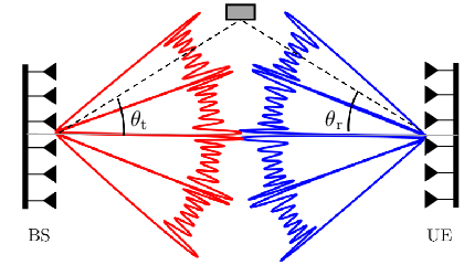
The BS and UE are equipped with uniform linear arrays (ULAs) with $M_{\mathrm{t}}$ and $M_{\mathrm{r}}$ antenna elements, respectively, and use analog beamforming. The signal received at the UE is

where $P_{\mathrm{tx,k}}$ is the average transmit power of the BS; $\mathbf{s}\in\mathbb{C}^{S}$ is the transmitted signal with $S$ symbols with $\Exp[\lVert\mathbf{s}\rVert_{2}^{2}]={S}$; $\mathbf{H}_{k}{\in}\mathbb{C}^{M_{\mathrm{r}}\times M_{\mathrm{t}}}$ is the channel matrix; $\mathbf{v}_{k}{\in}\mathbb{C}^{M_{\mathrm{t}}}$ is the BS beamforming vector with $\|\mathbf{v}_{k}\|_{2}^{2}=1$; $\mathbf{u}_{k}{\in}\mathbb{C}^{M_{\mathrm{r}}}$ is the UE combining vector with $\|\mathbf{u}_{k}\|_{2}^{2}=1$; $\mathbf{w}_{k}{\sim}\mathcal{CN}(\boldsymbol{0},N_{0}W_{\mathrm{tot}}\mathbf{I})$ is additive white Gaussian noise (AWGN), with one-sided power spectral density $N_{0}$ and system bandwidth $W_{\mathrm{tot}}$.
Channel Model: We use the extended Saleh-Valenzuela geometric model with a single-cluster [14], as adopted in several previous works (e.g., see [15, 16, 8]). In fact, typical mm-wave channels have been shown to exhibit one dominant cluster containing most of the signal energy [17]. The single-cluster channel is modeled as

where $\theta_{k}{\triangleq}(\theta_{\mathrm{r},k},\theta_{\mathrm{t},k}){\in}[-\frac{\pi}{2},\frac{\pi}{2}]^{2}$ is the angle of arrival (AoA) and angle of departure (AoD) pair associated to the dominant cluster, with complex fading gain $\alpha_{k}$; $\mathbf{a}_{\mathrm{r}}$ and $\mathbf{a}_{\mathrm{t}}$ are the UE and BS array response vectors, respectively, defined as

where $\psi_{\mathrm{x}}{=}\sin\theta_{\mathrm{x}}$, $d_{\mathrm{x}}$ is the antenna spacing, $\lambda{=}c/f_{c}$ is the wavelength at carrier frequency $f_{c}$, $c$ denotes the speed of light. We assume that during the duration of one frame $T_{\mathrm{fr}}$, $\theta_{k}$ remains unchanged, $\theta_{k}{=}\theta$, and $\alpha_{k}$ are i.i.d. Reyleigh fading in each slot with distribution $\alpha_{k}{\sim}\mathcal{CN}(0,\ell(d)^{-1})$, where $\ell(d)$ is the path loss at distance $d$ from the BS. In fact, the AoA-AoD pair change much slower than the channel gain [18].
Codebook structure: In slot $k$, the BS uses the beamforming vector $\mathbf{v}_{k}{\in}\mathcal{V}$ and the UE uses the combining vector $\mathbf{u}_{k}{\in}\mathcal{U}$, from the codebooks $\mathcal{V}$ and $\mathcal{U}$, respectively. We assume a sectored model [8], in which the AoA and AoD spaces are partitioned into sectors of equal beamwidth (as shown in Fig. 1 for the case of four sectors, this model approximates well analog beamforming). Accordingly, let $\mathcal{B}_{\mathrm{r}}(\mathbf{u}){\subseteq}[-\frac{\pi}{2},\frac{\pi}{2}]$ and $\mathcal{B}_{\mathrm{t}}(\mathbf{v}){\subseteq}[-\frac{\pi}{2},\frac{\pi}{2}]$ denote the AoA and AoD supports of the UE combiner and BS beamformer vectors $\mathbf{u}{\in}\mathcal{U}$ and $\mathbf{v}{\in}\mathcal{V}$, respectively, with equal beamwidth $|\mathcal{B}_{\mathrm{r}}(\mathbf{u})|{=}\frac{\pi}{|\mathcal{U}|},{\forall}\mathbf{u}{\in}\mathcal{U}$ and $|\mathcal{B}_{\mathrm{t}}(\mathbf{v})|{=}\frac{\pi}{|\mathcal{V}|},{\forall}\mathbf{v}{\in}\mathcal{V}$, where $|\mathcal{B}|$ denotes the measure $|\mathcal{B}|{\triangleq}\int_{\mathcal{B}}\mathrm{d}x$. We define $\mathcal{B}(\mathbf{u},\mathbf{v}){\triangleq}\mathcal{B}_{\mathrm{r}}(\mathbf{u}){\times}\mathcal{B}_{\mathrm{t}}(\mathbf{v})$ as the joint AoA-AoD support of $(\mathbf{u},\mathbf{v})$. We assume that the angular supports are mutually orthogonal and form a partition of the entire AoA-AoD space $[-\frac{\pi}{2},\frac{\pi}{2}]^{2}$, i.e., $\mathcal{B}(\mathbf{u},\mathbf{v}){\cap}\mathcal{B}(\tilde{\mathbf{u}},\tilde{\mathbf{v}}){=}\emptyset,\forall(\mathbf{u},\mathbf{v}){\neq}(\tilde{\mathbf{u}},\tilde{\mathbf{v}})$ and $\cup_{\mathbf{u}\in\mathcal{U}}\mathcal{B}_{\mathrm{r}}(\mathbf{u}){=}\cup_{\mathbf{v}\in\mathcal{V}}\mathcal{B}_{\mathrm{t}}(\mathbf{v}){=}[-\frac{\pi}{2},\frac{\pi}{2}]$. Let $(\mathbf{u}^{(i)},\mathbf{v}^{(i)}),i\in\mathcal{I}{\triangleq}\{1,2,\ldots,|\mathcal{U}||\mathcal{V}|\}$ be any ordering of combining and beamforming vectors, and $\mathcal{B}^{(i)}\triangleq\mathcal{B}(\mathbf{u}^{(i)},{\mathbf{v}}^{(i)})$ be their support. Let $A_{k}{\in}\mathcal{I}$ be the beam index of the combining and beamforming vectors scanned in slot $k$, so that $(\mathbf{u}_{k},\mathbf{v}_{k}){=}(\mathbf{u}^{(A_{k})},\mathbf{v}^{(A_{k})})$. Let $X$ be a discrete random variable denoting the index of the support that the AoA-AoD pair $\theta$ of the channel belongs to, so that $\theta{\in}\mathcal{B}^{({X})}$. Then, from (1)-(2), the received signal can be expressed as¹¹ 1 The phase of $\mathbf{u}_{k}^{H}\mathbf{a}_{\mathrm{r}}(\theta_{\mathrm{r}})\mathbf{a}_{\mathrm{t}}^{H}(\theta_{\mathrm{t}})\mathbf{v}_{k}$ is incorporated into $\alpha_{k}$.

where $\delta[\cdot]$ is the Kronecker’s delta function, equal to $1$ if alignment is achieved ($A_{k}{=}X$), equal to $0$ otherwise ($A_{k}{\neq}X$); $G$ and $g$ are, respectively, the main and side lobe gains of the sectored model, expressed as

In the following, we describe the beam-alignment and data communication procedures.
Beam-Alignment: In each slot $k$ of the beam-alignment phase, the BS transmits a pilot sequence $\mathbf{s}$ using the beam index $A_{k}$, with transmit power $P_{\mathrm{tx},k}{=}P_{\mathrm{ba}}$. Upon receiving $\mathbf{z}_{k}$ (based on the combining vector with index $A_{k}$), the UE uses a matched filter to compute the signal strength and sends the normalized received power feedback signal $Y_{k}$ back to the BS, of the form

where $\Lambda{\triangleq}\frac{P_{\mathrm{ba}}\|\mathbf{s}\|^{2}}{N_{0}W_{\mathrm{tot}}\ell(d)}$ is the pre-beamforming receive SNR during beam-alignment. Then, the probability density function (pdf) of $Y_{k}$ conditional on $(X,A_{k}){=}(x,a_{\mathrm{s}})$ is given by

where $1/\nu$ is the mean signal power in case of alignment, with

The BS uses a Bayesian approach to select $A_{k}$: starting from $\mathcal{H}_{0}{\triangleq}\emptyset$ and given the history of feedback and scanned beam indices $\mathcal{H}_{k}{\triangleq}\{(A_{j},Y_{j})\}_{j=0}^{k-1}$, the next beam index $A_{k}$ is selected. This procedure continues until the end of the beam-alignment phase.
Data communication: Upon completion of the beam-alignment phase, given the history of feedback and actions $\mathcal{H}_{L}$, the BS selects the data communication parameters: beam index for data communication $A_{\mathrm{d}}{{\in}\mathcal{I}}$, transmission power $P_{\mathrm{d}}{\in}[0,P_{\max}]$, and data rate $R_{\mathrm{d}}{\geq}0$. These parameters are used until the end of the data communication phase.

Let $b_{0}[x]$ be the prior belief over $X{=}x$ (or equivalently over $\theta{\in}\mathcal{B}^{(x)}$) available at the beginning of the beam-alignment phase. We define the expected rate during the communication phase (normalized by the frame duration), as

where we have defined

The probability term in (II) is the probability of achieving correct alignment, given the prior $b_{0}$ and the history $\mathcal{H}_{L}$ of feedback and actions during the beam-alignment phase, whereas the probability term in (8) denotes the probability of non-outage with respect to the realization of the fading process (i.i.d. over time), given that correct alignment has been achieved (we assume that mis-alignment yields outage with probability one, since $g\ll G$).

We now formulate the beam-alignment and data communication problem in the context of a decision process. We define a policy $\mu$, part of our design, which operates as follows. At time $k$ during beam-alignment, given the history of feedback and actions $\mathcal{H}_{k}$, the BS selects the beam-alignment action $A_{k}{=}a_{\mathrm{s}}{\in}\mathcal{I}$ with probability $\mu_{k}(a_{\mathrm{s}}|\mathcal{H}_{k})$; given $\mathcal{H}_{L}$, the BS selects the data communication parameters as $(A_{\mathrm{d}},P_{\mathrm{d}},R_{\mathrm{d}})=\mu_{\mathrm{d}}(\mathcal{H}_{L})$. The goal is to design $\mu$ so as to maximize the expected communication rate, i.e.,

where the expectation $\mathbb{E}_{\mu}$ is conditional on the prior belief $b_{0}$ and on the policy $\mu$ being executed during beam-alignment and data communication. Note that, using (II), we can rewrite the optimization problem as

i.e., the problem can be decomposed into the following two independent problems: 1) find the optimal rate and power $(R_{d}^{*},P_{d}^{*})$ that maximize the expected rate in the communication phase, conditional on correct alignment being achieved ($X{=}A_{\mathrm{d}}$); 2) find the optimal beam-alignment policy and the beam index for communication $A_{\mathrm{d}}$ so as to maximize the probability of correct alignment. The first problem can be solved efficiently by maximizing (8). In the sequel, we consider the latter problem.

Let $b_{k}[x]{\triangleq}\mathbb{P}(X=x|\mathcal{H}_{k},b_{0})$ be the belief over $X{=}x$ given the history of actions and feedback and prior belief $b_{0}$. It serves as a sufficient statistic for optimal control for problem P1. In the following lemma, we present an equivalent simplified sufficient statistic along with its dynamics.

Let $\mathbf{m}_{k}\triangleq[m_{k}[1],\ldots m_{k}[{|\mathcal{I}|}]$. Then, the previous lemma demonstrates that $\mathbf{m}_{k}$ is a sufficient statistic for control decisions, since it is sufficient for computing the belief $b_{k}$ at time $k$. Therefore, $\mu$ can be expressed as $A_{k}=\mu_{k}(\mathbf{m}_{k}),\ \forall 0\leq k\leq L$, which maps the current preference vector $\mathbf{m}_{k}$ to beam index $A_{k}\in\mathcal{I}$. This result makes it possible to achieve an efficient implementation, since the belief can be updated according to simple preference update rules as in (10), rather than via complex Bayesian belief updates. In the subsequent analysis, we will use $\mathbf{m}_{k}$ rather than $b_{k}$ as the state.

In this section, we evaluate the performance of the second-best beam index selection scheme ($a_{\mathrm{s}}{=}x_{[2]}$) with analog beamforming, and compare it with three other schemes. The first one is based on LTS, a popular MAB scheme [12]. In LTS, at each slot the action is chosen according to the belief distribution, i.e., $a_{\mathrm{s}}{\sim}b[x]$. The second scheme is based on scanning the most-likely beam index ($a_{\mathrm{s}}{=}x_{[1]}$) as proposed in [10] (first-best). The third scheme is based on UCB as proposed in [9]. We evaluate the performance of these three schemes in terms of the probability of alignment and spectral efficiency using Monte-Carlo simulation with $10^{5}$ iterations for each simulated point, with parameters as follows: $M_{\mathrm{t}}{=}128$, $M_{\mathrm{r}}{=}1$, $N_{0}{=}{-}174\mathrm{dBm/Hz}$, $W_{\mathrm{tot}}{=}200\mathrm{MHz}$, $T_{\mathrm{fr}}{=}20\mathrm{ms}$, $T_{s}{=}0.1\mathrm{ms}$, $f_{c}{=}30\mathrm{GHz}$, $d{=}10$m, $[\text{path loss exponent}]{=}2$. The BS uses $M_{\mathrm{t}}{=}128$ antennas and partitions the AoD space into $32$ sectors, each with a beamwidth of $\pi/32\mathrm{rad}$ and with uniform prior $b_{0}[x]=1/32,\ \forall x\in\mathcal{I}$; the UE is isotropic, hence it uses $M_{\mathrm{r}}{=}1$ antenna with a single sector. We use the beamforming design proposed in [13] for ULAs with antenna spacing $d_{\mathrm{t}}{=}\lambda/2$. With this configuration, the main-lobe and side-lobe gains are best approximated by $G\approx 14\mathrm{dB}$, $g\approx-11\mathrm{dB}$.

In Fig. 2, we depict the probability of alignment achieved by the aforementioned schemes versus the pre-beamforming SNR $\Lambda$. It can be observed that second-best has better performance than the other three schemes, with up to 7%, 10%, and 30% performance gains compared to first-best, LTS-based and UCB-based schemes. The performance gain of second-best is attributed to a better exploration-exploitation trade-off. The first-best scheme suffers from poor exploration since it ”greedily” chooses the beam index most likely to succeed, but fails to test other beams that may be under-explored, and is thus prone to make alignment errors. On the other hand, LTS-based scheme suffers from poor exploitation since it may scan least likely beams. The proposed second-best scheme, on the other hand, strikes a favorable trade-off between exploration and exploitation: instead of greedily choosing the most likely beam, it chooses the second most likely one, leading to better exploration than first-best; simultaneously, by not choosing beam pairs that are unlikely to succeed, it leads to a better exploitation compared to the LTS-based and UCB-based schemes. Finally, compared to UCB, second-best is better tailored to the structure of the model, since it aims to maximize the alignment probability at the end of the beam-alignment phase (see (16)), rather than the surrogate metric of UCB – the cumulative SNR accrued during beam-alignment.

In Fig. 3, we depict the spectral efficiency against the fraction of $T_{\mathrm{fr}}$ used for BA $LT_{\mathrm{s}}/T_{\mathrm{fr}}$. We fix the SNR for beam-alignment as $\Lambda=0\mathrm{dB}$ and the data-communication power as $P_{\mathrm{d}}^{*}{=}22\mathrm{dBm}$. Similar to Fig. 2, second-best outperforms the three other schemes, owing to improved alignment. The spectral efficiency is maximized at a unique maximizer $L^{*}$: it increases initially with $L{\leq}L^{*}$ as the beam-alignment probability improves with $L$. However, as $L$ increases beyond $L^{*}$, this gain is offset by the increased overhead and reduced duration of the data communication phase.

In this paper, we have formulated the beam-alignment problem as a Bayesian MAB problem. For the optimal control design, we have identified a simplified sufficient statistic referred to as the preference of beam pairs. Based on the preference and bounding of the value function, we have proposed a heuristic policy, which selects the beam pair with the second best-preference to scan. We have shown numerically that the proposed scheme outperforms the first-best, LTS, and UCB based beam-alignment schemes proposed in the literature.

References

- [1] M. R. Akdeniz, Y. Liu, M. K. Samimi, S. Sun, S. Rangan, T. S. Rappaport, and E. Erkip, “Millimeter Wave Channel Modeling and Cellular Capacity Evaluation,” IEEE Journal on Selected Areas in Communications, vol. 32, no. 6, pp. 1164–1179, June 2014.
- [2] T. S. Rappaport, R. W. Heath, R. C. Daniels, and J. N. Murdock, Millimeter wave wireless communications. Prentice Hall, 2015.
- [3] C. Jeong, J. Park, and H. Yu, “Random access in millimeter-wave beamforming cellular networks: issues and approaches,” IEEE Communications Magazine, vol. 53, no. 1, pp. 180–185, January 2015.
- [4] V. Desai, L. Krzymien, P. Sartori, W. Xiao, A. Soong, and A. Alkhateeb, “Initial beamforming for mmWave communications,” in 48th Asilomar Conference on Signals, Systems and Computers, Nov 2014.
- [5] M. Hussain and N. Michelusi, “Throughput optimal beam alignment in millimeter wave networks,” in 2017 Information Theory and Applications Workshop (ITA), Feb 2017, pp. 1–6.
- [6] R. A. Hassan and N. Michelusi, “Multi-user beam-alignment for millimeter-wave networks,” in 2018 Information Theory and Applications Workshop (ITA), Feb 2018, pp. 1–6.
- [7] N. Michelusi and M. Hussain, “Optimal beam-sweeping and communication in mobile millimeter-wave networks,” in 2018 IEEE International Conference on Communications (ICC), May 2018, pp. 1–6.
- [8] M. Hussain and N. Michelusi, “Energy-efficient interactive beam alignment for millimeter-wave networks,” IEEE Transactions on Wireless Communications, vol. 18, no. 2, pp. 838–851, Feb 2019.
- [9] M. Hashemi, A. Sabharwal, C. Emre Koksal, and N. B. Shroff, “Efficient beam alignment in millimeter wave systems using contextual bandits,” in IEEE INFOCOM 2018, April 2018, pp. 2393–2401.
- [10] S. Chiu, N. Ronquillo, and T. Javidi, “Active learning and CSI acquisition for mmwave initial alignment,” IEEE Journal on Selected Areas in Communications, 2019, to appear. [Online]. Available: http://arxiv.org/abs/1812.07722
- [11] M. Hussain and N. Michelusi, “Coded Energy-Efficient Beam-Alignment for Millimeter-Wave Networks,” in 56th Annual Allerton Conference on Communication, Control, and Computing (Allerton), Oct 2018, pp. 407–412.
- [12] A. G. Sutton, Richard S. Barto, Reinforcement learning: An introduction. MIT Press, 2018.
- [13] S. Noh, M. D. Zoltowski, and D. J. Love, “Multi-Resolution Codebook and Adaptive Beamforming Sequence Design for Millimeter Wave Beam Alignment,” IEEE Transactions on Wireless Communications, vol. 16, no. 9, pp. 5689–5701, Sep. 2017.
- [14] A. A. M. Saleh and R. Valenzuela, “A statistical model for indoor multipath propagation,” IEEE Journal on Selected Areas in Communications, vol. 5, no. 2, pp. 128–137, February 1987.
- [15] C. N. Barati, S. A. Hosseini, M. Mezzavilla, T. Korakis, S. S. Panwar, S. Rangan, and M. Zorzi, “Initial Access in Millimeter Wave Cellular Systems,” IEEE Transactions on Wireless Communications, vol. 15, no. 12, pp. 7926–7940, Dec 2016.
- [16] Y. Li, J. G. Andrews, F. Baccelli, T. D. Novlan, and C. J. Zhang, “Design and analysis of initial access in millimeter wave cellular networks,” IEEE Transactions on Wireless Communications, vol. 16, no. 10, pp. 6409–6425, Oct 2017.
- [17] M. R. Akdeniz, Y. Liu, M. K. Samimi, S. Sun, S. Rangan, T. S. Rappaport, and E. Erkip, “Millimeter wave channel modeling and cellular capacity evaluation,” IEEE Journal on Selected Areas in Communications, vol. 32, no. 6, pp. 1164–1179, June 2014.
- [18] V. Va, J. Choi, and R. W. Heath, “The impact of beamwidth on temporal channel variation in vehicular channels and its implications,” IEEE Transactions on Vehicular Technology, vol. 66, no. 6, pp. 5014–5029, June 2017.