Star-forming clumps in the Lyman Alpha Reference Sample of galaxies - I. Photometric analysis and clumpiness2019Star-forming clumps in the Lyman Alpha Reference Sample of galaxies - I. Photometric analysis and clumpiness–11
Abstract
We study young star-forming clumps on physical scales of pc in the Lyman-Alpha Reference Sample (LARS), a collection of low-redshift () UV-selected star-forming galaxies. In each of the 14 galaxies of the sample, we detect clumps for which we derive sizes and magnitudes in 5 -optical filters. The final sample includes clumps, of which have magnitude uncertainties below 0.3 in all filters. The luminosity function for the total sample of clumps is described by a power-law with slope . Clumps in the LARS galaxies have on average values higher than what observed in HII regions of local galaxies and comparable to typical SFR densities of clumps in galaxies. We derive the clumpiness as the relative contribution from clumps to the emission of each galaxy, and study it as a function of galactic-scale properties, i.e. and the ratio between rotational and dispersion velocities of the gas (). We find that in galaxies with higher or lower , clumps dominate the emission of their host systems. All LARS galaxies with Ly escape fractions larger than have more than of the luminosity from clumps. We tested the robustness of these results against the effect of different physical resolutions. At low resolution, the measured clumpiness appears more elevated than if we could resolve clumps down to single clusters. This effect is small in the redshift range covered by LARS, thus our results are not driven by the physical resolution.
Keywords:
galaxies – galaxies: starburst – galaxies: star clusters – galaxies: star formation1 Introduction
High-redshift () star-forming galaxies are morphologically dominated by clumpy structures (Cowie et al. 1995; van den Bergh et al. 1996) which can account for of the galactic rest-frame emission (Elmegreen et al. 2005, e.g.). Such star-forming clumps have observed sizes kpc and estimated masses (Elmegreen et al. 2007; Guo et al. 2012; Tacconi et al. 2013). Their surface densities are times the disk density and many of them form stars at high rate (, Förster Schreiber et al. 2011; Genzel et al. 2011). These characteristics make them very different to the ‘moderate’ star-forming regions observed in the local universe. The difference must be set by the specific conditions of galaxies at high redshift: the majority of high-redshift galaxies show signs of rotation, indicating the presence of disks (Genzel et al. 2006; Förster Schreiber et al. 2006; Shapiro et al. 2008), which have been observed to be highly turbulent (Cresci et al. 2009; Förster Schreiber et al. 2009; Wisnioski et al. 2015) and with gas-to-stellar mass ratios times higher than in local disks (Tacconi et al. 2008; Tacconi et al. 2013; Saintonge et al. 2013). The standard interpretation is that giant clumps are the result of gas collapse due to gravitational instabilities in the disk, which at high redshift can fragment at much larger scales because of its aforementioned properties (Elmegreen et al. 2009; Tamburello et al. 2015, e.g.).
Recent studies on lensed galaxies have allowed the analysis of high-redshift galaxies down to pc resolution (Livermore et al. 2012; Adamo et al. 2013; Wuyts et al. 2014; Cava et al. 2018, e.g.) revealing that clumps are on average smaller and less massive () than previously thought. However, there are indications that clump properties evolve with redshift (Livermore et al. 2015).
Massive clumps shape the morphologies of galaxies and possibly affect their evolution in the systems we observe locally. It is still not clear what are the time-scales for clump survival in their host galaxies. High-redshift clumps have usually estimated ages around Myr, which can reach up to Gyr (Guo et al. 2012, e.g.). Models of clump evolution proposed that they can slowly migrate towards the centre of the galaxy, where they will eventually coalesce, contributing to the formation of the galactic bulge and of the thick disk (Bournaud et al. 2007; Elmegreen 2008). Observations of single galaxies seem to support this scenario (Guo et al. 2012; Adamo et al. 2013; Cava et al. 2018, e.g.) but in general the test of such models is limited by the need for a thorough characterization of both clump properties and their position in the galaxy.
Feedback from young clumps can also affect the evolution of galaxies, as it is responsible for the suppression of global star formation and for the formation of a multi-phase interstellar medium (ISM) (Hopkins et al. 2012; Goldbaum et al. 2016, e.g.). The impact of stellar feedback from clusters and clumps on galaxies can be so great that it may facilitate the escape of UV radiation into the inter-galactic medium (Bik et al. 2015; Bik et al. 2018, e.g.). For this reason, understanding the feedback process is fundamental to understand the escape of radiation from galaxies at high redshift and the reionisation of the universe (Bouwens et al. 2015). Despite having such a big effect on the galaxy and its surroundings, the escape of UV radiation is possible only after clearing the dense clouds surrounding the very young star clusters (Dale 2015; Howard et al. 2018). Both the escape of ionizing radiation and that of resonant lines (e.g. Ly) strongly depend on the gas distribution and conditions at sub-galactic scales.
The study of local galaxies with properties resembling the ones at high redshift allows the exploration of physical scales impossible to resolve in more distant galaxies and therefore help the understanding of what regulates the star formation process. As an example, Fisher et al. 2017a were able to study star-forming clumps on scales pc in the DYNAMO sample (Green et al. 2014), a collection of galaxies at with high gas fractions (, where , Fisher et al. 2014) and H velocity dispersions km/s (Green et al. 2014; Bassett et al. 2014), similar to those of high-redshift turbulent, clumpy disks. Due to the good characterisation of the clumps, the study of the DYNAMO sample was able to support the instability models describing star-formation at high redshift and in particular that the galaxy clumpiness is related to the ratio of velocity dispersion to rotation velocity (Fisher et al. 2017a; Fisher et al. 2017b).
The Lyman-Alpha Reference Sample (LARS) is a galaxy sample consisting of 14 low-redshift starburst systems () observed in multiple bands with the Hubble Space Telescope (HST) in order to study resolved Ly emission from low-redshift galaxies (Hayes et al. 2014; Östlin et al. 2014). The galaxies are characterized in the filters by star-forming clumps, which, due to the proximity of the galaxies, are resolved down to much smaller spatial scales ( pc) than the high-redshift systems. These observations can therefore help fill the gap between the star clusters studied in local galaxies (clusters have typical sizes pc) and the more massive clumps observed in more distant galaxies (studied on scales pc). The different morphological (Östlin et al. 2014; Guaita et al. 2015; Micheva et al. 2018) and kinematic (Herenz et al. 2016) properties of the LARS galaxies can be used to test the clumpiness against the properties of the host galaxies. We divide the study of star-forming clumps in LARS galaxies in two parts: in this present work we study the photometric properties of the clumps, with the goal of understanding what affects the typical luminosities and surface brightnesses of clumps, as well as the clumpiness of the galaxies themselves. In a second work (Messa et al., in prep) we study physical properties (ages, masses, extinctions) of clumps, derived via broadband SED fitting, and study the ionizing budget of clumps, comparing it to the observations of Ly and H maps. This paper is divided as following: in Section 2 we describe the sample selection, observation and some derived properties of the LARS sample, briefly summarizing previous works of the LARS collaboration. In Section 3 we describe the extraction of the clump catalogue and its photometric analysis. In Section 4 we present the results of the analysis. Finally, the main analyses and findings of this work are summarized in the conclusions, Section 5.
2 Sample of study and observations
The galaxies used in this study constitute the Lyman-Alpha Reference Sample (LARS), whose properties and selection are extensively described in Östlin et al. 2014. We report here a summary of the sample selection, observations and main galaxy properties.
2.1 Sample selection
LARS is a sample of 14 galaxies in the low-redshift universe, with redshifts spanning the range . They were selected from a cross-match between SDSS(DR6) and (DR3) catalogues as star-forming galaxies, with EW(H Å. It was found that this criterion leads to samples dominated by compact systems, mainly of irregular morphology (Heckman et al. 2005), whereas lowering the EW(H) limit would favour the inclusion of more ordinary-looking disk galaxies. Galaxies with strong active galactic nuclei (AGN) were rejected by selecting galaxies with narrow H line widths (line-of-sight km/s) and based on their position on the BPT diagram (Baldwin et al. 1981). In selecting the targets following these two main criteria, an effort was made to cover a wide range of FUV luminosities and priority was given to low-z galaxies (in order to better characterize sub-galactic scales) and to galaxies with HST archival data. The selected sample of 14 galaxies is listed in Tab 1, together with their main properties derived by SDSS and . They span a FUV luminosity range between and , which encompasses that of high-z Lyman- emitters (Nilsson et al. 2009, LAEs, e.g.), selected LAEs (Deharveng et al. 2008), and selected Lyman-break galaxy (LBG) analogues (Hoopes et al. 2007; Overzier et al. 2008).
| ID | z | W(H) | O/H | O/HO3N2 | ||||||||
|---|---|---|---|---|---|---|---|---|---|---|---|---|
| (Å) | (kpc) | () | () | () | (km/s) | |||||||
| (1) | (2) | (3) | (4) | (5) | (6) | (7) | (8) | (9) | (10) | (11) | (12) | |
| 01 | 0.028 | 575 | 9.92 | |||||||||
| 02 | 0.030 | 315 | 9.48 | |||||||||
| 03 | 0.031 | 241 | 9.52 | |||||||||
| 04 | 0.033 | 237 | 9.93 | |||||||||
| 05 | 0.034 | 340 | 10.01 | |||||||||
| 06 | 0.034 | 464 | 9.20 | |||||||||
| 07 | 0.038 | 434 | 9.75 | |||||||||
| 08 | 0.038 | 170 | 10.15 | |||||||||
| 09 | 0.047 | 522 | 10.46 | |||||||||
| 10 | 0.057 | 100 | 9.74 | |||||||||
| 11 | 0.084 | 108 | 10.70 | |||||||||
| 12 | 0.102 | 447 | 10.53 | |||||||||
| 13 | 0.147 | 226 | 10.60 | |||||||||
| 14 | 0.181 | 605 | 10.69 |
2.2 HST observations
LARS galaxies were imaged using multi-band observations with HST. The filters were chosen to be able to characterize emission from stellar continuum as well as from H, H and Ly lines. H and H were observed via narrowband filters. Emission from Ly was imaged using a synthetic filter made from the combination of long-pass filters of the solar-blind channel (SBC) camera, F125LP and F140LP for LARS01 to LARS12 and F140LP and F150LP for LARS13 and LARS14. The stellar continuum was sampled near the Ly line with the F150LP filter and on both sides of the 4000 Å break in and bands (Hayes et al. 2009). This filter combination allows us to derive ages and masses for the stellar component of the galaxy via broadband SED fitting. In order to obtain a better accuracy in the SED fit, a filter at redder wavelengths is also included ( band). A typical filter set for LARS observations consist therefore of ACS11 1 ACS: Advanced Camera for Surveys./SBC F125LP, F140LP and F150LP, WFC322 2 WFC3: Wide Field Camera 3./UVIS F336W, F438W, F775W, F502N and F673N. This is, for example, the set of filters used for observing all LARS galaxies between LARS01 and LARS12, excluding LARS03. Even though no conversion is applied to the Johnsons-Cousins filter system, for the reminder of the paper we keep the same nomenclature, due to the similarity of the central wavelength between that system and our data, in particular referring to F336W, F438W, F775W filters as , and band respectively. A complete list of filter sets and exposure times for the LARS observations is given in Tab. 4 of Östlin et al. 2014. LARS13 and LARS14 count one filter less than the other galaxies, since observations in the F125LP filter were not necessary. The LARS galaxies as observed in the F140LP filter (corresponding to rest-frame wavelength Å) are shown in Fig. 1. All data were drizzled to the same pixel scale of arcsec/pixel.


2.3 Ancillary observations
In order to characterize the ISM inside and around the LARS galaxies, the sample was observed in different wavelength ranges with other facilities, such as the 100-m Green Bank Telescope (GBT) and the Karl G. Jansky Very Large Array (VLA) to spectroscopically study the HI emission from the neutral gas (Pardy et al. 2014) and the Potsdam Multi-Aperture Spectrophotometer (PMAS) to study resolved H kinematics (Herenz et al. 2016). The HI observations available are on much larger scales ( times) than the size of the galaxies themselves and are therefore characterizing the properties of the neutral gas surrounding the galaxies. On the other hand, PMAS observation have spatial resolution around (equivalent to kpc in the closest galaxy and to kpc in the furthest one) and allowed a sub-galactic analysis of LARS galaxies. Details of the observations, data reduction and data analysis of the PMAS data are given in Herenz et al. 2016 and we report here only the derived global properties of the H kinematics, in order to use them to characterize the galaxies in the analyses of this current work. Values of these global properties are listed in Tab. 1. In more detail, the shearing velocity, , which measures large-scale gas bulk motions along the line of sight, was calculated considering the minimum and maximum velocities of H, via , without inclination corrections. The second global property derived is the intrinsic velocity dispersion, , which measures the strength of random motions of the ionized gas. It is derived as the flux-weighted average of the velocity dispersion in each spaxel in the galaxy. Combining these two parameters we can use the ratio as a quantification of whether the gas kinematic is dominated by ordered or turbulent motions. Usually galaxies with are considered dispersion-dominated systems. We point out that high values of do not necessarily imply the presence of rotating disks.
2.4 Summary of the LARS derived properties
The main goal of the LARS project is the study of geometrically resolved Ly emission from star-forming galaxies. To accomplish this, the broad and narrow-band observations are used to fit the stellar and nebular content of the galaxy. Once the contribution of the stellar continuum in the bluest FUV filter is derived and subtracted, the observation in that same filter is used to image the Ly emission of the galaxy.
In order to do so, the frames in various filter are reduced, aligned and PSF-matched (i.e. all are convolved in order to have the same synthetic PSF). The method is explained in detail in Melinder et al. (in prep), where an updated analysis of the LARS galaxies, together with the extension of the project (eLARS) consisting of 28 additional galaxies, will be given. As by-products of the SED fitting we produce maps of some important properties of the galaxies, such as H (continuum subtracted) maps and stellar masses. An overview of these properties for the LARS and eLARS samples are given in Hayes et al. 2014 and Melinder et al. (in prep). We describe here some of the properties derived in the analysis of Melinder et al. (in prep), which will be used in this work.
First of all, since we want to consider global properties, we need to define the physical extent of each galaxy. The extension of the galaxy was measured on the FUV continuum images, binned using a Voronoi tessellation algorithm in order to maintain sufficient signal-to-noise in the outskirts. We define the area over which we measure global properties by including all spatial bins with fluxes greater than the isophotal level that encompass of the FUV continuum flux. In this way the clumps are included in the considered region while high-flux noise peaks outside the galaxies are neglected. The star formation rate (SFR) of the galaxy is derived by summing the FUV continuum flux (extinction corrected) emission inside the galaxy area and using the Kennicutt & Evans 2012 conversion. Stellar mass maps comes from the SED fitting of the Voronoi tessellated maps of the galaxies, where two simple stellar populations (an old one and a young one) are modelled. The mass of both are summed inside the galaxy area. Radii, SFRs and stellar masses, are listed in Tab. 1. The radius reported on the table correspond to one of a circularized region with the same surface as the area of the galaxy we are considering (). We list in the last column of Tab. 1 the values for the escape fractions of Ly radiation, (Ly). In order to take into account the scattering of Ly away from the galaxy, this is measured in a larger region (optimized to get the highest possible signal-to-noise in Ly) than the one used for SFR and . A detailed description about the calculation of (Ly) is given in Melinder et al. (in prep). Other properties of the LARS galaxies, mainly derived by SDSS data, can be found in Östlin et al. 2014.
2.5 Comparison to other low and high-redshift samples
The LARS galaxies were put in the broader context of other galaxy populations in Östlin et al. 2014 and in Guaita et al. 2015. Reporting the considerations discussed in those works, LARS galaxies can be studied as reference of high-z (2<z<3) star-forming galaxies (e.g. Law et al. 2012). They also have continuum sizes and stellar masses similar to those of local starburst Lyman break analogues at (e.g. Overzier et al. 2009; Overzier et al. 2010). In this current work we will compare the stellar clumps of the LARS galaxies to other samples at different redshift. In particular, another local sample of galaxies used as reference for high-redshift systems is the DYNAMO sample (Green et al. 2014), where stellar clumps have been studied down to physical scales of pc (Fisher et al. 2017a). Differently from our sample, the DYNAMO galaxies used in the Fisher et al. 2017a study have been selected to host disks with significant velocity gradients and large gas velocity dispersions in the outer disk, km/s, resulting in a sample dominated by strong rotators. On the other hand, LARS galaxies were selected on equivalent width and FUV emission, in order to ensure galaxies with recent bursts of star formation, but without imposing any constraint on the galaxy dynamics. The resulting sample is dominated, in the morphology and in the dynamics, by irregular and merging systems (Guaita et al. 2015; Herenz et al. 2016). Because of their irregular morphologies and elevated star formation, LARS galaxies could be analogs of merging systems, like the Antennae, which have been observed to host massive star clusters and cluster complexes (e.g. Whitmore et al. 1999; Wilson et al. 2000).
3 Clump extraction and photometry
We created a catalogue of clumps by running the SExtractor software (Bertin & Arnouts 1996) on each of the galaxies. The -band filter was used as the reference filter for the extraction, as it constitutes a good compromise between the UV, where the young clumps are brightest but the extinction is also the highest, and the longer wavelengths, where the extinction is lower but the clumps are mixed with the older stellar field of the galaxies, which dominates the light at these wavelengths.
When finding the sources with SExtractor we noticed two critical aspects that strongly affect the process. First, LARS galaxies have diffuse light emission of very different surface brightnesses, often caused by their disturbed morphologies, and this requires the ability of extracting clumps located at different background levels. In some cases, the background level changes on scales of a few pixels.
In addition, clumps are often clustered together, with the necessity of high deblending factors. For these reasons, in order to avoid missing sources, for half of the galaxies we ran SExtractor twice, with different input parameters and in particular with different sizes of the rectangular grid inside which local background is estimated (Ba). Other key parameters of the extraction were the threshold signal-to-noise per pixel which defined a detection (), the deblending parameter for nearby sources (Deb, i.e. the minimum flux fraction that the branch of a composite object should have in order to be considered as a separate object) and minimum number of pixels above the threshold (), which was kept fixed at 5 for all the runs. The choice of doing a second run was based on a visual inspection of the extracted sources.
Details of the configuration files used in the extraction are given in Tab. 2. To give an example of how the extraction is sensitive to the these parameters, in LARS01 changing the signal-to-noise requested for a detection from to reduces by almost half the number of extracted sources. Changing the background size has a smaller effect, as, on the same galaxy, doubling background size reduces by the number of extracted sources, while the deblending parameter has even a smaller effect, affecting only less than of the sources.
The extracted catalogue was visually inspected to remove clear interlopers such as bright pixels at the border of the chip and clumps belonging to nearby galaxies in the HST frame (in LARS09 and LARS1133
3
LARS09 and LARS11 have companion galaxies, mainly falling outside the field of view of the SBC.).
| Gal. | Run 1 | Run 2 | ||||||
| L01 | 5 | 3 | 0.005 | 5 | ||||
| L02 | 5 | 3 | 0.005 | 5 | ||||
| L03 | 5 | 4 | 0.001 | 5 | 5 | 4 | 0.001 | 20 |
| L04 | 5 | 4 | 0.001 | 5 | 5 | 4 | 0.001 | 20 |
| L05 | 5 | 4 | 0.001 | 5 | 5 | 4 | 0.001 | 10 |
| L06 | 5 | 2.5 | 0.001 | 20 | 5 | 2.5 | 0.001 | 500 |
| L07 | 5 | 4 | 0.0001 | 5 | ||||
| L08 | 5 | 4 | 0.0001 | 5 | ||||
| L09 | 5 | 4 | 0.001 | 5 | ||||
| L10 | 5 | 4 | 0.001 | 5 | 5 | 4 | 0.001 | 20 |
| L11 | 5 | 4 | 0.001 | 5 | 5 | 4 | 0.001 | 20 |
| L12 | 5 | 3 | 0.001 | 5 | ||||
| L13 | 5 | 3 | 0.001 | 5 | 5 | 3 | 0.001 | 10 |
| L14 | 5 | 3 | 0.005 | 5 | ||||
On each of the extracted sources we performed a photometric analysis on filters F140LP, F150LP and on , and bands (in LARS 13 and 14 the filter F140LP is used for observing the Ly emission and is therefore neglected in the clump photometric analysis). We report here the main steps of the photometric analysis (see Appendix A for further details and the description of a series of tests on completeness and uncertainties). Each source was analysed in a pixel cut-out, large enough to contain most of its flux but avoiding too strong contamination from neighbouring sources. Smaller boxes were tested, but contain too little signal to account for all the free parameters considered in the modelling. The clumps were modelled with a circular EFF-Moffat profile (Elson et al. 1987) of index 1.5 (kept fixed for all sources) and effective radius . The Moffat profile was shown to be the best fit to the light profile of young massive clusters (Elson et al. 1987; Bastian et al. 2013) because of its property of having broad emission wings. Ellipticity was not taken into account as many clumps in LARS galaxies are already well-fitted by circularly symmetric profiles, and it would require two additional free parameters. The Moffat profile was convolved with the instrumental PSF (K) to create a model of the observable source. We point out once more that the PSFs of different filters were matched and therefore K is the same for all filters. In order to account for the presence of diffuse background emission (possibly coming from the diffuse stellar population, neighbouring sources or nebular emission), we added a degree polynomial background (described by the parameters ). The observable model (M) is therefore parametrized as:
| (1) |
where , called core radius is related to the effective radius by 44 4 The effective radius (), or half-light radius, is the radius enclosing half of the source’s flux., and the radial distance is defined as , where are the pixel coordinates and are the source centre coordinates inside the box. and parametrize the flux and the size of the source, respectively (the Moffat profile is normalized via the factor ).
We assume each clump to have the same size in all the bands and we fit the model to the cut-out image (over 7x7 pixels) in the 5 bands simultaneously (4 bands for LARS 13 and 14), keeping the same core radius (and same centre coordinates ) but allowing the other parameters to vary from filter to filter. The best-fit values for the parameters were found by minimizing the residuals of the difference between the observable models and the data. We built a probability function based on the sum of the weighted residuals
| (2) |
where are the data, the weights and the sum is done for all pixels in the five bands . The probability function is used to run a Markov chain Monte Carlo (MCMC) sampling. We used the Python package emcee (Foreman-Mackey et al. 2013), which implements the MCMC sampler from Goodman & Weare 2010, and run 50 walkers, each producing 320-step chains but discarding the first 20 steps from each, for a total of 15000 sampling values for each source. We consider the median value of the distribution of each parameter as its best-fit value. Uncertainties on each parameter were found to be symmetric and we consider half the difference between the 15.8 and 84.2 percentiles of each parameter distribution as its uncertainty. Each walker is an independent series and its starting value was chosen drawing it from a normal distribution centred on the maximum-likelihood value, calculated via a least-square fit using the Python package lmfit, and with a standard deviation equal to of the maximum-likelihood value. Data, best fit models and residuals for an example clump are presented in Fig. 3 .

Due to the limited size of the box used for photometry and to the resolution of our data, we were not able to derive the size of some of the sources, and in particular:
- 1.
Our fitting routine is not sensitive to values smaller than 0.3 pixels (see Appendix A.2). Sources whose recovered is smaller than this value are assumed to have as an upper limit.
- 2.
For sources with larger than 3.5 pixels, the core region of the clump is not entirely enclosed in the fitting box. We could not trust the fit of those sources, which therefore were removed from the catalogue. This cut only affects 117 sources out of 1698 ( of the total) and, by visual inspection, these sources turn out to be mainly artefacts of the diffuse emission.
We convert the best-fit fluxes () in each filter into AB magnitudes () and the flux uncertainties into magnitude uncertainties () via . Finally, not all the sources were detected in all bands. We discarded from the sample all the sources with observed magnitude mag in more than 1 band. This cut reduces the total clump catalogue to 1425 sources, which can have magnitude uncertainties up to mag in some filters. In the analyses of the following sections we also select a sub-sample of sources which are well-detected in all bands. We consider in this high-fidelity () sample only clumps with mag in all 5 bands (4 bands for LARS 13 and 14). The sample includes a total of 608 clumps. This further constraint implies that clumps in the catalogue have magnitudes mag.
3.1 Using ESO 338-IG04 as test bench for different resolutions
In order to assess how loss in spatial resolution within our galaxy redshift range affects our analyses, we consider a nearby galaxy observed with a set of filters similar to the LARS sample and degrade its resolution to simulate its observation at the redshifts of the LARS galaxies. We use the nearby starburst dwarf ESO 338-IG04 (also known as Tololo 1924-416, and hereafter shortened to ESO 338), which hosts a population of young star clusters, with masses up to (Östlin et al. 1998; Östlin et al. 2003; Adamo et al. 2011). ESO 338 is at a measured distance of 37.5 Mpc (Östlin et al. 1998) and was observed with HST in filters F218W, F336W, F439W and F814W of the Wide Field and Planetary Camera 2 (Östlin et al. 1998) and with the ACS camera (Östlin et al. 2009) in filters F122M and F140LP of the SBC (program GO 9470, PI: D.Kunth) and in filters F550M and FR565N of the WFC camera (program GO 10575, PI: G.Östlin). As for the LARS galaxies, all the frames of ESO 338 were reduced, aligned and convolved to have the same hybrid PSF in all filters. The pixel scale for all the frames is , which at the distance of ESO 338 corresponds to pc.
We simulate ESO 338 observations at the distance of LARS01 and LARS14 (the closest and the most distant galaxies of our sample, respectively). LARS01 is at a distance of Mpc and has a PSF with full width at half maximum px, or pc. On the other hand the PSF of LARS14 has a pc (3.2 px).

In order to simulate ESO 338 at different redshifts we convolve the images with the Gaussian kernel that produces a PSF with a FWHM of the correct physical scale (60 and 400 pc). After the convolution, the data frames are also re-binned in order to have a physical pixel scale corresponding to the ones of LARS01 and LARS14. Flux conservation is ensured throughout the steps. The original ESO 338 observation in the F140LP filter and the simulated frames at LARS01 and LARS14 redshifts are shown in Fig. 4. For each of the frames we have repeated the clump extraction and analysis, with the following results:
- •
We extracted 157 sources (cluster candidates) in ESO 338, 2 of which have px and are therefore excluded from the sample. Of the remainder, 139 were detected with magnitudes brighter than mag in more than 3 filters and constitute the final catalogue of the galaxy. We consider this the reference sample for our study as it has a sufficient resolution to contain genuine single clusters.
- •
Out of these, 57 sources were detected with a magnitude uncertainty lower than mag in at least 4 filters and are therefore considered part of the high-fidelity () sub-sample. Differently from the LARS galaxies, the requirements for clumps to be part of the sub-sample are applied to at least 4 filters (instead of requiring 5 filters) because in ESO 338 the F218W data are underexposed, leading to larger uncertainties and non-detections (Östlin et al. 1998, see).
- •
In the simulated ESO 338 at the distance of LARS01, which we will refer to as ESO 388 (L01) hereafter, we extracted 82 sources, 4 of which with px. Using the same criteria as described above, 69 sources are part of the final catalogue and 26 are part of the sub-sample.
- •
In ESO 338 simulated at the LARS14 distance, i.e. ESO 388 (L14), we extract only 6 clumps, all with px. 4 of them make the final catalogue and all 4 meet the requirements for being part of the sample.
The physical resolution greatly affects the analysis of star-forming clumps in the galaxy. At larger distances, associations counting tens of clusters and clumps can only be studied as single sources.
In the following sections we will characterize more in detail this bias, using the sizes and luminosities of the clumps extracted from the different realisations of ESO 388 datasets. All the retrieved properties of ESO 338 clumps used in the following sections are summarized in Tab. 3
| ESO 338 | ESO 338 (L01) | ESO 338 (L14) | |
|---|---|---|---|
| 37.5 | 119.1 | 645.9 | |
4 Results
4.1 Sizes
The recovered size distributions of clumps for all LARS galaxies and for the ESO 338 reference sample are plotted in Fig. 5. Due to our limitations in recovering radii smaller than 0.3 pixels described in the previous section, we have a number of unresolved sources in our sample, which in the figure have been assigned the corresponding to px. There are 166 unresolved sources in the total sample and 37 in the sample. In the closest galaxies the limiting is of the order of 10 pc. The majority of the sources, however, are resolved and span a range that extends up to pc. The median value for the total sample is 58 pc, with 1st and 3rd quartiles at 33 pc and 108 pc (median of 71 pc for the , with quartiles at 39 pc and 122 pc). The ranges of (in pc-scale) corresponding to the range set by the limits at 0.3 px and 3.5 px are listed in Tab. 4 along with the median values of the distributions in each galaxy. The decrease in the number of clumps at larger sizes, observed in most of the galaxies, is, in part, an effect of the lower completeness for those systems, due to their lower surface brightness for a given luminosity (the completeness of the sample is described in Appendix A.6).
The main trend retrieved in the size distributions across the LARS galaxies is the increase in the median clump size with redshift, caused by the decrease in physical resolution. This effect is clear in the analysis of clumps in ESO 338, whose sizes are plotted in the last row of Fig. 5. As summarized in Tab. 3, in the original reference sample of ESO 338 we probe sizes in the range pc and we are therefore able to resolve most of the (single) star clusters. This ability is partially lost in ESO 338 (L01), where only the larger clusters (minimum pc) are probed. In ESO 338 (L14) we only detect a few systems, with minimum detectable effective radius pc, which is larger than the maximum at the original redshift.
In nearby galaxies star cluster sizes have been studied in detail. Their typical size ranges between pc (Lada & Lada 2003; Ryon et al. 2015; Ryon et al. 2017, e.g.) even if the most massive ones (), usually called super star clusters, can extend up to pc (Meurer et al. 1995; Bastian et al. 2013, e.g.). We deduce that the unresolved sources that we are observing in the closest LARS galaxies, with pc, may be dominated by single star clusters, while the majority of the sources detected, in the size range pc are associations of clusters, usually called star cluster complexes (Bastian et al. 2005, e.g.). The test done on the reference sample of ESO 338 reveals that many of these larger ( ) clumpy star-forming regions contain multiple single clusters. Therefore, the difference in the scales studied across the LARS galaxies implies a physical difference. The compact ( pc) sources observed in the closest LARS galaxies are possibly gravitationally bound clusters, able to survive and evolve within the host galaxy. On the other hand, many larger sources are possibly gravitationally unbound structures which will dissolve rapidly. Lacking dynamical information of the clumps we are unable to quantify this difference.
| Gal. | range | med. | |
|---|---|---|---|
| (pc) | (pc) | ||
| L01 | 130 (78) | 42 (48) | |
| L02 | 73 (30) | 46 (50) | |
| L03 | 138 (33) | 49 (57) | |
| L04 | 163 (87) | 33 (40) | |
| L05 | 43 (36) | 41 (48) | |
| L06 | 65 (10) | 66 (54) | |
| L07 | 43 (21) | 65 (76) | |
| L08 | 305 (98) | 53 (78) | |
| L09 | 222 (107) | 69 (90) | |
| L10 | 43 (17) | 106 (111) | |
| L11 | 108 (56) | 187 (205) | |
| L12 | 26 (16) | 102 (116) | |
| L13 | 59 (13) | 206 (158) | |
| L14 | 7 (6) | 164 (232) | |
| TOT | 1425 (608) | 58 (70) |
4.2 Luminosity functions
We study the clump magnitude distribution via the luminosity function. The luminosity function, defined as the number of sources per luminosity interval, , has been extensively explored in the studies of young star clusters and HII regions in nearby galaxies. It is parametrized by a power-law, , whose slope was observed to vary from galaxy to galaxy, spanning the entire range from to (see Larsen 2006, and references therein). Some studies suggest that the slope of the function could be correlated with properties of the host galaxy (Whitmore et al. 2014) or with different environments within single galaxies (Messa et al. 2018a; Messa et al. 2018b). In some galaxies the power-law slope was observed get steeper at brighter magnitudes (Whitmore et al. 1999; Gieles 2010), which is why the luminosity function is sometimes described by a Schechter function, with a exponential cut-off at bright magnitudes (Haas et al. 2008). With few assumptions, the shape of the luminosity function can be used as a proxy for the mass distribution and this makes it a powerful tool in studying clusters. Even if the age-dependent light-to-mass ratio of clusters causes the luminosity function to not necessarily have the same shape as the mass function, if the cluster is a continuous power law with the same index at all ages the luminosity function will be a power law with the exact same index (Gieles 2009).
At larger physical scales, Cook et al. 2016 studied tens of thousands star-forming regions in 258 nearby ( Mpc) galaxies observed with GALEX. Those regions span physical scales between and pc, similar to our sample. For every galaxy a clump luminosity function was derived and the resulting power-law slopes () span a wide range of values, , with a median value . The slopes were studied in function of several galaxy properties but weak correlations were found only with SFR and SFR density ().
A possible evolution of the clumps luminosity function with redshift was explored in Livermore et al. 2012; Livermore et al. 2015, studying HII regions (observed in the H line) of physical scales pc in the redshift range . The authors assumed for the luminosity function a fixed slope of , taken from the mass function slope of giant molecular clouds in Hopkins et al. 2012 simulations, and derived a characteristic truncation luminosity which evolves with redshift, going from L0(H) erg/s at to L0(H) erg/s for clumps.
In the study of the LARS sample we are limited by the small number of sources per galaxy. We therefore build a global luminosity function including all clumps together. With the goal of focusing on the young (i.e. bluer) clumps and of comparing them to studies of star-forming clumps in literature, we chose to study their luminosity in the 1500 Å rest-frame (in detail, using the F140LP filter in all galaxies except LARS 13 and 14, where we used the filter F150LP due to their higher redshift). Critical for the analysis of the luminosity function is the choice of the lower luminosity limit considered, which in turn relies on a good understanding of the magnitude completeness limits. As described in Appendix A.6, LARS galaxies have different completeness levels in the . We chose the value at which completeness goes below as the lower magnitude limit for each galaxy. This limit is then converted into a luminosity and the most conservative value among all galaxies is used as the lower luminosity value for the global function. The value chosen is erg/s which is the completeness limit of LARS11.The lower limits of the LARS galaxies are listed in Tab. 5. The global luminosity function is plotted in Fig. 6(a). We did not include the clumps of LARS13 and LARS 14 from this analysis because the number of clusters hosted in these galaxies is small and the completeness limit is high. In total, there are 74 clumps above the completeness limit chosen.
| L01 | L02 | L03 | L04 | L05 | L06 | |
| 22.0 | 23.0 | 24.0 | 24.0 | 23.0 | 24.0 | |
| 2.44 | 1.11 | 0.49 | 0.54 | 1.38 | 0.59 | |
| 17 | 6 | 5 | 5 | 15 | 3 | |
| 7 | 3 | 1 | 2 | 8 | 1 | |
| L07 | L08 | L09 | L10 | L11 | L12 | |
| 22.0 | 24.0 | 23.0 | 24.0 | 23.0 | 24.0 | |
| 4.34 | 0.82 | 3.15 | 1.64 | 10.08 | 5.76 | |
| 12 | 15 | 24 | 7 | 48 | 14 | |
| 5 | 3 | 11 | 5 | 19 | 9 |
We assume a power-law shape for the luminosity function, , and therefore define the normalized probability of finding a source of luminosity as
| (3) |
Using Bayes’ theorem we know that the posterior distribution function for the slope is
| (4) |
where is the observed luminosity distribution of Fig. 6(a). We sample the posterior distribution of using the emcee package (see Section. 3). The median value of the distribution is . The uncertainties stated are retrieved from the and percentiles of the distribution. The slope is within the range of values found in the sample of Cook et al. 2016 and in the studies of star clusters and HII regions in the local universe. The global luminosity function studied includes clumps that span a wide range in sizes, from to 600 pc, and therefore a wide range of different objects, from clusters to extended star-forming regions. In order to restrict the study of the luminosity function to smaller clumps we re-perform the analysis keeping only the galaxies from LARS01 to LARS09. In this way the largest clumps included have pc. We also notice that these galaxies are the ones hosting the most numerous clump populations. The luminosity function is shown in Fig. 6(b). Note that the lower luminosity limit was re-adapted to the selection, becoming erg/s. There are 102 clumps above this completeness limit. The best-fit value for the slope in this case is , which is consistent within uncertainties with the previous result.
In order to account for the low number statistics and to understand how the scatter of points may be affecting the results of the fit, we take into consideration two additional methods for estimating the uncertainties:
- “Jackknife” method:
-
we remove one of the clumps from the sample and re-fit the luminosity function obtaining a new value for the slope. This is repeated for all the sources and we consider the median and the standard deviation of the resulting distribution of slopes as indicative of the best value and uncertainties.
- Monte Carlo sampling of uncertainties:
-
We re-sample the luminosity of each source from a normal distribution centered on its value and with a standard deviation given by the magnitude uncertainty and we fit the new luminosity function. We repeat this process 1000 times. We consider the median and the standard deviation of the resulting distribution of slopes as indicative of the best value and uncertainties.
In both the cases just mentioned it would be computationally expensive to run the sampling of the posterior distribution, as done previously. We decide therefore to fit the function with a least-squares method. The fitted function in this case is the cumulative one, i.e.:
| (5) |
The results of these two additional methods are reported in Tab.6. In both cases the uncertainties recovered are smaller than the ones found with the sampling of the posterior distribution.
The effect of resolution on luminosities was tested with the ESO 338 sample. As expected, at decreasing resolutions single clusters are merged together and the distribution of derived luminosities is shifted to brighter values (Fig. 7). We derive observed-magnitude completeness limits in for ESO 338 and ESO 338 (L01) in a similar way to what done for the LARS galaxies (see Appendix A.6), retrieving in both cases. This magnitude limit corresponds to limits in luminosity of erg/s for ESO 338 and of erg/s for ESO 338 (L01). We study the luminosity function above the luminosity limit finding a slope for ESO 338. We point out that there are only 18 clumps above the limit. In the case of ESO 338 (L01) only two clumps have luminosities above the completeness limit, implying that most of the sample is affected by incompleteness. We fit the luminosity function of ESO 338 (L01) down to erg/s, where we observe the peak of the luminosity distribution in Fig. 7, finding a slope of . The flattening of the slope, compared to the result at the reference redshift, is therefore caused by incompleteness. A similar flattening in function of decreasing resolution was found in the analysis of the clump mass function in high-redshift galaxies in Dessauges-Zavadsky & Adamo 2018.
As done by Cook et al. 2016, we investigate possible correlations between the luminosity function power-law slope and the SFR surface density of the host galaxy. We again focus on the low-redshift galaxies of the sample (LARS 01 to 09) dividing them into two groups. We use the value of as the boundary for separating the two sub-groups because it results in groups of almost equal numbers of clumps (above the completeness value of erg/s), 44 for the high- sample including LARS01, LARS05 and LARS07, 58 for the low- sample including the rest of the galaxies. We point out that the two groups contain galaxies at various redshifts. The two luminosity functions are plotted in Fig.8, together with the best-fit slope values, and . We recover slopes that differ by , and in particular a shallower slope for the high- sample, consistent with what was found by Cook et al. 2016. This result can be interpreted as follows: galaxies with higher (and therefore higher gas surface density, assuming the Kennicutt 1998 relation between and ) form on average more luminous (and therefore more massive) clumps. An important caveat should be considered: all the LARS galaxies are on average highly star-forming galaxies, with large values of . The range of SFR densities that we are probing is therefore limited, and the comparison to galaxies with lower SFR densities (e.g. the galaxies of the eLARS sample, Melinder et al. (in prep)) could increase the significance of this result. We test the dependence of the slope of the clump luminosity function on other galactic-scale properties, namely on and on the galaxy stellar mass, . In the first case, we divide the galaxies in two samples using , commonly used to separate rotation-dominated galaxies from dispersion-dominated ones. In the second case we use to separate the galaxies in two groups, since this value allow to have a similar number of clumps in the groups. We notice that, in our sample, most of the galaxies with high also have low and small stellar masses. As a consequence, we find that the slope of the clump luminosity function is shallower for low-mass and dispersion dominated galaxies (see Tab. 6).
Assuming that a shallower slope indicates the presence of more massive clumps on average, we can try to put these result in the context of clump formation. As described by Dekel et al. 2009, the standard Toomre theory predicts that the typical clump mass scales with the disk mass of the host galaxy. In the case of LARS galaxies we find the opposite relation: the reason for this discrepancy can be attributed to the fact that the systems we are studying are highly perturbed, with a kinematics that is far from regular disks. We observe that in this case the formation of clumps may be regulated instead by the and parameters.
| Sample | Included | |||
|---|---|---|---|---|
| (1) | (2) | (3) | (4) | (5) |
| 1-12 | ||||
| 1-9 | ||||
| 2,3,4,6,8,9 | ||||
| 1,5,7 | ||||
| low | 2,5,7 | |||
| high | 1,3,4,6,8,9 | |||
| low | 1,2,5,6,7 | |||
| high | 3,4,8,9 |
As a last remark, we find that the luminosity function in the LARS galaxies is described by a simple power-law without the need of a truncation at high luminosities. The reason is likely the low number of clumps available: in order to sample the truncation a large statistical sample above completeness is necessary, usually of several hundreds of sources (Adamo et al. 2017, e.g.), which we are lacking.
4.3 Clumps SFR vs size relation
We convert clumps’ luminosities to SFR values using the relation in Kennicutt & Evans 2012, assuming no intrinsic extinction. In a forthcoming paper, where we analyse the spectral energy distribution of clumps (Messa et al., in prep), we show that the majority of clumps have derived values of extinction mag. In Appendix B.1 we show the effect of considering the extinction values derived in (Messa et al., in prep) on the clumps’ SFR values.
We show the SFR-size plot for our sample in Fig 9(a). We consider both the total sample and the sub-sample, and we notice that the clumps in the latter, at any radius, have on average higher values of SFR. As a consequence, the median /( of the sub-sample is higher than for the total sample, as shown in Fig. 9(a). This suggests, as expected, that the selection of the clumps with low photometric uncertainties implies a bias towards the clumps with higher SFR densities.
We analyse the effect of different redshifts using the clumps in ESO 338, in Fig. 9(b). At increasing simulated redshifts, the sources move towards the top-right corner of the plot, i.e. towards larger sizes and higher SFRs. In doing so, they may change their : the sources in ESO 338 (L01) have a lower median SFR density than their counterparts at reference redshift. Only two sources on ESO 338 (L14) are not upper limits in and they have SFR densities compatible with the median of sources at the original redshift. We notice however that, by degrading the resolution, and therefore studying larger structures, we lose the possibility of characterizing the highest densities. We conclude that the bright single clusters, when studied at larger scales will tend to blend with surrounding sources and have lower observed SFR densities: this result should be kept in mind when comparing clump studies at different redshifts and resolutions. This is consistent with the results of Fisher et al. 2017a, who found that degrading the resolution and sensitivity of local clumps to match the resolutions reached in lensed galaxies has the effect of moving the observed sample to lower values. Part of this difference is caused by the apparent blending of many clumps into a single one, which causes the resulting clump to be brighter and larger in size, thus resulting in smaller (Fisher et al. 2017a, see). A similar conclusion was also reached in Tamburello et al. 2017 by degrading the resolution of H clumps from hydrodynamical simulations of clumpy disk galaxies.
We compare LARS clumps to other samples in literature, taking care to compare clumps of similar physical scales. The SINGS sample (Kennicutt et al. 2003) contains local star forming galaxies (at distances Mpc), with HII regions resolved down to pc size. In Fig. 9c we plot their sizes and luminosities as derived in Wisnioski et al. 2012. In this comparison, it should be noted that SFRs for clumps in SINGS were derived using H observations (via the Kennicutt & Evans 2012 relation), which are associated with slightly different time-scales (H probes on average younger emission than bands) and sizes (H emission is associated to HII regions, while radiation comes directly from the stellar objects). As for our sample, the SFRs of clumps in the SINGS sample were derived without accounting for intrinsic extinction. We notice that the SINGS sample has on average lower SFRs than LARS sample, despite the similar distribution in sizes. This difference points towards a real physical difference in density between the clumps in LARS and SINGS.
Recently, observations have been reported of lensed high-redshift galaxies where extremely compact star-forming regions have been detected, at scales down to pc (Bouwens et al. 2017; Vanzella et al. 2017a; Vanzella et al. 2017b; Vanzella et al. 2019). We take the absolute magnitudes of those samples and convert them into SFR values as done for LARS. Those high-redshift clumps have on average higher values of than clumps in the LARS sample (see Fig.9c); however there is some overlap between the samples, indicating that what was observed at high-redshift can be, as proposed, single star-forming regions or proto-globular clusters, which in some cases are so bright as to outshine the host galaxy. The general difference between the SFR values of clumps in LARS and in those sample is not surprising: as mentioned in Section 2.5, the selection of high-redshift galaxies in Bouwens et al. 2017; Vanzella et al. 2017a; Vanzella et al. 2017b; Vanzella et al. 2019 is biased towards systems with extreme surface brightnesses (small radii and high intrinsic luminosities) that may not be representative of the clump population at z>3.
Livermore et al. 2015 studied the redshift evolution of using samples of H clumps at redshifts from to with sizes pc, suggesting that the mean surface brightness of star forming clumps evolve with redshift as:
| (6) |
We plot in Fig 9(d) the sizes and SFRs of the clumps studied in Livermore et al. 2015, together with their derived average values at redshifts , 1 and 3, and compare them to the clumps with pc in the sub-sample of LARS. In this case, since the SFRs of clumps in the comparison samples were derived taking into account external extinction, we also use for LARS extinction-corrected SFRs, as derived in Appendix B.1. Our sample covers a wide range in SFR densities, extending to much higher values than the predicted average for local galaxies. Most of the LARS clumps are found in the range between and according to the Livermore et al. 2015 prediction. Some clumps have even higher SFR surface densities, reaching the values found for and partially overlapping with local () clumps in the DYNAMO sample of high-redshift galaxies analogues (Fisher et al. 2017a).
We try to understand the origin of this large scatter in clump SFR surface densities. Studying a compilation of H clumps from literature, Cosens et al. 2018 showed that high and low- clumps follow different correlations in the space, possibly suggesting different origins (Strömgren spheres or star forming regions driven by Toomre instability). We divide our clumps sample in a high-SFR surface density ( ) and a low-SFR surface density ( ) sub-samples, similarly to what done in Cosens et al. 2018, and we fit a function of the form . We do not find a difference in the derived slopes in the two sub-samples, with for the high- sub-sample and for the low- sub-sample (see Appendix B.2 for more details on the fit). Both values are close to found for clumps with in Cosens et al. 2018 and close to a relation expected for star forming regions driven by Toomre instability. On the other hand, we observe that the SFR surface density of clumps do depend on the galactic-scale properties of their host galaxies. We divide the galaxies in sub-samples using the same division of Section 4.2 (Tab. 6) and we calculate the median clump SFR surface density in each sub-sample. We find that clumps have on average higher SFR surface density in galaxies characterized by high , low and low (see Appendix B.3 for more details). Similarly to what found in the study if the luminosity function, this result suggests that the galactic-scale properties of the host galaxies affect the clump .
4.4 Clumpiness
Recent studies of the redshift evolution of star-forming regions were motivated by the discovery that galaxies at high redshift appear more clumpy than galaxies in the local universe in the rest-frame (Elmegreen et al. 2009, e.g.). In this section we study the clumpiness of the LARS galaxies as a function of galactic-scale properties. We use two main parametrisations for the clumpiness:
- 1.
Fraction of the galaxy light in clump. This method simply express the clumpiness as the relative contribution of clumps to the galaxy UV emission (Soto et al. 2017, e.g.).
- 2.
Fraction of the galaxy light in the brightest clump. In studying the galaxies of the CANDELS/GOODS-S and UDS fields in the redshift range , Guo et al. 2015 showed that defining clumpy galaxies as those where the brightest (off-centred) clump accounts for at least of the light (rest-frame wavelength in the range Å in their sample) allows to distinguish the high-z star-forming main-sequence galaxies from nearby spirals.
We measure the total rest-frame Å flux of the LARS galaxies inside the regions defined in Section 2.4. In order to estimate clumpiness following method (i), we consider the clumps with pc and sum up their flux. The ratio between the clumps flux and the galactic flux gives the first estimator of clumpiness, that we will call for the rest of the paper. We calculate this ratio considering only clumps in the sub-sample (). The size limit at was imposed to ensure that we are considering clumps at similar scales in all galaxies, as suggested by Johnson et al. 2017. To parametrise clumpiness following method (ii), we considered the flux of the 3rd brightest clump in each galaxy and divide it by the galactic flux (). We consider this measurements more solid than considering the brightest clump within each galaxy, as the latter may correspond with the nuclear region of the galaxy. We present the clumpiness values of the LARS galaxies according to these parametrisations in Tab. 7.
| L01 | |||
|---|---|---|---|
| L02 | |||
| L03 | |||
| L04 | |||
| L05 | |||
| L06 | |||
| L07 | |||
| L08 | |||
| L09 | |||
| L10 | |||
| L11 | |||
| L12 | |||
| L13 | |||
| L14 |
Clumpiness is shown as a function of redshift in Fig. 10. The clumps account for more than of the flux in half of the LARS galaxies. In Fig. 10 we also added the clumpiness of ESO 338 at the three different redshifts considered in this study. The analysis of ESO 338, shows that clumpiness changes by less than going from to and even declines when simulating the galaxy at . Having imposed the restriction of only including clusters with sizes of pc, we avoid the effect of clumpiness increasing as a function of redshift: without this limitation, ESO 338 simulated at would have a clumpiness value of as can be seen in the left panel of Fig. 10. The same figure shows that the values of clumpiness in the LARS galaxies do not show a steady increase with redshift, suggesting that the resolution may be affecting the derived only in the most distant galaxies. The large scatter in the clumpiness values for LARS galaxies in their narrow redshift dynamic range confirms that the specific clumpiness of each galaxy is set by its internal properties more than by its resolution. We test the dependence of the clumpiness measurements on redshift by running a Spearman’s rank correlation test. Correlation coefficients and their associated probabilities (p-values) are collected in the first column of Tab. 8. The coefficients are below 0.2, with high p-values, indicating no correlation.
We notice that LARS galaxies have a higher clumpiness that local galaxies. Larsen & Richtler 2000 measured the fraction of U-band light contributed by young star clusters to the total U-band luminosity of the galaxy in a sample of local galaxies, finding that in spiral galaxies the median fraction is . Even accounting for the increase of observed in ESO338 when going from resolving clusters to clumps, the clumpiness of local spirals is still one order of magnitude below what we observe in the LARS galaxies.
We explore possible correlations of the clumpiness with the galaxy SFR and gas dynamics properties derived in Section 2.4. Specific SFR () and SFR surface density () are derived dividing the -derived SFR by the stellar mass and the galaxy area () respectively. We run a Spearman’s rank correlation test on each combination of clumpiness parametrisation-galaxy property. We note that the number of galaxies in our sample is limited, but we consider the results of the test as indicative of possible correlations. The results of the test are collected in Tab 8.
| redshift | sSFR | (Ly) | ||||
|---|---|---|---|---|---|---|
We observe an anti-correlation between clumpiness and and a positive correlation between clumpiness and the galaxy SFR surface density. The clumpiness shows only a weak correlation with specific SFR (sSFR) and a weak anti-correlation with the galaxy stellar mass, . We show the correlations between and both and in Fig. 11. The high level of scatter and the low number of galaxies in our sample poorly constrain the p-values associated with the correlation coefficients. We can ask ourselves how the correlation coefficient retrieved would change if LARS14 was removed from the sample. As stated before, at the redshift of LARS14 the clumpiness values derived could be affected by the poor physical resolution. Removing the points corresponding to LARS14 data in Fig. 11, the Spearman’s test finds correlation coefficients of and of for the left and the right plots, respectively. The correlation found proves that is not LARS14 alone to drive the derived correlations.
The correlations found in this section were similarly found for the DYNAMO sample in Fisher et al. 2017a, where H clumps were proven to have a higher contribution to the host galaxy emission in galaxies which are more dispersion-dominated (lower ) and have higher sSFR. The DYNAMO sample includes nearby () galaxies with high gas fraction and elevated gas velocity dispersions, resembling the properties of high-redshift galaxies (Fisher et al. 2017a). While in DYNAMO the galaxies hosted a gas-rich rotation-supported disk, the same is not true for the LARS galaxies, which, both from morphological (Guaita et al. 2015) and dynamical (Herenz et al. 2016) studies appear to be mostly merging systems with irregular morphologies (only 2 out of 14 galaxies were classified as rotating disks in Herenz et al. 2016). Fisher et al. 2017b used the clump properties of the DYNAMO sample to validate the disk instability models (Dekel et al. 2009, e.g.) that are expected to regulate star formation at high-redshift. The study of clumps in our sample suggests that, even if the star-formation event is driven by galaxy interactions, the clumpiness is affected by the SFR surface density of the galaxy (which we can consider as a proxy for the gas surface density) and by the rotational-over-dispersion velocity ratio in the gas.
4.4.1 Lyman- escape fraction vs clumpiness
In addition to the galactic-scale properties studied as a function of clumpiness in the previous section, we focus on the relation between clumpiness and the escape of Ly radiation. Clumps are the sources of most of the ionizing radiation (Messa et al. in prep.) and we also know that the escape of Ly radiation from galaxies is very dependent on the gas distribution at sub-galactic scales. We can therefore expect that galaxy morphology and clumpiness have an impact on the amount of Ly radiation escaping. It has been for example suggested that the Ly equivalent width of high redshift galaxies is related to their morphologies and sizes, with compact galaxies having larger equivalent widths compared to galaxies with more extended and diffuse emission or disks (Pentericci et al. 2010; Cowie et al. 2011; Law et al. 2012; Paulino-Afonso et al. 2018). A similar result is found in low-redshift galaxies, where LAEs are found to have more compact morphologies compared to NUV-continuum selected galaxies (Cowie et al. 2010).
Hayes et al. 2014 presented a value of the Ly escape fraction, (Ly), for each of the LARS galaxies. We use updated escape fraction from Melinder et al (in prep.) which are listed in Tab. 1. We ran a Spearman’s rank correlation test between (Ly) and the clumpiness parametrisations described in the previous section, finding, on average, a good correlation, the strongest being with (Tab. 8). We point out again that we have a limited number of galaxies in our sample and therefore the correlation we derive cannot have high statistical significance. When plotting the correlation (Fig. 12), we notice that not all the galaxies with elevated clumpiness have a high fraction of Ly escape. It is instead true that all the galaxies with (Ly) have clumpiness higher than .
The escape fraction of Ly in the LARS galaxies was already studied in previous works and, for example, Herenz et al. 2016 found a hint of anti-correlation between (Ly) and . The anti-correlation, shown in the previous section, between and the clumpiness could therefore predict a clumpiness-(Ly) correlation, consistent with what has been found here.
5 Conclusions
We report on the sizes and luminosity properties of star-forming clumps, in the LARS sample of nearby () galaxies analogues of high-redshift Lyman-break galaxies. The total sample counts 1425 sources, 608 of which have photometric uncertainties smaller than 0.3 mag in the 5 broad bands in which the galaxies are observed. Focusing on the band (rest-frame wavelength Å) we have investigated luminosity distribution, SFRs of the clumps, as well as their contribution to the total emission of the host galaxy, which we refer to as clumpiness. In doing so, we also consider the clumps properties as a function of galactic-scale properties, namely and the ratio between the rotational and dispersion velocity of the galaxy gas (, measured from H observations in Herenz et al. 2016). We obtain the following results:
- 1.
We find clump size between pc, similar to the range found in the literature for clumps in high-redshift galaxies.
- 2.
The luminosity function of the clumps in the LARS galaxies can be described by a power-law with slope , similarly to what has been found in other nearby galaxies (Cook et al. 2016, e.g.). When dividing the clump sample as a function of the host-galaxy , we find that clumps in galaxies with higher SFR density have a shallower luminosity function, i.e. they are on average more luminous (and therefore more massive). The same is true in galaxies with low values of and low stellar masses.
- 3.
Converting the luminosities of clumps into SFR values using Kennicutt & Evans 2012 relation, we study the size-SFR relation of our sample, and compare to other published samples, both local and at high redshift. We find that LARS clumps have on average a higher SFR density than clumps observed in star-forming galaxies. Considering the redshift evolution of of clumps suggested by Livermore et al. 2015, our sample is compatible with SFR density in galaxies at . Some clumps have extreme SFR surface densities, compatible with those found in galaxies at redshift beyond 3. The median SFR surface density of the LARS clumps is higher in galaxies with high , low and low .
- 4.
LARS galaxies have morphologies dominated by clumps. In many galaxies the clump contribution is of the total emission. We find indications of correlation between the clumpiness and SFR surface density and of anti-correlation with .
- 5.
We find moderate positive correlation between the clumpiness and the Ly escape fraction: all the LARS galaxies with (Ly) have clumpiness higher than .
- 6.
In order to account for the resolution effects caused by the different redshifts of galaxies in the LARS sample, we performed the same clump analyses in the nearby galaxy ESO 338-IG04, hosting a population of star clusters at a distance of Mpc. The analyses were repeated degrading the resolution of ESO 338-IG04 in order to simulate its observation at the redshifts of LARS01 and LARS14 (the nearest and the most distant galaxies in the LARS sample). This test shows that degrading the resolution causes the clumps to appear larger and brighter, affecting also the study of clumps SFR surface densities: a better resolution allows the characterisation of star-forming regions with higher . Finally, the galaxies appear more clumpy when imaged at lower resolution. This result should be kept in mind when comparing clumps studied at different scales, especially in high-redshift galaxies, where is usually difficult to constrain sizes lower than pc.
We conclude suggesting that the elevated star-formation conditions of the sample, probably set by mergers and interactions (Guaita et al. 2015; Herenz et al. 2016), can drive the formation of clumps with elevated surface brightnesses, that contribute to a large fraction of the emission of the host galaxies. However, LARS covers a narrow dynamic range in SFRs. In the future, the inclusion of the eLARS sample (Melinder et al., in prep), consisting of galaxies in the same redshift range but with, on average, lower SFRs will help probing the effect of SFR on clumpiness.
Acknowledgements
Based on observations made with the NASA/ESA Hubble Space Telescope, obtained at the Space Telescope Science Institute, which is operated by the Association of Universities for Research in Astronomy, Inc., under NASA contract NAS 5-26555. These observations are associated with program #12310,#11522. The authors gratefully thank Dr. R.Bouwens and Dr. E.Wisnioski for sharing their catalogues. The authors are also thankful to the anonymous referee for comments and suggestions that helped improving the manuscript. A.A., G.Ö. and M.H. acknowledge the support of the Swedish Research Council (Vetenskapsrådet) and the Swedish National Space Agency (SNSA). M.H. acknowledges the continued support as Fellow of the Knut and Alice Wallenberg Foundation.
References
- Adamo et al. (2011) Adamo A., Östlin G., Zackrisson E., 2011, MNRAS, 417, 1904
- Adamo et al. (2013) Adamo A., Östlin G., Bastian N., Zackrisson E., Livermore R. C., Guaita L., 2013, ApJ, 766, 105
- Adamo et al. (2017) Adamo A., et al., 2017, ApJ, 841, 131
- Baldwin et al. (1981) Baldwin J. A., Phillips M. M., Terlevich R., 1981, Publications of the Astronomical Society of the Pacific, 93, 5
- Bassett et al. (2014) Bassett R., et al., 2014, MNRAS, 442, 3206
- Bastian et al. (2005) Bastian N., Gieles M., Efremov Y. N., Lamers H. J. G. L. M., 2005, A&A, 443, 79
- Bastian et al. (2013) Bastian N., Schweizer F., Goudfrooij P., Larsen S. S., Kissler-Patig M., 2013, MNRAS, 431, 1252
- Bertin & Arnouts (1996) Bertin E., Arnouts S., 1996, A&AS, 117, 393
- Bik et al. (2015) Bik A., Östlin G., Hayes M., Adamo A., Melinder J., Amram P., 2015, A&A, 576, L13
- Bik et al. (2018) Bik A., Östlin G., Menacho V., Adamo A., Hayes M., Herenz E. C., Melinder J., 2018, A&A, 619, A131
- Bournaud et al. (2007) Bournaud F., Elmegreen B. G., Elmegreen D. M., 2007, ApJ, 670, 237
- Bouwens et al. (2015) Bouwens R. J., Illingworth G. D., Oesch P. A., Caruana J., Holwerda B., Smit R., Wilkins S., 2015, ApJ, 811, 140
- Bouwens et al. (2017) Bouwens R. J., Illingworth G. D., Oesch P. A., Maseda M., Ribeiro B., Stefanon M., Lam D., 2017, preprint, p. arXiv:1711.02090 (arXiv:1711.02090)
- Cava et al. (2018) Cava A., Schaerer D., Richard J., Pérez-González P. G., Dessauges-Zavadsky M., Mayer L., Tamburello V., 2018, Nature Astronomy, 2, 76
- Cook et al. (2016) Cook D. O., Dale D. A., Lee J. C., Thilker D., Calzetti D., Kennicutt R. C., 2016, MNRAS, 462, 3766
- Cosens et al. (2018) Cosens M., et al., 2018, ApJ, 869, 11
- Cowie et al. (1995) Cowie L. L., Hu E. M., Songaila A., 1995, AJ, 110, 1576
- Cowie et al. (2010) Cowie L. L., Barger A. J., Hu E. M., 2010, ApJ, 711, 928
- Cowie et al. (2011) Cowie L. L., Hu E. M., Songaila A., 2011, ApJ, 735, L38
- Cresci et al. (2009) Cresci G., et al., 2009, ApJ, 697, 115
- Dale (2015) Dale J. E., 2015, New Astron. Rev., 68, 1
- Deharveng et al. (2008) Deharveng J.-M., et al., 2008, ApJ, 680, 1072
- Dekel et al. (2009) Dekel A., Sari R., Ceverino D., 2009, ApJ, 703, 785
- Dessauges-Zavadsky & Adamo (2018) Dessauges-Zavadsky M., Adamo A., 2018, MNRAS, 479, L118
- Elmegreen (2008) Elmegreen B. G., 2008, ApJ, 672, 1006
- Elmegreen et al. (2005) Elmegreen D. M., Elmegreen B. G., Rubin D. S., Schaffer M. A., 2005, ApJ, 631, 85
- Elmegreen et al. (2007) Elmegreen D. M., Elmegreen B. G., Ferguson T., Mullan B., 2007, ApJ, 663, 734
- Elmegreen et al. (2009) Elmegreen D. M., Elmegreen B. G., Marcus M. T., Shahinyan K., Yau A., Petersen M., 2009, ApJ, 701, 306
- Elson et al. (1987) Elson R. A. W., Fall S. M., Freeman K. C., 1987, ApJ, 323, 54
- Fisher et al. (2014) Fisher D. B., et al., 2014, ApJ, 790, L30
- Fisher et al. (2017a) Fisher D. B., et al., 2017a, MNRAS, 464, 491
- Fisher et al. (2017b) Fisher D. B., et al., 2017b, ApJ, 839, L5
- Foreman-Mackey et al. (2013) Foreman-Mackey D., Hogg D. W., Lang D., Goodman J., 2013, PASP, 125, 306
- Förster Schreiber et al. (2006) Förster Schreiber N. M., et al., 2006, ApJ, 645, 1062
- Förster Schreiber et al. (2009) Förster Schreiber N. M., et al., 2009, ApJ, 706, 1364
- Förster Schreiber et al. (2011) Förster Schreiber N. M., et al., 2011, ApJ, 739, 45
- Genzel et al. (2006) Genzel R., et al., 2006, Nature, 442, 786
- Genzel et al. (2011) Genzel R., et al., 2011, ApJ, 733, 101
- Gieles (2009) Gieles M., 2009, MNRAS, 394, 2113
- Gieles (2010) Gieles M., 2010, in Smith B., Higdon J., Higdon S., Bastian N., eds, Astronomical Society of the Pacific Conference Series Vol. 423, Galaxy Wars: Stellar Populations and Star Formation in Interacting Galaxies. p. 123 (arXiv:0908.2974)
- Goldbaum et al. (2016) Goldbaum N. J., Krumholz M. R., Forbes J. C., 2016, ApJ, 827, 28
- Goodman & Weare (2010) Goodman J., Weare J., 2010, Communications in Applied Mathematics and Computational Science, Vol. 5, No. 1, 2010, pp 65–80
- Green et al. (2014) Green A. W., et al., 2014, MNRAS, 437, 1070
- Guaita et al. (2015) Guaita L., et al., 2015, A&A, 576, A51
- Guo et al. (2012) Guo Y., Giavalisco M., Ferguson H. C., Cassata P., Koekemoer A. M., 2012, ApJ, 757, 120
- Guo et al. (2015) Guo Y., et al., 2015, ApJ, 800, 39
- Haas et al. (2008) Haas M. R., Gieles M., Scheepmaker R. A., Larsen S. S., Lamers H. J. G. L. M., 2008, A&A, 487, 937
- Hayes et al. (2009) Hayes M., Östlin G., Mas-Hesse J. M., Kunth D., 2009, AJ, 138, 911
- Hayes et al. (2014) Hayes M., et al., 2014, ApJ, 782, 6
- Heckman et al. (2005) Heckman T. M., et al., 2005, ApJ, 619, L35
- Herenz et al. (2016) Herenz E. C., et al., 2016, A&A, 587, A78
- Hoopes et al. (2007) Hoopes C. G., et al., 2007, The Astrophysical Journal Supplement Series, 173, 441
- Hopkins et al. (2012) Hopkins P. F., Quataert E., Murray N., 2012, MNRAS, 421, 3488
- Howard et al. (2018) Howard C. S., Pudritz R. E., Harris W. E., Klessen R. S., 2018, MNRAS, 475, 3121
- Johnson et al. (2017) Johnson T. L., et al., 2017, ApJ, 843, L21
- Jones et al. (2010) Jones T. A., Swinbank A. M., Ellis R. S., Richard J., Stark D. P., 2010, MNRAS, 404, 1247
- Kennicutt (1998) Kennicutt Robert C. J., 1998, ApJ, 498, 541
- Kennicutt & Evans (2012) Kennicutt R. C., Evans N. J., 2012, Annual Review of Astronomy and Astrophysics, 50, 531
- Kennicutt et al. (2003) Kennicutt Robert C. J., et al., 2003, Publications of the Astronomical Society of the Pacific, 115, 928
- Lada & Lada (2003) Lada C. J., Lada E. A., 2003, ARA&A, 41, 57
- Larsen (2006) Larsen S. S., 2006, Star formation in clusters. p. 35
- Larsen & Richtler (2000) Larsen S. S., Richtler T., 2000, A&A, 354, 836
- Law et al. (2012) Law D. R., Steidel C. C., Shapley A. E., Nagy S. R., Reddy N. A., Erb D. K., 2012, ApJ, 759, 29
- Livermore et al. (2012) Livermore R. C., et al., 2012, MNRAS, 427, 688
- Livermore et al. (2015) Livermore R. C., et al., 2015, MNRAS, 450, 1812
- Messa et al. (2018a) Messa M., et al., 2018a, MNRAS, 473, 996
- Messa et al. (2018b) Messa M., et al., 2018b, MNRAS, 477, 1683
- Meurer et al. (1995) Meurer G. R., Heckman T. M., Leitherer C., Kinney A., Robert C., Garnett D. R., 1995, AJ, 110, 2665
- Micheva et al. (2018) Micheva G., et al., 2018, A&A, 615, A46
- Nilsson et al. (2009) Nilsson K. K., Tapken C., Møller P., Freudling W., Fynbo J. P. U., Meisenheimer K., Laursen P., Östlin G., 2009, A&A, 498, 13
- Östlin et al. (1998) Östlin G., Bergvall N., Roennback J., 1998, A&A, 335, 85
- Östlin et al. (2003) Östlin G., Zackrisson E., Bergvall N., Rönnback J., 2003, A&A, 408, 887
- Östlin et al. (2009) Östlin G., Hayes M., Kunth D., Mas-Hesse J. M., Leitherer C., Petrosian A., Atek H., 2009, AJ, 138, 923
- Östlin et al. (2014) Östlin G., et al., 2014, ApJ, 797, 11
- Overzier et al. (2008) Overzier R. A., et al., 2008, ApJ, 677, 37
- Overzier et al. (2009) Overzier R. A., et al., 2009, ApJ, 706, 203
- Overzier et al. (2010) Overzier R. A., Heckman T. M., Schiminovich D., Basu-Zych A., Gonçalves T., Martin D. C., Rich R. M., 2010, ApJ, 710, 979
- Pardy et al. (2014) Pardy S. A., et al., 2014, ApJ, 794, 101
- Paulino-Afonso et al. (2018) Paulino-Afonso A., et al., 2018, MNRAS, 476, 5479
- Pentericci et al. (2010) Pentericci L., Grazian A., Scarlata C., Fontana A., Castellano M., Giallongo E., Vanzella E., 2010, A&A, 514, A64
- Ryon et al. (2015) Ryon J. E., et al., 2015, MNRAS, 452, 525
- Ryon et al. (2017) Ryon J. E., et al., 2017, ApJ, 841, 92
- Saintonge et al. (2013) Saintonge A., et al., 2013, ApJ, 778, 2
- Shapiro et al. (2008) Shapiro K. L., et al., 2008, ApJ, 682, 231
- Soto et al. (2017) Soto E., et al., 2017, ApJ, 837, 6
- Tacconi et al. (2008) Tacconi L. J., et al., 2008, ApJ, 680, 246
- Tacconi et al. (2013) Tacconi L. J., et al., 2013, ApJ, 768, 74
- Tamburello et al. (2015) Tamburello V., Mayer L., Shen S., Wadsley J., 2015, MNRAS, 453, 2490
- Tamburello et al. (2017) Tamburello V., Rahmati A., Mayer L., Cava A., Dessauges-Zavadsky M., Schaerer D., 2017, MNRAS, 468, 4792
- Vanzella et al. (2017a) Vanzella E., et al., 2017a, MNRAS, 467, 4304
- Vanzella et al. (2017b) Vanzella E., et al., 2017b, ApJ, 842, 47
- Vanzella et al. (2019) Vanzella E., et al., 2019, MNRAS, 483, 3618
- Whitmore et al. (1999) Whitmore B. C., Zhang Q., Leitherer C., Fall S. M., Schweizer F., Miller B. W., 1999, AJ, 118, 1551
- Whitmore et al. (2014) Whitmore B. C., Chandar R., Bowers A. S., Larsen S., Lindsay K., Ansari A., Evans J., 2014, AJ, 147, 78
- Wilson et al. (2000) Wilson C. D., Scoville N., Madden S. C., Charmandaris V., 2000, ApJ, 542, 120
- Wisnioski et al. (2012) Wisnioski E., Glazebrook K., Blake C., Poole G. B., Green A. W., Wyder T., Martin C., 2012, MNRAS, 422, 3339
- Wisnioski et al. (2015) Wisnioski E., et al., 2015, ApJ, 799, 209
- Wuyts et al. (2014) Wuyts E., Rigby J. R., Gladders M. D., Sharon K., 2014, ApJ, 781, 61
- van den Bergh et al. (1996) van den Bergh S., Abraham R. G., Ellis R. S., Tanvir N. R., Santiago B. X., Glazebrook K. G., 1996, AJ, 112, 359
Appendix A Tests of the photometric fitting analysis
We report here additional details and testing of the photometric analysis described in Section 3. The test included in this section are:
- 1.
choice of the box-size for fitting (Section A.1);
- 2.
test of the size resolution (Section A.2);
- 3.
test of the effect of non-detections in some filter (Section A.3);
- 4.
test of the recovered size when considering 5 filters or only the F140LP filter (Section A.4);
- 5.
test of the impact of source subtraction after each source’s fitting (Section A.5);
- 6.
test of the completeness limits of each galaxy (Section A.6).
A.1 Choosing the background and box size
The two major problems encountered in performing the photometric analysis were the crowding of the sources and the contamination from background emission. They put strong constraints on the details of the fitting routine, in particular on the choice of the number of parameters used to model the observation and the fitting radius. We modelled separately the clumps and the background. Clumps were modelled by Moffat profiles convolved with the instrumental PSF. The background was found to change on very small spatial scales. While testing the code we recognized that modelling it with a constant could lead to large errors, even when the area considered for the fit is small. As an example, we show in Fig. 13 the fit of a synthetic source placed in a region of LARS01 with no close neighbouring sources but with a strongly varying background. A fit with a background modelled as a degree polynomial gives a good results, while when the background is modelled as a constant value we retrieve completely wrong values for size and flux. This simple example explains why it is important to accurately model the background. We also found that in such small regions (scales of pixels), considering polynomials of higher degrees does not improve the quality of the fit (while instead increasing the number of free parameters of the fit).
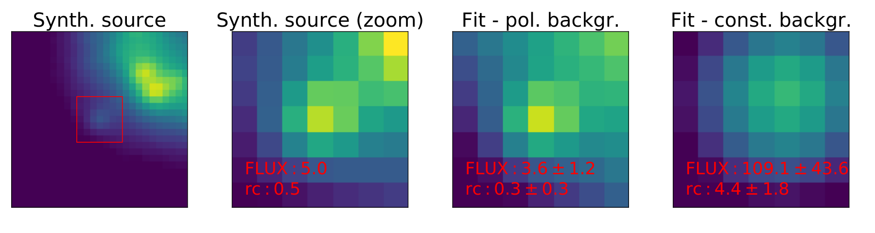
The choice of the number of parameters used for the fit (4 for the clump, 3 for the background) and the sizes of the sources to be fitted strongly influence the choice of the area considered in the fit. We computed the fit in a box region centred on the source, which should be large enough to include the core region of wide sources and whose number of pixels is supposed to be large enough to be able to constrain all free parameters. At the same time the box should be as small as possible in order not to include too much contamination from nearby sources. We performed tests adding synthetic sources of different radii and magnitudes in the band frame of LARS01, and using cut-out boxes of different sizes to fit them. In general, we found that increasing the box area increases the quality of the fit. We decided to consider a px box as the standard dimension for our fitting process because is a good compromise between being able to retrieve the properties of large sources ( px) and not introducing nearby sources in the fit area. For input core radii in the range and input magnitudes between 20 and 25 mag, the fit in the px box results in radii and magnitudes that differ in of the cases by less than 0.14 px and 0.15 mag respectively.
We point out that keeping the same pixel size for the fitting box in all the galaxies implies a different physical scale according to the redshift (7 pixels correspond to 163 pc at the distance of LARS01 but corresponds to pc at the distance of LARS14). The choice was motivated by the ability of characterizing the in the same way across different galaxies. The consequence of studying sources with different physical sizes was already explored in the text in Section 4.1.
A.2 Testing the lowest detectable size
The fitting routine models the observed clump shapes as convolution between the instrumental PSF and a Moffat function of core radius (which parametrizes the intrinsic radius of the source) and for this reason is in principle able to derive infinitely small value. In practice, however, extremely small values are not distinguishable. To test the lowest value that we can confidently distinguish with our code, we simulate synthetic clumps with values uniformly distributed in logarithmic space between and px, putting them at random positions inside LARS01 galaxy and running the photometry code to derive their size. Each filter and was treated independently and only one source at the time was simulated, in order to avoid crowding effects. In total 2500 sources were simulated (500 per filter), with luminosities between 23 and 20 mag. Fig. 14 shows the results of the test: all sources with detected size above 0.3 px have a size difference with the input of less than . Below that value the code starts to be insensitive and the output values are distributed randomly in comparison to the input values. Following the results of this test we assign a value px to all clumps with retrieved values below that value, and treat them as upper limits.
A.3 Non-detection in some of the filters
Clumps were extracted in the band, without requiring a detection in the other filers. For this reason in some cases the photometry routine could be affected by the fact that a source is not detected in some of the 5 bands considered. An incorrect size derivation of the source caused by this non-detection would in turn affect the flux measurement in filters where the source is detected. We tested the effect of non-detections in LARS01 by running the photometry routine a second time on clumps which have a non-detection () in at least one filter. This time photometry is run considering only the filters where the source was detected. A comparison between the fit in all 5 filters and in the detection-filters only is given in Fig. 15.
In most of the cases the derived sizes are the same within the uncertainties. In three cases (out of 20) the two results are incompatible, meaning that the inclusion of all filters have disturbed the fit. For this reason during the analyses of the current paper we selected also a sub-sample of clumps detected in all 5 bands. We point out that most of the source have a non-detection only in one filter out of five.
A.4 Size fit only in the F140LP filter
In our work we derived the size of the clumps using the 5 filters at the same time. This is fundamental because for each clump we want to study the emission from the same region in all filters, in order to be consistent when using the multi-band photometry to fit the broad-band spectral energy distribution (Messa et al., in prep.). Since in this current paper we mostly focused on the clumps emission in the UV band, we tested how the size derivation would be different if only filter F140LP was considered in the size-photometry fit. For this test we used the F140LP map of LARS01 before the convolution to a common PSF. We find that the median difference in the derived core radii is px, with a standard deviation of px. This result suggests that we are not introducing a bias in the size measures (the derived using 5 filters is only px larger, on average). We consider the fit in 5 bands more stable against the background variations and crowding effects. We expect that both these effects are reduced when more than one filter is considered.
A.5 Testing the source subtraction
The photometry routine we developed fits sources starting from the brightest to the least bright, where this ‘preliminary’ brightness was measured in the -band via aperture photometry. After the fit of each source, our routine subtracts its best-fit model (source only, not background) from the science frame, in order to avoid the contamination from the tails of bright sources to the flux of nearby dimmer ones in subsequent fits. To measure the effect of this source subtraction over the derived sizes and magnitudes, we ran on LARS01 a photometric analysis which is identical to the one discussed in the text, except for the fact that clumps fluxes were not subtracted from the science frames after the fitting. Results are given in Tab. 9. The median difference in the recovered values is px, with first and third quartiles of the distribution being px. The difference in values does not depend on the magnitudes, but it affects them. However, the difference in recovered magnitudes in the 5 filters have median values very close to zero. The scatter in the distributions depends on the filter but on average in of the cases are within mag. If only sources in the sub-sample are considered similar results hold. These results assure us that we are not introducing biases in clearing the frames from fitted sources.
| NO SUB WITH SUB | ||
|---|---|---|
| Filter | ||
| F140LP | ||
| F150LP | ||
| F336W | ||
| F438W | ||
| F775W | ||
A.6 Completeness limits
We tested the photometric completeness of the clumps in LARS galaxies filter by filter by inserting synthetic clumps of known properties (sizes and fluxes) in the LARS scientific frames and fitting them with the same photometric code used for the real clumps. For each filter in each galaxy, 1000 synthetic clumps were inserted at random positions inside the area of the galaxy (as defined in Section 4.4), with magnitudes uniformly sampled in the range mag and ˚values sampled from a log-uniform distribution with boundaries px. Sources were inserted and analysed one by one, in order to avoid biasing the results by artificially increasing the crowding. We point out that the source was inserted on top of the science frame and analysed without subtracting possibly brighter sources before the analysis, as was done in the pipeline for the real clumps. In this way the completeness we retrieve is an upper limit, as we know that sources at low luminosities benefit from the subtraction of nearby brighter sources. We show the results of the completeness analysis in Fig. 16. We divide the sample of synthetic sources in bins of 1 mag width and consider as correctly recovered only the sources that satisfy the following conditions:
| (7) |
We find completeness values that vary strongly from galaxy to galaxy, despite similar sets of observations, suggesting that completeness is mainly dependent on properties such as clump crowding and different contribution of galaxy diffuse emission. We report in Tab. 10 for each galaxy and filter the deepest magnitude above a completeness.
| Name | F140LP | F150LP | band | band | band |
|---|---|---|---|---|---|
| mag | mag | mag | mag | mag | |
| L01 | 22 (23) | 22 (23) | 22 (24) | 22 (23) | 22 (23) |
| L02 | 23 (24) | 23 (24) | 23 (25) | 23 (25) | 23 (24) |
| L03 | 24 (25) | 23 (25) | 24 (25) | 23 (24) | 23 (24) |
| L04 | 24 (24) | 23 (24) | 24 (23) | 24 (24) | 23 (24) |
| L05 | 23 (23) | 21 (23) | 23 (24) | 22 (23) | 23 (23) |
| L06 | 24 (25) | 24 (25) | 24 (25) | 24 (25) | 24 (24) |
| L07 | 22 (23) | 22 (23) | 23 (24) | 22 (23) | 22 (23) |
| L08 | 24 (24) | 24 (24) | 24 (24) | 23 (24) | 22 (23) |
| L09 | 23 (23) | 23 (23) | 23 (24) | 22 (23) | 22 (23) |
| L10 | 24 (25) | 23 (25) | 24 (24) | 23 (25) | 23 (24) |
| L11 | 23 (24) | 22 (24) | 23 (24) | 23 (24) | 22 (23) |
| L12 | 24 (25) | 24 (26) | 24 (25) | 24 (25) | 23 (24) |
| L13 | 24 (25) | 24 (25) | 24 (25) | 22 (23) | |
| L14 | 24 (25) | 24 (25) | 24 (25) | 23 (24) |
We know that the completeness of the clumps is related to their surface brightness more than to the magnitude itself and for this reason we also plot the completeness curves considering only sources with px. With this selection the completeness of the sample becomes deeper, typically by mag.

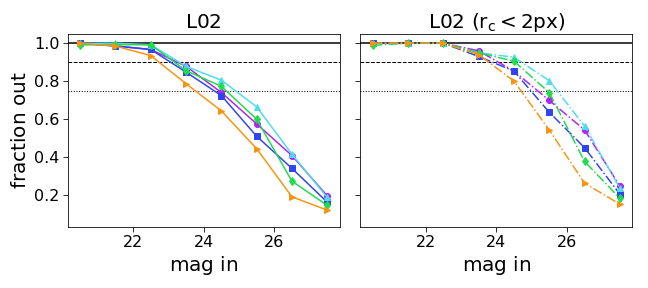


Appendix B Additional studies of the clump SFR
B.1 Clump SFR from de-reddened UV luminosity
in Section 4.3 we analysed the SFR of clumps derived from luminosities, with the simplifying assuming that clumps have no extinction. In this appendix we repeat the analyses of Section 4.3, de-reddening the luminosity of each clump by its internal extinction, using the values derived in Messa et al, (in prep). The luminosity is then converted into a SFR using the same Kennicutt & Evans 2012 relation used in Section 4.3. The distribution of the E(B-V) values for all LARS clumps is shown in panel a of Fig. 18. The distribution is peaked on zero extinction.
Panel b of Fig. 18 show the updated clumps’ SFR-size relation, with the de-reddened SFR values. The median SFR density of clumps increases times, going from to for the total sample and from to for the sub-sample, as can be appreciated in the figure. Therefore, even if the majority of clumps are weakly extincted, the effect on the clumps’ is significant.
B.2 Fit of the clumps relation
We fitted the clumps relation using the functional form . As described in the text we assumed the Kennicutt & Evans 2012 relation for the conversion between SFR and luminosity. We assume for this fit no internal extinction for the clumps and we use a simple least-squares fitting method. We compute the fit both considering the total sample and the HF sub-sample. In both cases, the sample of clumps is divided in two according to their using as separating value. Results of the fit are given in Fig. 19. We do not find a considerable difference between the different sub-samples.
B.3 Median SFR of clumps in sub-samples
We divided the LARS galaxies in sub-samples in function of their properties and in particular focusing on their SFR surface density, and stellar mass. For each property we dived the sample in two, using as separating values =, and . The median clump of each sub-sample is reported in Tab. 11.
| Sample | Included | median() | median(,HF) |
|---|---|---|---|
| () | () | ||
| (1) | (2) | (3) | (4) |
| 2,3,4,6,8,9 | |||
| 1,5,7 | |||
| low | 2,5,7 | ||
| high | 1,3,4,6,8,9 | ||
| low | 1,2,5,6,7 | ||
| high | 3,4,8,9 |