Distinguishing cosmologies using the turn-around radius near galaxy clusters
Abstract
Outside galaxy clusters the competition between the inwards gravitational attraction and the outwards expansion of the Universe leads to a special radius of velocity cancellation, which is called the turn-around radius. Measurements of the turn-around radius hold promises of constraining cosmological parameters, and possibly even properties of gravity. Such a measurement is, however, complicated by the fact that the surroundings of galaxy clusters are not spherical, but instead are a complicated collection of filaments, sheets and voids. In this paper we use the results of numerically simulated universes to quantify realistic error-bars of the measurement of the turn-around radius. We find that for a CDM cosmology these error-bars are typically of the order of . We numerically simulate three different implementations of dark energy models and of a scalar dark sector interaction to address whether the turn-around radius can be used to constrain non-trivial cosmologies, and we find that only rather extreme models can be distinguished from a CDM universe due to the large error-bars arising from the non-trivial cluster environments.
1 Introduction
The turn-around radius is the unique distance where the gravitational pull of large cosmological structures exactly cancels the expansion of the Universe. It therefore provides a special place to constrain the properties of the expanding universe, for instance the amount of dark energy [1, 2], or the force of gravity from the gravitational structures [3, 4]. The main observational difficulty with a measurement of the turn-around radius is that the 3-dimensional position of galaxies is very difficult to obtain, since only the 2-dimensional position on the sky is readily observable. For very nearby objects it may be possible to measure the turn-around radius directly [5]. This complication at cosmological distances may be overcome if one could measure a coherent motion of some of the galaxies. One such possibility was suggested in [6], where it was demonstrated that galaxies in large 2-dimensional sheets in their early phase of gravitational collapse indeed have properties allowing one to determine the full 3-dimensional spatial distribution. From numerical simulations it is known that these large structures are Zeldovich pancakes (also called sheets), which are over-densities that have only collapsed along the one dimension [8, 7]. In reference [9] it was proposed that it is possible to use a detection of such a sheet to actually measure the turn-around radius. This method has subsequently been investigated in a series of papers, in order to measure properties either of the clusters or of the expanding universe [10, 11, 12, 13, 14, 15, 16]. It was recently suggested that CDM model and an f(R) model of modified gravity could fairly easily be distinguished in the future, by measuring the turn-around radius and the virial mass [17] (see also [18, 19]). Most of the analyses mentioned above assume that the gravitational potential of the large cosmological structures are approximately spherical, and that the measured turn-around radius in a given direction therefore provides a fair representation of the turn-around radius of the galaxy cluster. The departure from sphericity around a galaxy cluster does, however, induce a large scatter in the measured turn-around radius. This is because the coherently moving galaxies (Zeldovich pancakes) which are used to measure the turn-around radius, are quite localized in space, and hence highly directional. In this paper we will first of all check to which degree this is an accurate approach, and at the same time we will quantify the magnitude of the error-bar of the measured turn-around radius. It turns out that the corresponding error-bars are significant, and must be included in future analyses. We then use this result to evaluate to which degree one can actually use measurements of turn-around radii to constrain alternative cosmologies. As concrete examples we consider the numerical implementations of three dark energy models and of a scalar dark sector interaction, which can be compared with the standard CDM cosmology. We demonstrate that a correct inclusion of the systematic error-bars is very important, and makes it rather difficult to distinguish between different cosmologies.
2 Turn-around radius
Figure 1 exemplifies the non-triviality of uniquely defining the turn-around radius for realistic cosmological structures. The green dots show particles within 10 virial radii of the cluster. The larger, red triangles show particles which have the property that they have zero radial velocity with respect to the central cluster (plus/minus 100 km/sec), and should thus represent particles at the turn-around radius. The red particles shown in the left panel are selected from a thin slice of width half a virial radius, and we only select particles outside of two virial radii, since the particles inside the virial radius on average are all at rest with respect to the centre. The filled, central circle represents 1 virial radius. The red circle is a guide-the-eye line at 5 times the virial radii.


The problem is clearly seen on the left panel of figure 1, namely that it is very difficult to define a unique turn-around radius. First of all, in directions in space with significant substructure, the turn-around radius may appear significantly closer to the cluster, because the gravitational potential of the large substructures affects the flow.
The second issue is, that it is not easy to observationally select a spatial slice, because it is virtually impossible to measure the line-of-sight distance to a given galaxy. Therefore a more realistic representation would be the right panel in figure 1. This figure demonstrates the necessity of first identifying some coherence between some of the galaxies, for instance by first finding a sheet, as proposed in [6].
The large substructures on the r.h.s. of Figure 1 appear to have zero radial velocity. That is mainly an effect of the use of "large" symbols, and the fact that we here colour-code all particles with zero velocity plus/minus 100 km/sec. This velocity range was chosen to make the infall galaxies visible on the l.h.s. of Figure. 1. The substructures each have a significant internal velocity dispersion, and only a fraction of their particles happen to have zero radial velocity with respect to the direction towards the nearby galaxy cluster at this specific moment in time.
Some of the zero-radial-velocity particles may happen to be splashback particles (returning towards the cluster after a recent merger). Such particles are not likely to end up as coherently moving galaxies (like in a Zeldovich pancake) so we have not studied this further.
3 Finding the turn-around radius
Measuring the turn-around radius requires a few steps [9]. The first is to find a collection of galaxies whose motion is somehow correlated. The simplest choice is probably to select galaxies which form part of a Zeldovich pancake [6]. These are identified as lines in observational phase-space, which is the directly observationally space spanned by projected radial distance and line-of-sight velocity. Some of the disadvantages of using the Zeldovich pancakes are that they are almost invisible on the sky (their projected spatial over-density is quite low), and secondly that they must be viewed at an angle between 20 and 70 degrees with respect to the line-of-sight [7]. The advantage is, that once found, the infall velocities of the galaxies belonging to the pancake is coherent. This allows one to determine the viewing angle of the pancakes, and thereby the actual radial distance to the nearby galaxy cluster can be determined [6].
The next step is to use that the radial velocities of galaxies near a galaxy cluster are the sum of two terms, namely the expansion rate of the Universe, , and the peculiar velocity, , which is negative due to the attractive force of gravity directed towards the large nearby galaxy cluster. One thus has
| (3.1) |
It happens that the peculiar velocity typically follows the simple form
| (3.2) |
where the coefficient is of the order for massive galaxy clusters [6]. This shape of the peculiar velocity profile is often valid in the range between 3 and 10 virial radii. The virial radius, , is here defined as , namely the radius within which the average density is 200 times the average density of the universe. The constant is a normalization to be determined. The detailed coefficients of equation (3.2) are, however, both dependent on the cluster mass and redshift [6, 13]. In the analysis of this paper we will only use the fact that the shape is given by equation (3.2), and we will even allow the coefficients to be different for different directions around a given galaxy cluster.
The last step is now to solve eq. (3.1) for , which directly gives us the turn-around radius [9]. In a future actual measurement one would also have to propagate the error-bars on the Hubble parameter and on the measured galaxy positions. For the present analysis we do not need to consider these.
In this paper we wish to measure the general scatter in the turn-around radius near galaxy clusters, and we therefore use all 49 directions in space. This means that in this paper we do not need to identify Zeldovich pancakes. Instead, we take the full region near galaxy clusters directly from a numerical simulation, and solve eqs. (3.1) and (3.2) to find in 49 directions in space.
4 Spatial cones
For each numerically simulated galaxy cluster we wish to investigate the effect of non-sphericity on the determined turn-around radius. In order to quantify the variations along different directions in space, we separate the sphere into cones of equal size. This fraction is chosen to resemble the fraction on the sky covered by a Zeldovich pancake [6, 7]. The peculiar velocity of the particles in each cone are now averaged in spherical bins, and the result is shown in figure 2. The solid, red curve is the spherical average of the full sphere. This figure shows a particularly well-behaved and relaxed cluster, and therefore the infall profiles are similar in all directions. In the innermost region (inside 1 or 2 virial radii) we see that the peculiar velocity equals minus the Hubble expansion, in such a way that the average radial velocity is zero in eq. (3.1). At large radii (from about 4 to 10 virial radii) the peculiar velocity is seen to slowly go to zero. The spherical average is seen to represent a fair average of the 49 cones.
A much more typical infall velocity picture is shown in figure 3. First of all we see a larger spread amongst the velocity profiles of the 49 directions, and a few of the directions are even seen to have positive peculiar velocities (crossing zero around 8 virial radii for this specific cluster). A few of these directions are here color-coded red. The cause of these positive peculiar velocities are large nearby structures, whose potentials significantly perturb the velocities of the particles in those directions. This is clearly seen in figure 4, where those regions are again color-coded red (triangles, at 4 o’clock). Another problematic peculiar velocity curve is seen in figure 3 to depart from the average trend around 6 virial radii, and becoming larger (more negative) at increasing radii. A few of these directions are color-coded blue. This is another feature of large, nearby substructures, as clearly seen on figure 4 (squares, at 1 o’clock).

When we identify Zeldovich pancakes on the sky, it is straightforward to avoid directions in space which have large overdensities of galaxies. We therefore assume that these directions have been identified, and we will remove them from the following analysis. Concretely, for this paper we use a simplified approach, and perform the following two tests. First, if the velocity profile along a specific direction happens to have positive peculiar velocity, then we remove that direction from the analysis (corresponding to the red lines in figure 3). Secondly, for any given direction in space, we will fit a power-law to the peculiar velocity both between 3-5 and 5-7 virial radii, and if any of the power-law coefficients are negative, then we remove that direction (corresponding to the blue lines in figure 3).
All the remaining directions will have slightly different infall profiles, and in order to measure a realistic error-bar for the determined turn-around radius, we will compare the variation amongst all these directions.
For each direction we now fit a power-law to the peculiar velocity in the radial range virial radii
| (4.1) |
Including slightly smaller/larger radii has very small effect on our conclusions. Since we know the full radial velocity is given by
| (4.2) |
we can find the turn-around radius by solving for the radius [9]. For each cluster we now have up to 49 values for the turn-around radius. As a measure of central value and error-bars we use the , and percentiles. Since the distribution of the turn-around radii is unknown, we also compare with error-bars estimated by fitting a Gauss (as well as an inverse-gamma distribution) to the distributions of turn-around radii, and we find no statistically significant change in any conclusions.

We select 100 massive clusters in the mass-range in a given numerical cosmological simulation. Considering first a standard CDM cosmological simulation, we plot the central turn-around radius with error-bars as a function of virial mass in figure 5. From this figure we see two things, first of all that the error-bars are rather significant for any given cluster, typically of the order . For equilibrated and fairly isolated clusters this may be as low as , and for less equilibrated clusters as high as . And second, that there are large variations from cluster to cluster, even for similar mass clusters. The relative error-bars are shown in figure 6 for 100 clusters from a CDM simulation.
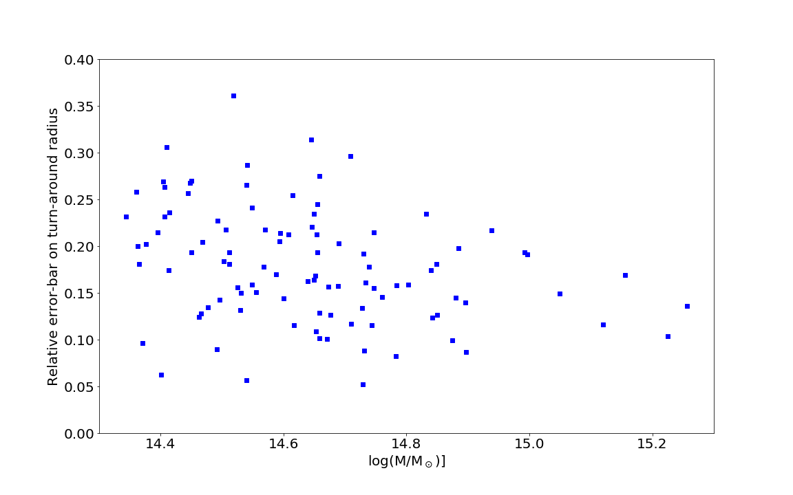
The trend of the mass-dependence of the turn-around radius can be approximated with a line of the shape
| (4.3) |
Today less than 10 Zeldovich pancakes have been identified, and yet we are considering using 100 as a future goal. In principle one could generalize the statistical analysis in the present paper by varying the number of clusters. We leave that for a future analysis.
5 Various cosmologies
In order to quantify the capability of the turn-around radius to constrain non-standard cosmologies, we shall consider three different classes of scalar field theories embedded in the action
| (5.1) |
where is a free function of the scalar field and . and describe couplings of the cold dark matter and baryonic matter fields, and , to the metric field defining the Ricci scalar . Furthermore, with bare gravitational coupling .
In the following, we shall briefly introduce the three specific models of interest: quintessence (Sec. 5.1) and -essence (Sec. 5.2) dark energy and a scalar field interaction between cold dark matter particles (Sec. 5.3). In Sec. 6, we will then describe the numerical implementations and simulations.
5.1 Quintessence
Quintessence [32, 33] theories are the archetypal dark energy models and are described by Eq. (5.1) with the choice of with a canonical kinetic contribution, linear in , and the scalar field potential . The models are minimally coupled to the matter sector with . The freedom in choosing can be represented by the freedom in choosing the time dependent dark energy equation of state , where
| (5.2) |
and dots indicate derivatives with respect to cosmological time .
5.2 k-essence
The -essence [34] models describe a class of more exotic dark energy models with noncanonical kinetic contributions in , nonlinear in , that are minimally coupled to the matter fields (). The freedom in the choice of function introduces an additional freedom over the quintessence models with the squared nonluminal sound speed of scalar field fluctuations
| (5.3) |
in addition to
| (5.4) |
where subscripts of denote derivatives with respect to .
5.3 Scalar dark sector interactions
As a third example, we study the interaction of cold dark matter with the scalar field , specified by the choices , a minimal coupling to baryons , and nonminimally coupled dark matter particles . We choose an interaction
| (5.5) |
and a potential of the form
| (5.6) |
with
| (5.7) |
where is the Ricci scalar evaluated at the current cosmological background and is the model parameter with . For the background matches that of CDM, and for our analysis we shall adopt the parameter value .
Note that we have chosen the model such that the dark sector interaction reduces to the Hu-Sawicki () gravity model [22] in the absence of baryons (). In this case, . The correspondence follows from applying the conformal transformation of the metric in the limit of (). The resulting coupling to the Ricci scalar can be cast as such that the Lagrangian density of the gravitational sector becomes with . For simplicity, we will assume here that all matter is in the form of cold dark matter such that the models become equivalent. Stringent Solar-System constraints on gravity, relying on a baryonic coupling, however, no longer apply. Cosmological constraints [23] such as from the abundance of clusters that are largely independent of the baryonic coupling require [24, 25, 26].
The choice of interaction (5.5) and potential (5.6) induces a chameleon screening mechanism for deep gravitational potentials . The potential wells for the structures considered in this work are, however, significantly weaker (). Screening effects can therefore be neglected, and we can adopt a linearisation of the interaction. More specifically, we linearise the quasistatic scalar field equation around the cosmological background such that [27, 28]
| (5.8) |
where the scalar field mass of the Yukawa interaction is given by
| (5.9) |
For the Poisson equation
| (5.10) |
this implies an enhanced effective gravitational coupling for the cold dark matter particles constituting , which in Fourier space is given by
| (5.11) |
6 Numerical simulations
To investigate the power of using the turn-around radius in distinguishing different cosmologies, we run simulations for -essence dark energy (Sec. 5.2) models and a scalar field interaction in the dark sector that reduces to linearised gravity in the absence of baryons. These can then be compared with a standard CDM simulation. The initial conditions for the simulations are set using the linear transfer functions from the linear Boltzmann code CLASS [21] at high redshift (z=100). All simulations use the same seeds as initial conditions. Our CDM simulations are performed using the gevolution code, which is a relativistic particle-mesh N-body code with a fixed resolution [20]. For the -essence and quintessence simulations we have used the -evolution code, which is a relativistic N-body code based on gevolution, in which the -essence scalar field and Einstein’s equations are solved to update the particles’ positions and momenta. Detailed tests of this code will be presented in [31, 30].
The simulation of the scalar dark sector interaction is performed through an implementation of the modified Poisson equation (5.11) in a Newtonian -body code based on gevolution [29], which has been validated against the results of Ref. [27].
We have thus four different simulations (in addition to CDM) to quantify the effects of a different background, clustering of a -essence scalar field and the effect on the clustering coming from the scalar dark sector interactions on the turn-around radius. All simulations have a comoving boxsize of Mpc/h, and discretize the fields on a grid of linear size N=512, giving a length resolution of Mpc/h. The dark matter phase space is sampled by N particles, corresponding to a mass resolution of /h. The detailed parameters of each simulation are shown in table 1.
| CDM | SDSI | quintessence | quintessence | -essence | |
| [] | 0.05 | 0.05 | 0.05 | 0.05 | 0.05 |
| 0.022032 | 0.022032 | 0.022032 | 0.022032 | 0.022032 | |
| 0.12038 | 0.12038 | 0.12038 | 0.12038 | 0.12038 | |
| 2.7255 | 2.7255 | 2.7255 | 2.7255 | 2.7255 | |
| 3.046 | 3.046 | 3.046 | 3.046 | 3.046 | |
| – | – | 1 | 1 | ||
| 0.687862 | 0.687862 | – | – | – | |
| – | – | 0.687862 | 0.687862 | 0.687862 | |
| – | – | -0.9 | -0.8 | -0.9 | |
| – | – | – | – | ||
| Initial redshift | 100 | 100 | 100 | 100 | 100 |
6.1 Results


We compare two of the non-trivial cosmologies with a CDM simulation in figures 7 and 8. The first impression is that it will be very difficult to distinguish between different cosmologies, because of the large error-bars for each cluster, and the large cluster to cluster variation. To that end a careful statistical analysis is needed.
One might wonder if it would be advantageous to consider galaxy groups (or galaxies [2]) to perform this analysis. That is, however, still not possible, because the turn-around radius is still only measurable using the Zeldovich pancake method, which only works near galaxy clusters. The reason is, that the Zeldovich pancake method relies on the gravitational perturbation exerted by the cluster on the nearby galaxy flow.
In order to address the problem of cosmic variance, we ran 3 extra numerical simulations of standard CDM universes, with different random seeds for the initial conditions. By comparing the analysis of each of these universes against the prediction from our first simulation we can estimate the magnitude of variance between different representations of the same cosmology. To that end we fit the first CDM simulation result by a fit of the shape given in eq. (4.3), . This is then used in a chi-squared comparison where we use a sum over the clusters
| (6.1) |
Here we use symmetrized error-bars for (average of upper and lower error-bars). Our first simulation has per degree of freedom of , indicating that the error-bars are reasonable.
Comparing with each of the other CDM simulations leads to between 1 and 6. This implies that when any given cosmology is contrasted with the CDM, then any less than approximately 6 will not allow us to distinguish the two.
When we perform the same statistical estimator for the simulations of quintessence or -essence (see the cosmological parameters in table 1) we get less than 6 for all the cosmologies. This implies that none of the cosmologies will be distinguishable from CDM.
The same statistical estimator for the simulations of SDSI cosmology gives , and thus indicates that it will (as the only one amongst the ones considered here) be distinguishable from CDM. Formally one might think that implies that for the two free parameters used in the fit, the two cosmologies are distinguishable at CL, however, that estimate does not include the cosmic variance, and the real CL is therefore smaller. A careful analysis of the statistics would require a larger number of simulations and is beyond the scope of this paper.
The entire analysis presented above has been based on observations at redshift zero. It is clear that different cosmologies have different evolution and structure formation, and it is therefore likely that an analysis including the redshift dependence will lead to somewhat stronger constraints than what we have obtained here.
7 Conclusions
The environments of galaxy clusters are complex distributions of sub-structures, filaments, sheets and voids. This implies that the turn-around radius, where the radial velocity of galaxies is zero, varies when different directions in space are considered. This implies that one must include a systematic error-bar when measuring the turn-around radius in the future. We use CDM numerical simulations to quantify the magnitude of this error-bar, and we find that it is about of the measured turn-around radius for typical clusters, going down to about for the most equilibrated and spherical structures. Furthermore, we show that one must carefully avoid measuring the turn-around radius along directions with large sub-structures.
We use a range of non-trivial cosmological simulations to gauge to which extent the inclusion of this realistic error-bar allows one to measure a departure from a CDM universe, and we find that it becomes possible only for the most extreme cosmologies we considered, such as scalar dark sector interaction with fairly large interactions.
Acknowledgments
It is a pleasure to thank Mona Jalilvand and Julian Adamek for support with the numerical simulations. SHH is grateful to the Swiss National Science Foundation and Carlsberg Foundation for supporting his visit to University of Geneva. This project is partially funded by the Danish council for independent research, DFF 6108-00470. L.L. acknowledges support by a Swiss National Science Foundation Professorship grant (No. 170547). FH and MK acknowledge funding by the Swiss National Science Foundation. This work was supported by a grant from the Swiss National Supercomputing Centre (CSCS) under project ID s710.
References
- Pavlidou et al. [2014] Pavlidou, V., Tetradis, N., & Tomaras, T. N. JCAP, 5 (2014) 017
- Pavlidou & Tomaras [2014] Pavlidou, V., & Tomaras, T. N. , JCAP, 9 (2014) 020
- Faraoni [2016] Faraoni, V. Physics of the Dark Universe, 11 (2016) 11
- Cataneo & Rapetti [2018] Cataneo, M., & Rapetti, D. International Journal of Modern Physics D, 27 (2018) 1848006-936
- Hoffman et al. [2018] Hoffman, Y., Carlesi, E., Pomarède, D., et al. 2018, Nature Astronomy, 2, 680
- Falco et al. [2014] Falco, M., Hansen, S. H., Wojtak, R., et al. MNRAS, 442 (2014) 1887
- Brinckmann et al. [2016] Brinckmann, T., Lindholmer, M., Hansen, S., & Falco, M. JCAP, 4 (2016) 007
- Wadekar & Hansen [2015] Wadekar, D., & Hansen, S. H. MNRAS, 447 (2015) 1333
- Lee et al. [2015] Lee, J., Kim, S., & Rey, S.-C. ApJ, 815 (2015) 43
- Lee et al. [2015] Lee, J., Kim, S., & Rey, S.-C. ApJ, 807 (2015) 122
- Lee & Yepes [2016] Lee, J., & Yepes, G. ApJ, 832 (2016) 185
- Lee [2018] Lee, J. ApJ, 856 (2018) 57
- Lee [2016] Lee, J. ApJ, 832 (2016) 123
- Lee [2017] Lee, J. ApJ, 839 (2017) 29
- Lee & Li [2017] Lee, J., & Li, B. , ApJ, 842 (2017) 2
- Rong et al. [2016] Rong, Y., Liu, Y., & Zhang, S.-N. MNRAS , 455 (2016) 2267
- Lopes et al [2019] Lopes, R. C. C., Voivodic, R., Abramo, L. R. & Sodré, L., JCAP 1907 (2019) 026
- Lopes et al. [2018] Lopes, R. C. C. Voivodic, R., Abramo, L. R. & Sodré, L., JCAP 1809 (2018) 010
- Capozziello et al. [2018] Capozziello, S., Dialektopoulos, K. F. & Luongo, O, Int. J. Mod. Phys. D 28 (2018) no.03, 1950058
- Adamek et al. [2016] Adamek, J., Daverio, D., Durrer, R., & Kunz, M. , JCAP, 7 (2016) 053
- Blas et al. [2011] Blas, D., Lesgourgues, J., & Tram, T. , JCAP, 7 (2011) 034
- [22] Hu & Sawicki, Phys. Rev. D76 (2007) 064004.
- [23] Lombriser, Annalen Phys. 526 (2015) 259.
- [24] Schmidt, Vikhlinin & Hu, Phys. Rev. D80 (2009) 083505.
- [25] Lombriser, Slosar, Seljak & Hu, Phys. Rev. D85 (2012) 124038.
- [26] Cataneo, Rapetti, Lombriser & Li, JCAP 12 (2016) 024.
- [27] Schmidt, Lima & Oyaizu, Phys. Rev. D79 (2009) 083518.
- [28] Lombriser, Koyama, Zhao & Li, Phys. Rev. D85 (2012) 124054.
- [29] Hassani, F., Lombriser, L. 2020. arXiv:2003.05927.
- Hassani et al. [2020] Hassani, F., L’Huillier, B., Shafieloo, A., Kunz, M., Adamek, J. , JCAP 04 (2020) 039.
- Hassani et al. [2019] Hassani, F., Adamek, J., Kunz, M., Vernizzi, F. , JCAP 12 (2019) 011.
- [32] Wetterich, Nucl. Phys. B302 (1988) 668.
- [33] Ratra & Peebles, Phys. Rev. D37 (1988) 3406.
- [34] Armendariz-Picon, Damour & Mukhanov, Phys. Lett. B458 (1999) 2019.