Intertemporal Community Detection in Human Mobility Networks
Abstract
We introduce a community detection method that finds clusters in network time-series by introducing an algorithm that finds significantly interconnected nodes across time. These connections are either increasing, decreasing, or constant over time. Significance of nodal connectivity within a set is judged using the Weighted Configuration Null Model at each time-point, then a novel significance-testing scheme is used to assess connectivity at all time points and the direction of its time-trend. We apply this method to bikeshare networks in New York City and Chicago and taxicab pickups and dropoffs in New York to find and illustrate patterns in human mobility in urban zones. Results show stark geographical patterns in clusters that are growing and declining in relative usage across time and potentially elucidate latent economic or demographic trends.
1 Introduction
Much research has been done in recent years in the analysis of real world networks. One particular area of active interest is community detection. Broadly, community detection is an unsupervised exploratory data analysis method that extracts subsets of vertices in a network that are more densely connected within the subset than between the subsets in a given network.
A majority of the research on community detection in networks has dealt with static networks [1]. However, many real-world networks exhibit dynamic properties, such as human mobility networks in urban systems. These networks include commuting patterns over time [2], location based social networks [3], taxicab travel patterns [4] and cell phone call records [5]. Understanding the structures of these networks reveals underlying trends in human mobility and provides important information for the management of urban infrastructure.
There are many human mobility patterns that can be represented as networks with high temporal resolution because of the presence of origin and destination locations and time stamps associated with the trips. For example, bikeshare systems are rich and remarkably comprehensive in tracking mobility patterns within a city. By 2019, over 2,000 cities have created bikeshare systems around the world. In 2018, according to the National Association of City Transportation Officials, 36.5 million trips were completed in over 100 cities in the United States using these systems. Many of these systems have stations where users can rent the bikes and deposit them at another station at the end of the trip. These stations allow the system operator to track the precise origins and destinations of individual trips by time-of-day and day-of- week. Another mode of travel in cities is by automobile, which trips can be modeled as networks. In particular, taxicabs in cities are regulated and therefore location and time data of these cab pickup and dropoff locations are often reported to the regulators. The increased usage of often less-regulated ridesharing services (Uber, Lyft etc.) have reduced taxi trips in the last few years. Much research has been done on network analyses [6, 7] [8, 9], but most do not fully take into account the dependencies induced by the network structures and temporal trends. Many of these studies have also focused mostly on demand estimation [10, 11].
In this work, we develop a method to identify clusters of significantly connected nodes in a time-series of weighted networks. Identification of such clusters allows us to understand the nature of geographical, economic and cultural relationships, when these networks are rooted in cities. Identifying trajectories of connectivity in clusters across time may reveal structural changes within the mobility patterns in the city. We develop an intertemporal community detection method to analyze the structure of long-term trends in time-series of networks to understand global and local trends. In particular, we attempt to determine whether such trends are uniformly distributed across the networks, or whether certain communities exhibit countervailing trends in interconnectivity when compared with others. We aim to identify and partition the nodes that potentially have driven this global trend, as well as the communities that exhibit locally specific trends.
The objective of the community detection method in this study is to find groups of nodes that are consistently connected across time and exhibit increasing, decreasing, or stable trends in connectivity. We use the assumptions of the weighted configuration model as posited in [12, 13] to scale and whiten the time-series of node-set connectivities. In doing so, we remove much of the overall graph effects that represent network-wide signals at a given time-point, such as weather and other city-wide phenomena. Though normalization removes much of the seasonality, some autoregressivity still persists: we ignore these effects but future work should account for such behavior. Analysis of time-varying weighted graphs allows us to gain more insight into the nature of the city as a complex accumulation of micro-level spatial activity patterns. While this method of intertemporal community detection is developed for data structured like mobility systems, it can be adapted for any type of time-series network data with registered nodes (such as inter county commuting patterns, internet traffic, etc.)
2 Data and Network Construction
We apply intertemporal community detection to data from two bikeshare systems and a taxicab trips. Bikeshare trip data for Divvy (Chicago) and Citibike (New York) are publicly available on their respective websites [14], [15]. The two bikeshare systems provide contrasting cases. Divvy ridership increased steadily between 2014-2016 from 2.7 to 3.6 million, but overall ridership declined slightly from 3.8 million trips in 2017 to 3.6 million in 2018 [16]. The Citibike system, on the other hand, has consistently increased in usage from 14 million in 2016 to 16 million in 2017 and 18 million in 2018 [15].
The publicly available datasets include trip start and stop times for each trip between stations. In our analyses, we focus on the time period between July 2016 and June 2018. We omit all stations that were newly introduced or removed within this period. 547 nodes (7.4 million trips) in Chicago and 583 nodes (8.4 million trips) in New York remain in the dataset used for this study. One common problem in bikeshare systems is the issue of supply-demand mismatch in ridership. A station in a high-activity area of a large city is often empty or full at certain times of the day [17, 18, 19, 20, 21, 10]. A full or empty station prevents an otherwise possible trip. Load rebalancing is a well-studied problem for bikeshare systems in order to solve the inefficiencies associated with queuing between bikes in stations with finite numbers of slots for bikes at each station. Real-time data on station status rebalancing exist for New York and Chicago [22]. However, historical station inventory data is only available for New York City [23] and not Chicago. Thus, for the New York bikeshare system, we find communities with and without demand adjustment (see section A.1 for details on the method).
The taxicab data for New York is from the Taxicab and Limosuine Commission [24]. We use data from January 2017 to 2019 because trips from the ridehailing apps (such as Uber, Jio) are only included since 2017 in the data. 263 zones cover all the five boroughs of New York, and the dataset includes over 453 million trips between these zones.
From these datasets, we construct the observed time-series of networks as . In all these datasets, we aggregate the trips between a pair of nodes for each week. The weekly aggregation smooths the diurnal variations and keeps the time-series long enough for time-domain. Thus, each time corresponds to a week, where is the total number of time periods. The indicator represents the presence of any trips at time between and . We use the number of trips between two nodes per week as the edge weight . In network the degree of node is defined as and strengths are defined as at each time-unit across total time [13]. We define the index set as the set of all nodes , which represent stations.
3 Detecting Intertemporal Communities
In this section, we describe a method based on iterative testing of node-set connectivities to extract statistically significant communities across time [13, 12]. We use a similar approach but account for and classify the types of time dependency. We posit that trends across time are generally increasing, decreasing or stable and account for these types of time dependence. To this end, we adjust connectivities to time-decay and find trends using equivalence testing [25, 26].
We introduce a method to find clusters that are significantly connected across time and exhibit differing trends in connectivity by building on the iterative testing framework of Palowitch et al.([12]). In that work, the weights on the edges incident on each node are modeled as
| (1) |
where each represents the degree of node , where each represents the strength from node , and represents the global sum of strengths and degrees.
Communities are sets of vertices that have edges that are significantly interconnected within the set but not connected outside the set. Prior work [12, 13] use the above null model to identify communities within a single graph. Random variables with variance are constructed so as to satisfy the weighted configuration model [13, 12]. When are structured in time-series, the variances of random variable summarize the overall variability of each network across time. We utilize these time-varying characteristics of the networks to find intertemporal communities.
3.1 Intertemporal Configuration Null Model
We extend the method used in prior work [12, 13] by developing an intertemporal null model wherein a baseline model is extracted from a time-series of registered networks and iteratively subjected to hypothesis tests for trends and local deviance. We detect significant communities across the time-series of networks if the trend and variation components are significantly different from those of the baseline model. These communities signal subsections of the network that are either strongly interconnected at either the beginning or end of the time-period, or consistently connected throughout the entire time period.
We define the intertemporal null model for a given node set (as in [12, 13]) to determine if it is significantly interconnected across all time-points according to the hypothesized trend. We search for communities that are
- •
increasing if its nodes are significantly connected at time , but not necessarily significantly connected as is late.
- •
decreasing if its nodes are significantly connected at time , but not necessarily significantly connected when is early.
- •
stable (or neutral) if its nodes are significantly connected across all time points.
Within , we posit that a time-series of relative connectivity may be decomposed into trend and variation components. Trend denotes the presence of a constant time-trend in the relative connectivity amongst nodes in set . Variation denotes the aspects of the node-set connectivity that do not vary systematically across time.
3.1.1 Null Model for Node-Set Connectivity
The estimate for each edge weight at time is a simple extension of (1), which is the null model for a single graph.
| (2) |
Each is an weighted edge on a random time-varying graph , where each has fixed degrees and strengths . Each graph at time has total degrees and total strengths . The analogous node-set connectivity (as [12]), is
| (3) |
with means and variances
| (4) | ||||
| (5) |
detailed derivations of these values can be found in the text of [12].
To search for intertemporal clusters, we investigate the significance of connectivities of to across time . The normalized connectivity score represents the sums of weights of a given node set in graphs :
| (6) |
3.2 Identifying Nodes that are Significantly Bordering Across Time
We use iterative testing to identify nodes that are significantly connected to their neighbors through time. Methods developed in previous literature [12, 13] have applied this method to a fixed graph . We use the same method of deriving significance of the probability that is significantly connected to in set as in Palowitch et al. ([12]).
The proposed algorithm relies on an iterative procedure starting at iteration step , then repeated until the results do not change. The objective is to find sets such that for each , is significantly connected to across all time points . At a given step , for fixed time , for a set of nodes and a bordering node , the score of node-set connectivity is determined by (3):
| (7) |
After the normalizing calculation (6) is performed, a p-value for each is then determined:
| (8) |
For each time point , the p-value is then corrected for false-discovery rate correction as in [27]. The non-significant nodes are rejected and the a set of significant nodes is retained. We describe additional steps to find significant nodes in the following sections 3.2.1 - 3.2.2 to account for time-decay in significant bordering nodes and describe the testing of trends in 3.3.
3.2.1 Time-Decay Adjusted False Discovery Rate Correction
To identify significantly interconnected nodes for a given time , a slightly augmented version of the Benjamini-Hochberg [28] procedure used in [12, 13] is used. The only difference is that the FDR-adjusted p-value is multiplied by decay term , contingent on if the communities are hypothesized to be increasing, decreasing, or stable in connectivity over time. For a fixed time , iteration step , and set , we find all the nodes that are significantly connected to across all time after calculating the p-value as in (8). The output set at iteration and time is written as , described in more detail in later sections in equation (11).
We define is an exponential decay term to adjust for the shifting time-window of significance. It is defined as:
| (9) |
The terms and are defined such that is 0 at time 1 and 1 at time if the trend is increasing, and 1 at time and 0 at time if the trend is decreasing:
If the trend is posited to be increasing, then the algorithm allows more permissive selection of ‘significantly’ bordering nodes when time is early, but is more penalizing when approaches . When is 1, then is equal to zero. In this case, all are zero and will automatically be counted as significant if borders . When is , then is 1, so the FDR correction is identical to BH. The threshold for the maximum allowable p-value increases as decreases so that negligible connections (when is early) that become stronger (when is late) are deemed significant.
Conversely, when the trend is posited to be decreasing, the same kind of correction is made in reverse because the multiplier is subtracted by one. Because the multiplier to the adjusted p-value is always less than 1, the procedure is always less conservative than the Benjamini-Hochberg method and lets nodes that otherwise would not be significant at a given time-period be deemed as“significant” based on their potential to be significant given their trajectory. If the trend is posited to be neutral, then we use the ordinary BH rejection procedure.
3.2.2 Bonferroni Interval for Bordering Frequencies
The previous section 3.2.1 details significance testing for the collections of nodes at each time period. To determine whether the collections of nodes are significantly connected to at all times, we apply a second testing step using Bonferroni Correction. This correction is applied to the frequencies of nodes whose p-values have been deemed significant by the BH correction (in the previous section). The product of Bonferroni confidence intervals is used to define the significance of the neighboring frequency at iteration step , for each across all time . For a set , we define as the set of nodes that are found to be ‘significantly bordering’ described by Section 3.2.1:
A large value of for all signifies a large collection of nodes that significantly border and results in a false discovery interval that is close to , and hence must border for nearly all time for it to be significant. Conversely, if is small, then the required frequency for to be significant is not as high. During this step, we assume away dependency between .
We define to be the threshold for false discovery interval of all significantly adjacent nodes to node
where is the Bonferroni confidence level at each time point. The product of these intervals cross all time multiplied by the total time gives the threshold of significantly bordering nodes across all time.
Now we define the as the combined list of all the nodes in any : For each , we define the bordering frequency as the counts of which are significantly bordering across all time . A significant suggests that is more frequently bordered across time than other nodes. Each significantly borders all if
| (10) |
that is, if borders enough times across for it to be significant overall in the time-period [29]. Finally, we take the union of all nodes that satisfy the “significantly neighboring” criteria (10) and denote the set
| (11) |
The resulting set represents the nodes that are significantly connected across time, given the appropriate time-window adjustments. We then check if the trends are actually as hypothesized.
3.3 Significance Testing for Trends
We define the sum of in (6) as to gauge the significance of the time-trend of a cluster.
| (12) |
Moreover, for a given community that is significantly connected across time , we write the vector of node-set connectivity as the sum of trend and variation components, where represents the trend component which is linearly dependent on time and represents the variation component that is stationary across time.
The previous sections describe discovery of node-sets that are significantly connected across time, this section details testing for their trends. If the trends are posited to be positive or negative, then one-sided t-tests are used, respectively with null hypotheses and . More detail can be found in the appendix (section A). If the the trend is positied to be negligible (stable), then the two sided test:
is used. The hypothesis is flipped (compared to the positive or negative tests) in order to test if the trend is equal to zero. We invoke equivalence testing methods ([26]) to determine significance in relation to a pre-selected symmetric interval about zero.
Given an set at iteration , we first find all nodes that are significantly bordering across time as described in Section 3.2 and label these nodes as as in (11). We then assess the significance of the trends of each of the nodes in relation to set . Calculation of trend employs test statistic for node-set connectivity :
| (13) |
Using and , we then find the time trend for each . We assume that intertemporal communities have trends that are increasing, decreasing, or neutral. We use the equivalence testing method to assess trend significance [25, 26] . Even if a trend is significant, its impact may be negligible and should be assumed to be “zero”. A bounding energy barrier is chosen to control the size of the desired time-trends. A positive is chosen as a lower bound for a positive trend, is used as a upper bound for a negative trend. A symmetric bounding interval of about zero is used for a neutral trend.
Hypothesis tests are conducted for the time trend for set (at iteration ) and node . Significances of trend (assuming fixed at iteration ) are calculated using the difference of the estimates with the upper bounds (if positive) and lower bound (if negative). T-tests for these differences or are then performed to assess significance while excluding very small trends. To determine whether a node-set has a significantly negligible (neutral) trend, we utilize the approach outlined by Dixon et al. [26] and use two one-sided tests to determine if is significantly outside the interval .
3.4 Iteration and Overlap Filtering Steps
After the procedures for selecting nodes that are both significant in connectivity (Section 3.2) and trend depending on the posited direction of trajectory (Section 3.3), we derive p-values from the -statistic of the time-trend . The nodes whose trends are significant after incorporating the FDR correction with significance level , are retained.
We update the set with the inclusion of the new nodes that are both significantly connected to across all time and have a significant trend according to the trend hypothesis. The procedure is repeated until the set becomes stable such that for all candidate sets. In all the applications used in this study, this process takes 3 to 5 iterations.
After stable sets are found from the iteration steps, they are filtered by their Jaccard overlaps [12, 13]. We use an overlap threshold of 0.50 to remove clusters with over 50% overlap; more details on this procedure can be found in prior work [12]. After filtering by Jaccard overlaps, communities of size 3 or less are removed, as dyadic or triadic relationships between nodes may be too localized to be meaningful in a larger scale.
3.5 Effect of Normalizing Edges
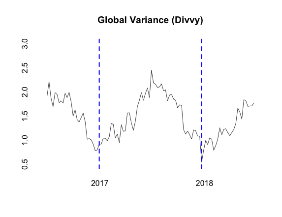
Modeling network time-series using the weighted configuration model places edge-weights in a relative scale when they are normalized by their expectations and variances, which are functions of global . Global is shown to be highly seasonal (fig. 2) in the Divvy system in Chicago but less so for the NYC taxicab and Citibike data. The variances in the taxicab data experience a sudden increase in the middle of 2017 and thereafter consistently increase through time. The high seasonality of in Chicago and the effects of its removal by normalization are apparent in figure 4. Scaling edge weights is especially useful in time-series networks where seasonal effects dominate much of the variation (in the Divvy data) or the trend (in NYC taxicab data).
Global Variance (Divvy; Citibike; NYC Taxicab)


4 Results
We report results for a range of values for tuning parameters and for observed demand .
In the Divvy Network, we fix at 0.05 and as well as because these settings capture clusters of moderate sizes across all trend categories and also show distinct geographical divisions. Under these tuning parameters, we find five clusters with decreasing connectivities over time and five clusters with increasing connectivities. We find only one cluster with a stable trend at the 0.05 significance level.
There is a stark division in trends between the northern and southern parts of the city (fig. 3). At the 5% significance level, clusters with significantly decreasing trends are mostly found in the southern and western parts of the city, while clusters with significantly increasing trends are mostly found in the northern and central parts of the city. Interestingly, the decreasing clusters map to a nearly concentric outer ring around the central part of the city, while the increasing clusters stretch from the Loop northwards along the shore of Lake Michigan. One stable cluster is located in the Loop.

It is useful to focus on one community to illustrate the effect of edge normalization (see section 3.2). In figure 4, while the raw edge weights show a stable trend, the normalization shows an increasing trend. Thus, the collection of five stations in the Lincoln Park neighborhood in Chicago is classified as a cluster with an increasing time trend rather than a stable one.
Sum of Edge Weights in Sample Community 

In New York City, many clusters are found in the Citibike system in networks of observed demand (raw counts of trips) (fig. 5). We set to 0.05 and to 0.007 and 0.009 to allow direct comparison to the clusters in the Divvy system in Chicago. When is set to 0.007, increasing and decreasing clusters are found throughout Manhattan and Brooklyn while stable clusters are mostly concentrated around Lower Manhattan. When is set to 0.009, increasing and decreasing clusters decrease in size and number but stable clusters increase in size and geographical scale: All of the land-area in Manhattan and part of north Brooklyn is covered in these stable clusters.

The geographical domain that the taxicab network covers is much larger than the bikeshare network, which only spans Manhattan and Brooklyn. In two settings of , clusters are decreasing in connectivity across much of the Bronx, Queens, and much of Brooklyn. Clusters are consistently increasing in eastern parts of Queens. One cluster appears to consistently link Staten Island to southern Brooklyn for both values of . Clusters are stable around the denser parts of the city, as is the case in Upper Manhattan when is 0.01 and in Upper and Lower Manhattan, Central Brooklyn, and Astoria in Queens when is 0.02.

4.1 Effect of Demand Correction
We apply the intertemporal community detection algorithm to the demand-corrected (DC) time-series networks with weights in the Citibike system. We use the same significance and set barrier to 0.007 and 0.009 as in observed trip networks in NYC and the Divvy system in Chicago. The obtained communities retain similar geographical characteristics as those in uncorrected graphs, but with some key differences.
When is set at 0.007, the decreasing and increasing clusters in the demand-corrected networks are localized in approximately similar geographical regions as in non-corrected networks. Increasing clusters are mostly located in Upper and Lower Manhattan as well as Southern Brooklyn. Decreasing clusters are present in some small areas throughout Manhattan but pervasively cover swathes of northern Brooklyn around the Williamsburg region. Stable clusters mostly span Midtown Manhattan but also extend to northern Manhattan and parts of Brooklyn.
When is increased to 0.009, the increasing and decreasing clusters shrink in size and number and the stable clusters expand. Increasing clusters are more visibly located in Upper and Lower Manhattan (similar to the clusters in the graphs of observed demand) at the higher threshold. Decreasing clusters are interspersed throughout the city but large coherent areas are more clearly located around northern Brooklyn, also as in the observed graphs . The stable graphs, however, are much larger and cover much more ground in Lower Manhattan (fig. 7) .

5 Discussion
In the Citibike, Divvy, and NYC taxicab systems, we observe a trade-off between increasing or decreasing clusters and stable clusters depending on the choice of . If is larger, then there is “more room” for a trend to be classified as stable, but less so for increasing or decreasing trends. Discovery of more increasing and decreasing clusters when is increased suggests that these clusters are increasing or decreasing in connectivity at different rates from the other clusters. When is large, increasing and decreasing clusters vanish but more stable clusters persist.
The interaction between and is not entirely linear or monotonic. Though a decrease in may correspond to an increase in , a lower implies that the nodes are more connected at each time-instance and does not necessarily mean that the trend is higher. Figures 5 and 7 show that in both and , clusters appear as becomes larger and stays the same. Such behavior may be attributed to FDR correction. A lower barrier may yield more significantly connected nodes but with weaker trends. The sensitivity of community detection to the choice of parameter is an important issue [6]. We compare the extracted communities under different tuning parameters and .
In results from the observed network in Chicago, the choices of and produce generally similar results over a range of values (fig. 3). Shifting from to induces discovery of more increasing and decreasing clusters, but the bound is too tight for any significant sets to be found under the hypothesis tests in (21).
More increasing clusters are found in high-traffic areas surrounding cultural amenities such as the Adler Planetarium in the Loop when . Several other clusters in the Near North Side and the Loop are found under this threshold that are not found under the settings in figure 3. Stable clusters are mostly found also in the Loop and the Near North Side and share a lot of commonalities with increasing clusters at less stringent thresholds; we deduce they have a moderate increasing trend.
Our analysis is exploratory in nature and only summarizes the trajectories of network structures in time but not their underlying causes. While this work is focused on methodological aspects of temporal community detection, results suggest that it might be useful to think about the causal mechanisms that underlie the different types of clusters in the bikeshare networks. The geographical patterns of the cluster map to different neighborhood characteristics.
Chicago is an conventionally viewed as a monocentric city focused on the downtown [10], so it is unsurprising that stable clusters are found around the Loop. The southwestern part of the city is comparatively less affluent. Pilsen, in particular, is a predominantly Latino neighborhood, although its demographic composition is rapidly changing due to gentrification [30, 31]. Lincoln Park and Lakeview are known to be affluent and mostly white residential neighborhoods. Increasing, stable, and decreasing trends map closely to these neighborhoods of differing socioeconomic characteristics and suggest latent factors undergirding the decreasing trends that are driving the overall slight decrease in trips from 2016 to 2018.
At the same fixed parameters for and , clusters in NYC are more numerous and less geographically spread out than Chicago, possibly because the city is much denser and more populous. Moreover, the seasons are milder, which induces less variation in trends. Figure 2 shows that the global variance parameter of the Divvy system is highly seasonal, unlike that of the Citibike system.
Several areas appear to be persistently decreasing in both demand-corrected and observed networks. The easternmost group of four stations in Williamsburg is found in both thresholds of in demand-corrected and observed networks, suggesting a plausibly real relative decreasing trend in this neighborhood.
Citibike has much higher overall usage and thus a lower significance level (compared to Divvy) is used to locate the clusters that are significantly anomalously connected. The Citibike system is globally consistently increasing as opposed to Divvy which is slightly decreasing from 2017 to 2018.
The edge-normalizing step of the community detection algorithm (section 3.5) makes such station-specific adjustments affect the whole network, thereby affecting the entire system. Regardless, similarities persist in clusters in both DC and uncorrected graphs. The demand corrected (DC) networks when is 0.007 and 0.009 yield similar decreasing clusters to those of the uncorrected networks .
Demand-adjustment makes a considerable difference in some clusters in the Citibike system. Among decreasing clusters, most of the discovered communities in both uncorrected and corrected graphs are located in Brooklyn, with some scattered around Manhattan (figs. 5, 7). However, clusters in general are smaller and less numerous in the DC case. The opposite case is observed for increasing clusters: discovered communities in DC graphs are much more geographically defined in Upper and Lower Manhattan and southern Brooklyn and notably much larger, more numerous, and overlapping. Stable clusters are confined to Manhattan in the observed graph , but appear to form different shapes and extend to Brooklyn in DC graphs .
Adjusting for demand-correction thus reveals stronger, more cohesive increasing trends within the ridership and suggests that observed trips do not adequately capture the latent increasing signals that are distorted by load imbalances from empty stations.
A common feature of decreasing clusters in both DC and non-DC networks across all choices of is the presence of large clusters around the Williamsburg neighborhood in north Brooklyn. Small pockets of the neighborhood are clustered into increasing or neutral clusters, but decreasing clusters are dominant. On the other hand, south Brooklyn has more of a mixture of trends. Though certain regions in DC and non-DC graphs are grouped into decreasing clusters, the decreasing clusters in DC graphs are very large, encompassing nearly all of the southern part of the city, with some clusters extending to southern Manhattan.
Due to the fact that trips by taxicabs are, in general, longer than the trips by bike, the clusters that are found cover larger areas. We choose to be 0.01 and 0.02 to maximize differentiation between clusters based on an assumed negligibility of trend. Most increasing clusters generally look the same with one exception. One of the decreasing clusters changes shape rather drastically as is increased from 0.01 to 0.02 and goes from covering nearly all of Brooklyn to covering northern Brooklyn and part of Queens. These patterns mostly demarcate general regions and may illustrate decline in usage within these areas due to other transit options such as bikeshares in Brooklyn and the Bronx. Increasing clusters are generally similar across choices of and highlight the corridor between Brooklyn and Staten Island, which may be illustrative of the lack of public transit between these regions. The neutral clusters only demarcate a small region around Central Manhattan when is 0.01, but expand to cover most of Manhattan when is 0.02. These patterns may be indicative of the consistent usage of taxicabs in the busiest parts of the city. There are some similarities between clusters of taxicab trips and Citibike trips: stable clusters are found around Central Manhattan in both cases (DC and non-DC cases for Citibike), and southern Brooklyn is found to be increasing (DC case) just as in the taxicab network (though the latter case is connected to Staten Island) However, because the geographical scale of the taxicab dataset is much larger than that of Citibike, and signal different kinds of mobility and connectivity, the similarities in clustering geographies may not be reflective of similar underlying trends.
Results in Chicago and New York illustrate the similarities and differences between the two systems. The Citibike system is larger than Divvy (18 million trips in 2018 vs 3.6 million) and is growing at a much faster rate. As such, the significance thresholds for connectivity are stronger for Citibike and its communities represent more densely connected collections of nodes. There are no large contiguous areas of consistent decreasing trends like in the ring of clusters surrounding Chicago’s city center (fig. 3). The decreasing clusters in Chicago may be indicative of specific geographical patterns that drive the global slight decrease in the Divvy system because the clusters are geographically coherent. However, the decreasing clusters in NYC are distinctively countervailing with respect to to the overall increasing global trend, though certain clusters (like in Williamsburg) are persistent across several settings and parameters.
Because the proposed method is for exploratory purposes, these summarizing claims should be verified in a more rigorous way in future research. Furthermore, the choice of varies by application. We use an ad-hoc scheme to select whose resultant neutral clusters yield approximately the same amount of nodes as the increasing and decreasing clusters combined.
However, because most of the results we present include two different values of in order to show the differences in results due to adjusting the parameters , the results in this study may not strictly adhere to this criteria. However, results from Fig. 3, Fig. 5 and 7 all approximately follow ths heuristic when , though they may have different ’s. Different applications of intertemporal community detection may call for different criteria for tuning parameters. For example, setting to be small so as to not allow discovery of any neutral clusters (i.e. Fig. 3, ) may also be a suitable option. In future work, more principled approaches for setting tuning parameters utilizing cross-validations may be investigated.
6 Future Work
In both Chicago and New York City, there may be several explanations for the underlying signals that cause the clusters to decrease in connectivity. Further work may examine what these signals are and how these signals may function. One explanation may be that decreasing trends are symptoms of displacement, destabilizing steady ridership among long-term inhabitants in gentrifying neighborhoods. Another may be differential rates of attention given to load rebalancing in stations in different neighborhoods with varying resources. Causal analysis of these phenomena are outside the scope of this study, but our exploratory results are useful in initializing conversations about changes in mobility patterns within and between neighborhoods. Future work may analyze the relationship between the discovered communities and factors such as new construction, bike lanes, weather, incomes, and demographic characteristics.
The methods devised in this study can be applied to a variety of data in network time-series format, particularly human mobility networks. The method can be applied to bikeshare networks in other cities, or may be applied to other networks of transportation in urban systems. Future work may elaborate on the theoretical properties of intertemporal community detection. The null model described in section 3.1 may also have further use in statistical inference or in forecasting future patterns. Another extension would be to account directly for the spatiotemporal aspects of trips in the methodology.
Our work currently relies on historic station inventory data for the analysis of the Citibike system. We do not have access to historical inventory data for Chicago and thus are not able to estimate demand. Though similarities between corrected and non-corrected networks in the NYC bikeshare system shows that there may be some use in using only non-corrected data in Chicago, there are limitations in drawing conclusions for demarcations of functional mobility zones using only observed demand. We propose a method in A.2, but further estimation of demand without historical station inventory data should be explored in future work in conjunction with community detection.
7 Conclusions
We proposed a novel method to cluster networks representing bikeshare systems that vary across time. Our community detection method combines usage of a configuration null model with a trend model to describe the expected trajectory of the graph evolutions. We use a significance-testing methodology to assess whether nodes are anomalously connected to each other within and across time-periods. By using the proposed method, we are able to filter some of the system-wide seasonal effects and map geographically coherent communities of latent human mobility signals in the bikeshare stations in Chicago and New York and the taxicab network in New York. The methods used in this paper may be applied to other situations where it is important to study the evolution of structures within networks.
Appendix A Appendix
A.1 Corrections for Forgone Trips Due to Load Imbalance Given Load Rebalancing Data
We estimate the functionals by taking the average rate at which a station is empty i.e. yields no available bikes. are calculated as the ratio of the time-intervals that a station is empty to the total intervals during peak-times (i.e. when users could plausibly check out or return bikes). The ratio represents the probability of a station being empty when a user accesses it. A high ratio signifies that the station is usually empty, and so it is more frequently load-imbalanced due to high usage, hence more weight should be proportionally accounted for to estimate the trips that could have been taken if the system was perfectly balanced.
Let be the event that a typical trip in year from or to station is foregone owing to load imbalance and let be its associated probability. is approximated as:
| (14) |
Observed demand for each edge between stations during time-index (weeks in this analysis) are then converted to estimated demand as follows:
We refer to the time-series of graphs comprised of these demand-corrected (DC) weights as . For this study, we assume that this probability is constant over the year. Seasonal effects may be influential in this calculation but will be deferred to future research. We assume that a full station induces a negligible impact on load imbalance compared to empty stations. Each probability is calculated as the proportion of time-intervals that the station is empty. We construct networks of estimated demand to correct for trips that could not have taken place due to full or empty stations and find communities within these networks to more accurately find communities of trip demand in a human mobility network [11, 32, 32].
A.2 Corrections for Forgone Trips Due to Load Imbalance Without Rebalancing Data
Though real-time data on station status (e.g. number of open slots) exist and are available online [22], we do not have access to the historical load rebalancing data and as such we need to estimate the probability of foregone trips. To determine the presence of these forgone trips induced by full or empty stations, we look for anomalous gaps in usage of stations on the days that it is heavily utilized. We refer to these gaps due to forgone trips as load imbalance. We describe a simple significance-testing based method that corrects the counts of trips between stations (edge weights) in each graph for week in each year . We have omitted the results of this analysis of the Divvy System in Chicago, though results from this study can be made available on request.
Let be the event that a typical trip in year from or to station is foregone owing to load imbalance, we write as its associated probability. For this paper, we assume that this probability is constant over the year. Seasonal effects may be influential in this calculation but will be deferred to future research.
Sums-of-trips , or observed demand, for each edge between stations during time-index (weeks in this analysis) are then converted to estimated demand as follows
We refer to the time-series of graphs comprised of these demand-corrected weights as . We now describe how to estimate the functionals .
A.2.1 Calculating Significant Gaps in Station Activity
A time interval for station is an interval between any two consecutive events (arrivals or departures). We first formulate a methodology to judge if a time interval is anomalous or not. We call such an unnaturally long time interval a gap. Gaps may occur because of load imbalance or random events not related to load imbalance. We posit that the probability of the occurrence of a foregone trip is:
| (15) |
We assume that typical waiting times (in seconds) between consecutive events (start and end of trips) at a station on day , follows an exponential distribution with mean [17]. Note that the cardinality of waiting times is equivalent to the strengths , or sum-of-trips, of station on day subtracted by 1. We filter out the first and last 10% of trips that occurred during day are censored to filter out the longer gaps during the early and late times of the day, hence only restricting the times to non-dormant hours, so let represent the number of trips excluding the first and last of trips. We count the number of anomalies per day assuming that high-activity stations are rebalancing at least several times a day [19]. To determine anomalies in durations between activity, we first define waiting-times. Let denote the time points of consecutive activity on day at station after removing the upper and lower of trip-times.
Let represent the collection of intervals and let denote the length of these corresponding intervals. We define the sample mean as
Let be the number of time-intervals whose lengths are significantly greater than under significance level after being corrected by the Benjamini-Hochberg false-discovery rate rejection procedure [28]. This procedure will be described in the later section 3.2.1 and will be used in the community detection algorithm. Precisely:
represents the estimated number of gaps in waiting-times. These values may represent gaps due to either load imbalance or typical events such as a break in usage during lunch, or an adverse weather event. We assume that these typical events are different from load imbalance. We do not have data on events that could have led to these gaps caused by typical events. However, we can determine a summary measure of the gaps that occurred when the station is operating in excess, which we define as the condition when the number of trips is significantly greater than the number of slots in the stations. We can also determine the total sum of the gaps that may be due to random, typical, conditions when the station is not operating in excess. We posit that the difference of the gaps under these two conditions provides a reasonable approximation of the gaps owing to load imbalance.
A.2.2 Finding Stations with Excess Demand
We define as the carrying capacity, or number of slots, in a station in year . Typically, carrying capacities of stations are updated once per year. If of a station (in and outflows) are exceeded significantly at a given day by the total trips (daily strengths) , then we consider the possibility of a overfilled or empty station may influence the decisions of a potential user. We define excess demand in stations where as:
| (16) |
We assume that the counts of excess demand on day at station adheres to a Poisson distribution across all stations on day . Functionals related to the total number of trips between periods of times are conventionally modeled as Poisson [17]. Let be the typical network-level excess level of demand in day and let be its sample mean:
To determine whether station is operating in excess on a given day in year , we use the Benjamini-Hochberg false-discovery rate correction ( section 3.2.1) to find the stations that are significantly over capacity on day . We evaluate the p-value of excess demand at station by testing every on day against the sample mean under a Poisson distribution under fixed significance .
We introduce a binary random variable to denote if a station is significantly in excess. Let the value of if is judged to be significantly anomalous from under significance level with false discovery rate correction across stations with excess demand above 0, otherwise, let . Note that is zero for all such that , but it is zero for some stations such that .
A.2.3 Estimating Foregone Trips
Gaps may be due to typical baseline events or to load imbalance. On a given day, a station may be visited above or below its average rate of activity due to chance. However, if the station significantly exceeds demand (number of trips far exceed the number of slots) on such a day, then there is more reason to believe that the gaps in waiting-times between usage are plausibly related to load imbalance.We approximate the gaps using methods described in the previous sections.
Let denote the total approximated number of gaps in activity in station over year on the days when the station is operating in excess (i.e. ). We assume that the indicator for station for a gap is independent of the fact that the station is over capacity on day . The estimated counts of gaps when the station is operating in excess is expressed as:
Recall that denotes the judgement by the FDR procedure of a non-anomalous demand on day . Let denote the sum of the number of gaps on days when the excess demand of station is not significantly anomalous with respect to . Here representative of a typical day with baseline anomalies. These counts are estimated as:
Here represents the natural number of anomalous gaps from the days not distorted by too much activity in a station that would give rise to full or empty stations. In contrast, represents an estimate of anomalous intervals (gaps) in stations owing to excess demand. We assume load imbalance can only occur when there is excess demand, and gaps due to excess demand comprise baseline and baseline gaps. We remove the baseline gaps from gaps owing to excess demand by subtracting from to refine the estimate of gaps induced by load imbalance. Because load imbalance can only decrease the efficiency of the system by reducing the number of trips, the demand-correction probability can only be increased and the numerator of (15) is:
| (17) |
The probability of a forgone trip (15) can be estimated by
| (18) |
where the denominator, which represents the total number of time-intervals in all days across year , can be represented by the sum of trips (daily strengths excluding first and last 10% of trips) of station in each day . We use these probabilities to construct a demand-corrected time-series of graphs and find communities in these networks in addition to the uncorrected graphs.
A.3 Trend Testing Details
A.3.1 Testing for Increasing and Decreasing Trends among Node-Sets
For the time trend expressed w.r.t. given a set , node , we test for hypotheses for trend about a symmetric interval close to zero. These hypotheses test for a null hypothesis of zero in equivalence testing. The null hypotheses are written as follows:
| (19) | |||||
| (20) |
We calculate the significance of using the difference of the estimates as well as the (pre-specified) upper and lower bounds of the trend. In order to filter out the trends that are negligible, we perform a t-test for the regression statistic subtracted by the upper or lower bound , divided by the standard error of the estimate, . Defining such a bound allows us to exclude the very small but still significant trends and only find clusters that are increasing or decreasing with considerable magnitude.
The corresponding p-values of and , respectively, with significance (for one-sided tests) and with degrees of freedom , represent the trend of connectivity of node in relation to set . Typical of ordinary least squares, the degrees of freedom are discounted by the slope and intercept terms.
Testing for Neutral Trends among Node-Sets
P-values of the similarity of neutral trends to are obtained by taking the maximum of the p-values associated with the t-statistics and , respectively, with significance and degrees of freedom .
To determine the t-statistic of a negligible trend, we utilize the approach outlined in [26]. To test for whether a trend is negligible, the typical hypothesis test for a regression coefficient is inverted and split instead into two one-sided tests.
| (21) | ||||
Dixon et al. ([26]) used the following pair of t-statistics to test for these hypotheses:
and obtained the corresponding p-values for the probability of the alternative hypothesis by taking the maximum of the p-values associated with the t-statistics and , respectively, with significance and with degrees of freedom .
A.3.2 Initializing Time Trend of
To initialize the iterative search procedure, all individual nodes . We calculate for all following the procedures from 3.2 at iterative step . Within , we calculate each normalized by the following equation for all that are significantly connected to across all time :
where
Next, we find the linear trends of each across time and take the nodes with trends that are either significantly positive or negative. We write as the vectorized time series of . The trend is calculated as the coefficient with time from ordinary least squares (OLS), between nodes and . is determined to be significantly increasing, decreasing, or stable (neutral) using the method described in the following section 3.3, but only using a single node in place of a set If is significant at the level (in OLS), then denote the nodes that are significantly connected and increasing or decreasing with initializing node as . We construct an initializing set with these nodes for step .
A.4 Clusters under Alternative Parameterizations
Observed Trips in Citibike at
Several clusters are found in New York city in networks of observed demand (fig. 9) when is set to 0.01 as the smallest significance threshold that would allow discovery of clusters in all trend-types . When is set at 0.009, only decreasing clusters are found. The three decreasing clusters are all located on Long Island in Brooklyn. When is set at 0.012, two decreasing clusters disappear but many stable clusters are found. The stable clusters are all located in Manhattan spanning several parts of the island. The remaining decreasing cluster is located in Williamsburg.

Demand-Corrected Networks in New York City
We apply the intertemporal community detection algorithm to the demand-corrected (DC) time-series of networks with weights in the Citibike system. The obtained communities retain similar geographical characteristics as communities in uncorrected graphs, but with some differences.
When is set at 0.009, there are a few decreasing and increasing clusters in the demand-corrected networks but no stable clusters were found. In addition to the clusters found in the non-corrected networks, two clusters in the Upper East Side of Manhattan are found to be decreasing. The increasing clusters are both located in Central Brooklyn around the Clinton Hill neighborhood. When is increased to 0.012, the increasing clusters vanish and only two decreasing clusters remain.

Acknowledgements
The authors thank the two referees for an in depth reading of the entire manuscript and detailed comments that lead to a significant improvement of the original submission. The authors also thank Eric Hanss for providing helpful information about bikeshare systems, Hannah Loftus for helpful comments on Chicago geography, and Professor Eliza Rose for providing helpful comments on New York geography.
Availability of Data and Material
References
- [1] Girvan M, Newman MEJ. Community structure in social and biological networks. Proceedings of the National Academy of Sciences. 2002 Jun;99(12):7821–7826. Available from: https://www.pnas.org/content/99/12/7821.
- [2] Patuelli R, Reggiani A, Nijkamp P, Bade FJ. The evolution of the commuting network in Germany: Spatial and connectivity patterns. Journal of Transport and Land Use. 2010;2(3):5–37.
- [3] Assem H, Xu L, Buda TS, O’Sullivan D. Spatio-Temporal Clustering Approach for Detecting Functional Regions in Cities. In: 2016 IEEE 28th International Conference on Tools with Artificial Intelligence (ICTAI); 2016. p. 370–377.
- [4] Liu X, Gong L, Gong Y, Liu Y. Revealing Travel Patterns and City Structure with Taxi Trip Data. Journal of Transport Geography. 2015 Feb;43:78–90.
- [5] Reades J, Calabrese F, Ratti C. Eigenplaces: Analysing Cities Using the Space–Time Structure of the Mobile Phone Network. Environment and Planning B: Planning and Design. 2009;36(5):824–836.
- [6] Austwick MZ, O’Brien O, Strano E, Viana M. The Structure of Spatial Networks and Communities in Bicycle Sharing Systems. PLOS ONE. 2013 Sep;8(9):e74685. Available from: https://journals.plos.org/plosone/article?id=10.1371/journal.pone.0074685.
- [7] Cazabet R, Borgnat P, Jensen P. Using Degree Constrained Gravity Null-Models to understand the structure of journeys’ networks in Bicycle Sharing Systems. In: ESANN 2017 - European Symposium on Artificial Neural Networks, Computational Intelligence and Machine Learning. Bruges, Belgium; 2017. Available from: https://hal.archives-ouvertes.fr/hal-01500352.
- [8] Zhan X, Qian X, Ukkusuri SV. A Graph-Based Approach to Measuring the Efficiency of an Urban Taxi Service System. IEEE Transactions on Intelligent Transportation Systems. 2016 Sep;17(9):2479–2489.
- [9] Tong Y, Chen Y, Zhou Z, Chen L, Wang J, Yang Q, et al. The Simpler The Better: A Unified Approach to Predicting Original Taxi Demands Based on Large-Scale Online Platforms. In: Proceedings of the 23rd ACM SIGKDD International Conference on Knowledge Discovery and Data Mining. KDD ’17. New York, NY, USA: Association for Computing Machinery; 2017. p. 1653–1662. Available from: https://doi.org/10.1145/3097983.3098018.
- [10] Zhou X. Understanding Spatiotemporal Patterns of Biking Behavior by Analyzing Massive Bike Sharing Data in Chicago. PLOS ONE. 2015 10;10(10):1–20. Available from: https://doi.org/10.1371/journal.pone.0137922.
- [11] Faghih-Imani A, Eluru N. Analysing bicycle-sharing system user destination choice preferences: Chicago’s Divvy system. Journal of Transport Geography. 2015;44:53 – 64. Available from: http://www.sciencedirect.com/science/article/pii/S0966692315000459.
- [12] Palowitch J, Bhamidi S, Nobel AB. The Continuous Configuration Model: A Null for Community Detection on Weighted Networks. Journal of Machine Learning Research. 2018;18:1–48. Available from: http://www.jmlr.org/papers/volume18/17-377/17-377.pdf.
- [13] He M, Glasser J, Pritchard N, Bhamidi S, Kaza N. Demarcating Regions using Community Detection in Commuting Networks; 2019. Submitted. Available from: https://arxiv.org/abs/1903.06029.
- [14] Divvy. Divvy Data; 2019. Accessed: 2019-05-20. https://www.divvybikes.com/system-data.
- [15] Citibike. Citibike; 2019. Accessed: 2019-12-24. https://www.citibikenyc.com.
- [16] Greenfield J. After a 2016 slump, Divvy turned a record profit in 2017. Chicago Reader. 2018 Nov;Available from: https://www.chicagoreader.com/chicago/divvy-turned-a-record-profit-in-2017/Content?oid=63003635.
- [17] Gast N, Massonnet G, Reijsbergen D, Tribastone M. Probabilistic Forecasts of Bike-Sharing Systems for Journey Planning. In: Proceedings of the 24th ACM International on Conference on Information and Knowledge Management. CIKM ’15. New York, NY, USA: ACM; 2015. p. 703–712. Available from: http://doi.acm.org/10.1145/2806416.2806569.
- [18] Xie XF, Wang ZJ. Examining travel patterns and characteristics in a bikesharing network and implications for data-driven decision supports: Case study in the Washington DC area. Journal of Transport Geography. 2018;71:84 – 102. Available from: http://www.sciencedirect.com/science/article/pii/S0966692317305331.
- [19] Pendem P. Maximizing Ridership in Bicycle-Sharing Systems using Empirical Data and Stochastic Models; 2019. Accessed: 2019-10-20. public.kenan-flagler.unc.edu/MSOM2017_3_0302.
- [20] Freund D, Henderson SG, Shmoys DB. Minimizing Multimodular Functions and Allocating Capacity in Bike‐Sharing Systems; 2018. .
- [21] Faghih-Imani A. Analysing Bicycle Sharing System User Destination Choice Preferences : An Investigation of Chicago’s Divvy System; 2014. .
- [22] Divvy. Divvy GBFS data; 2019. Accessed: 2019-10-28. https://gbfs.divvybikes.com/gbfs/en/station_status.json.
- [23] Open BUS. The Open BUS; 2019. Accessed: 2019-12-23. https://www.theopenbus.com/raw-data.html.
- [24] NYC Taxi and Limousine Commission. TLC Trip Record Data; 2020. Accessed: 2020-1-20. https://www1.nyc.gov/site/tlc/about/tlc-trip-record-data.page.
- [25] Schuirmann DJ. A comparison of the Two One-Sided Tests Procedure and the Power Approach for assessing the equivalence of average bioavailability. Journal of Pharmacokinetics and Biopharmaceutics. 1987 Dec;15(6):657–680. Available from: https://doi.org/10.1007/BF01068419.
- [26] Dixon PM, Pechmann JHK. A STATISTICAL TEST TO SHOW NEGLIGIBLE TREND: REPLY. Ecology. 2008;89(5):1473–1473. Available from: https://esajournals.onlinelibrary.wiley.com/doi/abs/10.1890/07-1871.1.
- [27] Wilson JD, Wang S, Mucha PJ, Bhamidi S, Nobel AB. A testing based extraction algorithm for identifying significant communities in networks. Annals of Applied Statistics. 2014;8(1):1853–1891.
- [28] Benjamini Y, Hochberg Y. Controlling the false discovery rate: a practical and powerful approach to multiple testing. J Roy Statist Soc Ser B. 1995;57(1):289–300.
- [29] Dunn OJ. Estimation of the Medians for Dependent Variables. Annals of Mathematical Statistics. 1959 03;30(1):192–197. Available from: https://doi.org/10.1214/aoms/1177706374.
- [30] Betancur J, Kim Y. The Trajectory and Impact of Ongoing Gentrification in Pilsen. Nathalie P. Voorhees Center for Neighborhood and Community Improvement; 2016.
- [31] UC Berkeley Health Impact Group . HOPE VI to HOPE SF, San Francisco Public Housing Redevelopment: A Health Impact Assessment. University of California, Berkeley; 2010.
- [32] Liu J, Sun L, Chen W, Xiong H. Rebalancing Bike Sharing Systems: A Multi-source Data Smart Optimization. In: KDD ’16; 2016. .