reception date \Acceptedacception date \Publishedpublication date
pulsars: individual (SGR 1900+14) — stars: magnetars — stars: neutron — X-rays: individual (SGR 1900+14) — stars: magnetic fields
Temporal and spectral X-ray properties of magnetar SGR 1900+14 derived from observations with NuSTAR and XMM-Newton
Abstract
X-ray observations play a crucial role in understanding the emission mechanism and relevant physical phenomena of magnetars. We report X-ray observations of a young magnetar SGR 1900+14 made in 2016, which is famous for a giant flare in 1998 August. Simultaneous observations were conducted with XMM-Newton and NuSTAR on 2016 October 20 with 23 and 123 ks exposures, respectively. The NuSTAR hard X-ray coverage enabled us to detect the source up to 70 keV. The 1–10 keV and 15–60 keV fluxes were and , respectively. The 1–70 keV spectra were well fitted by a blackbody plus power-law model with a surface temperature of , a photon index of the hard power-law of , and a column density of . Compared with previous observations with Suzaku in 2006 and 2009, the 1–10 keV flux showed a decrease by 25–40%, while the spectral shape did not show any significant change with differences of and being within 10% of each other. Through timing analysis, we found that the rotation period of SGR 1900+14 on 2016 October 20 was . The long-term evolution of the rotation period shows a monotonic decrease in the spin-down rate lasting for more than 15 years. We also found a characteristic behavior of the hard-tail power-law component of SGR 1900+14. The energy-dependent pulse profiles vary in morphology with a boundary of 10 keV. The phase-resolved spectra show the differences between photon indices (–) as a function of the pulse phase. Furthermore, the photon index is positively correlated with the X-ray flux of the hard power-law component, which could not be resolved by the previous hard X-ray observations.
1 Introduction
Soft gamma-ray repeaters (SGRs) and anomalous X-ray pulsars (AXPs) have recently been considered to form a class of young neutron stars with extremely strong magnetic fields (Mereghetti & Stella 1995; Kouveliotou et al. 1998), which we call magnetars (for a recent review, see Kaspi & Beloborodov 2017; Turolla et al. 2015). These objects exhibit rather slow rotation periods of – and large spin-down rates of – (Olausen & Kaspi 2014; McGill Online Magnetar Catalog11
1
http://www.physics.mcgill.ca/~pulsar/magnetar/main.html), which lead to huge dipole magnetic fields of –, exceeding the quantum critical magnetic field (Harding & Lai 2006), where , , , and denote the electron mass, speed of light, elementary charge, and Planck’s constant, respectively. The radiation of magnetars is mainly emitted in the X-ray frequency and typically gives a luminosity of – (Olausen & Kaspi 2014), which is much higher than the typical spin-down luminosity of magnetars of –. The small rotation power compared to magnetar luminosity and the absence of evidence of accretion suggest that the magnetar is powered by liberating a part of its huge magnetic energy, but its mechanism is still unknown. X-ray observation of magnetars is a crucial step in explaining how they convert magnetic energy into radiation as well as what physical phenomena take place in their extremely strong magnetic fields (especially above ).
It is widely known that magnetars typically show unstable fluctuations of spin-down rates (e.g., CXOU J171405.7-381031: Halpern & Gotthelf 2010; Swift J1822.3-1606: Tong & Xu 2013), while normal radio pulsars have constant (e.g., the Crab pulsar: Terada et al. 2008). The common mechanism of spin-down fluctuations of magnetars is still unclear. However, recent studies have suggested a common trend of the fluctuations after experiencing outburst activities, which are also characteristic of magnetars. They seemed to show such unstable fluctuations of followed by monotonic decreases (e.g., 1E 1048.1-5937: Archibald et al. 2015). A twisted magnetic field in the magnetosphere was proposed to explain the monotonic decreases in by the decay of the twist (Thompson et al. 2002; Beloborodov 2009). This seems to be a valuable common property of magnetars, but more samples are required to confirm it.
Magnetars are also known for their hard-tail power-law components, which are dominant above with hard photon indices of , coexisting with soft blackbody components with temperatures of . Although the origin of the power-law component is still unknown, systematic studies on magnetar hard-tails have been conducted. They showed a trend that a magnetar with a younger characteristic age and stronger magnetic field displays a softer hard-tail (Enoto et al. 2010; Enoto et al. 2017). Photon splitting under extremely strong magnetic fields is a possible mechanism of the radiation (Baring & Harding 1998; Baring & Harding 2001; Enoto et al. 2010); however, this has not been confirmed owing to a lack of hard-tail observations.
We require more magnetar samples with continuous broad-band X-ray monitoring to reveal these temporal and spectral properties. Compared to other magnetars, SGR 1900+14 has a rather young characteristic age of and a strong dipole magnetic field of (Olausen & Kaspi 2014). It experienced a giant flare in 1998 August (Hurley et al. 1999), emitting a peak luminosity of (Mazets et al. 1999; Feroci et al. 2001), which is much higher than ordinary outbursts of other magnetars (Coti Zelati et al. 2018). Although it has been continuously observed for more than 20 years, the long-term variability of its rotation period after the giant flare has been poorly investigated. Its hard-tail power-law component was detected by INTEGRAL (Götz et al. 2006), BeppoSAX (Esposito et al. 2007) and Suzaku HXD (Enoto et al. 2010; Enoto et al. 2017), but they were not able to precisely determine its spectral and temporal properties because of large uncertainties. SGR 1900+14 could be a valuable resource for studying common properties of magnetars if it is observed for a long period of time and with sufficient exposures.
In this paper, we present analysis results of the simultaneous observations of SGR 1900+14 with XMM-Newton and NuSTAR. The observation was conducted after sufficient time had passed for tracking the long-term evolution since the last observation in 2009. Making full use of the wide-band coverage of XMM-Newton and NuSTAR, we performed a detailed analysis, particularly on its hard-tail, for the first time. We also compare our results with previous ones and discuss the long-term evolution of SGR 1900+14.
The remainder of this paper is organized as follows. In Section 2, we describe our observations and data reductions. Section 3 is devoted to the results of our observations. Then, we discuss our results in Section 4 and present our conclusions in Section 5.
2 Observation and data reduction
We observed SGR 1900+14 simultaneously with XMM-Newton and NuSTAR on 2016 October 20. Table 2 shows details of the observations. Analyses were conducted using XSPEC 12.10.0 and Xronos 5.22.
Observation logs. Telescope ObsID Start Time (YYYY-MM-DD HH:MM:SS) Stop Time (YYYY-MM-DD HH:MM:SS) Elapsed Time (ks) Net Exposure (ks) XMM-Newton 0790610101 2016-10-20 21:43:05 2016-10-21 04:06:25 23.0 21.4 (MOS1, 2) 11.3 (pn) NuSTAR 30201013002 2016-10-20 16:56:08 2016-10-23 12:01:14 241.5 122.6 {tabnote}
2.1 XMM-Newton
SGR 1900+14 was observed for with XMM-Newton, which is an X-ray telescope sensitive to 0.1–15 keV (Jansen et al. 2001); it carries three X-ray detectors: MOS1, MOS2, and pn (Turner et al. 2001; Strüder et al. 2001). Throughout the observation, the MOSs were set in the large window mode, while pn was set in the full frame mode (time resolutions of and , respectively).
All data were processed using XMM-Newton Science Analysis System (SAS) version 17.0.0, following the ‘‘Users Guide to the XMM-Newton Science Analysis System’’22
2
https://xmm-tools.cosmos.esa.int/external/xmm\_user\_support/documentation/sas\_usg/USG/. We omitted high background intervals by setting thresholds of 0.35 counts (10 keV, single pixel events only) for the MOSs and 0.40 counts (10–12 keV, single pixel events only) for pn. As a result, the net exposure times became for the MOSs and for pn, as shown in Table 2. We selected a circular source extraction region with a radius of centered on SGR 1900+14. For the MOSs, the background region was an annulus centered on the object with an inner radius of and an outer radius of , while for pn, it was a circle with a radius of at the source-free region on the same segment. We used rmfgen and arfgen in SAS to obtain the redistribution matrix files and ancillary response files, respectively. The spectra were re-binned by grppha to have at least 50 counts in each bin. Barycentric corrected light curves were also generated using barycen in SAS.
2.2 NuSTAR

SGR 1900+14 was observed for an elapsed time of with NuSTAR, which is the first focusing hard X-ray telescope covering 3–78 keV (Harrison et al. 2013). All data were processed using nupipeline and nuproducts in HEASoft 6.23, following the ‘‘NuSTAR Data Analysis Software Guide’’33
3
https://heasarc.gsfc.nasa.gov/docs/nustar/analysis/nustar\_swguide.pdf. The net exposure time became 122.6 ks after the standard pipeline processes, as shown in Table 2.
Figure 1 shows 3--78 keV images obtained from both detectors of NuSTAR, namely, FPMA and FPMB. The source region is the same as that in the XMM-Newton analysis. As shown in the upper left regions of both images, bright signals were caused by stray light from the nearby object GRS 1915+105. Due to heavy contamination by the stray light in the source region, we decided not to use the FPMB data in this work. Other than GRS 1915+105, there are two fainter sources of stray light called IGR J19140+0951 and 4U 1908+075. Referring to the stray light simulation by the NuSTAR help desk44
4
https://heasarc.gsfc.nasa.gov/cgi-bin/Feedback, which showed background fluctuations, we selected the background region as shown in the left panel of Figure 1 to avoid stray light contamination and to have the source and background region positioned in the same stray light area. We also checked the spectra generated with other background sets and found that there were no significant changes in the analysis. Setting the source and background region, we extracted spectrum and light curves. The spectrum was binned at minimum counts of 50 bin-1 by grppha, as described in Section 2.1. The barycentric corrected light curve was also generated using barycorr by adopting the following coordinates for the source: RA=286.7891, DEC=9.3079.
3 Results
3.1 Spectral analysis
Figures 2 and 3 show the XMM-Newton and NuSTAR spectra of SGR 1900+14. These spectra are featureless, and the NuSTAR spectrum extends up to 70 keV. We conducted spectral fittings assuming a typical magnetar spectrum, a BB plus power-law (PL) (Mereghetti et al. 2006; Enoto et al. 2010). Photoelectric absorption was also taken into account. In XSPEC, we employed a model phabs*(bbody+pegpwrlw) to perform chi-squared fittings. We employed the phabs model with solar metallicity abundance angr (Anders & Grevesse 1989) and photoelectric absorption cross-section vern (Verner et al. 1996). We also tried another cross-section model, bcmc (Balucinska-Church & McCammon 1992), and confirmed no significant changes in our results. The free parameters of the spectral fitting consist of hydrogen column density , BB surface temperature , BB normalization factor expressed in terms of luminosity, PL photon index , and PL normalization factor in terms of the 2–10 keV unabsorbed flux.
3.1.1 XMM-Newton
When conducting the spectral fitting, we omitted data below due to poor statistics. We also discarded data above for the MOSs due to poor statistics. As a result, the energy ranges for the fitting were 1–8 keV and 1–10 keV for the MOSs and pn, respectively.
The fitting returned a good reduced chi-squared (d.o.f.) of 1.08 (256) without large residuals. The best-fit model is presented in the left panel of Figure 2 and the first row of Table 3.1.3. When all the five parameters are set free, the obtained is significantly different from those obtained in studies by Suzaku, which were and (Enoto et al. 2017). This could be due to the absence of data above 10 keV, which leads to a failure in determining the photon index and thus . We checked the correlation contour of and , and confirmed that the two parameters are significantly coupled. We thus conducted another spectral fitting with a fixed of in accordance with the previous studies by Suzaku (Enoto et al. 2017). This fitting yielded a similar acceptable (d.o.f.) of 1.15 (257) without large residuals. This best-fit model is shown in the right panel of Figure 2 and the second row of Table 3.1.3.

3.1.2 NuSTAR
We detected X-ray emissions from SGR 1900+14 in the energy range of 3–70 keV. The signal significance was in the range of 60–70 keV, while the Suzaku observation in 2006 detected the source only up to 50 keV (Enoto et al. 2010). Our observation realizes the first detection of SGR 1900+14 above 50 keV after the detections by INTEGRAL in 2003 and 2004 (Götz et al. 2006). In the fitting to NuSTAR data, was fixed to , which was reported in the previous Suzaku studies (Enoto et al. 2017), because the photoelectric absorption does not have significant influence on the spectrum above 3 keV.
The fitting applied to 3–70 keV yielded a good (d.o.f.) of 1.17 (118) without any distinctive structure in the residuals. Figure 3 and the third row of Table 3.1.3 describe the best-fit model. The obtained parameters are roughly consistent with those yielded with XMM-Newton (section 3.1.1), but was determined more precisely due to the hard X-ray coverage of NuSTAR.

3.1.3 Joint fitting
We fitted the spectra of both XMM-Newton and NuSTAR simultaneously. We used the same energy ranges employed for each detector in the separate analyses (see Sections 3.1.1 and 3.1.2). Although inter-calibration uncertainties between different instruments exist (e.g., see Tsujimoto et al. 2011), the inter-calibration uncertainties between XMM-Newton and NuSTAR is up to 10% (Madsen et al. 2017), and we fixed the cross normalization to 1 because it does not affect our results. The parameter was set free in this fitting. The fitting yielded an acceptable (d.o.f.) of 1.18 (378). Although the residuals may show a distinctive structure, this does not affect the results significantly. The best-fit model is presented in Figure 4 and the fourth row of Table 3.1.3. The absorbed 1–70 keV flux was , where the error denotes 1 confidence level. Owing to the wide-band spectral fitting, parameters and were both successfully determined precisely.

Best-fit parameters of the spectral analysis.
∗
∗*
∗
∗*footnotemark:
Telescope
(keV)
BB norm
†
†{\dagger}
†
†{\dagger}footnotemark:
PL norm
‡
‡{\ddagger}
‡
‡{\ddagger}footnotemark:
(d.o.f.)
XMM-Newton
1.08 (256)
XMM-Newton
1.9 (fixed)
§
§\lx@sectionsign
§
§\lx@sectionsignfootnotemark:
1.15 (257)
NuSTAR
(fixed)
§
§\lx@sectionsign
§
§\lx@sectionsignfootnotemark:
1.17 (118)
XMM-Newton + NuSTAR
1.18 (378)
{tabnote}
∗
∗*
∗
∗*footnotemark:
Errors denote single-parameter 90% confidence level.
†
†{\dagger}
†
†{\dagger}footnotemark:
Normalization of the blackbody model is determined by the X-ray luminosity in units of when assuming its distance at 10 kpc. Note that the latest estimation of the distance to SGR 1900+14 is (Davies et al. 2009).
‡
‡{\ddagger}
‡
‡{\ddagger}footnotemark:
Normalization of the power-law model is determined by 2–10 unabsorbed PL flux in units of .
§
§\lx@sectionsign
§
§\lx@sectionsignfootnotemark:
This value is adopted in accordance with previous Suzaku studies (Enoto et al. 2017).
3.2 Timing analysis
3.2.1 Time variability
Figure 5 shows the light curves obtained from the observations. Chi-squared tests against being constant were conducted for each light curve, where the bin time was set to for XMM-Newton and for NuSTAR. For MOS1, MOS2, pn, and FPMA, the values are , , , and , respectively, indicating no significant time variability in the XMM-Newton and NuSTAR data at the timescales of the binning times. We also tried a smaller bin of and to the NuSTAR data and to the aggregation of the XMM-Newton data, and confirmed that there were no short bursts during the observation.

3.2.2 Coherent pulsation
Figure 6 presents the power spectra of SGR 1900+14 generated by applying Fourier transforms to the light curves with Xronos. All the four power spectra show peaks at similar frequencies of to . In addition, we performed an epoch-folding search on the NuSTAR data. As a result, we found a coherent pulsation of SGR 1900+14 at a period of on 2016 October 20 to 23. Note that we were not able to detect any change of the pulsation period within this observation and conducted the epoch-folding search under the assumption that . We also confirmed that the results do not change significantly when adopting an appropriate value of , which is roughly equal to one, as derived by a previous XMM-Newton study with the same source (Mereghetti et al. 2006).

3.2.3 Pulse profiles
Here, we define the strength of pulsations by two different methods with reference to Tendulkar et al. 2015. First, we define the rms pulse fraction as
| (1) |
where and are Fourier coefficients expressed by
| (2) | |||||
| (3) |
and and are the uncertainties in and , respectively, expressed by
| (4) | |||||
| (5) |
, , and denote the number of phase bins, number of photons in each phase bin, and the Poisson variance in each phase bin, respectively. Note that the definition of is modified from Tendulkar et al. 2015 so that when the input signal is (see Appendix 1 of An et al. 2015 for more details). In this work, we set .
We also employ the area pulse fraction described by
| (6) |
which is defined in Gonzalez et al. 2010.
Figure 7 shows the pulse profiles of all four detectors, which are folded by the best-fit pulsation period . All four profiles show their maxima at a phase of 0.6–0.8 and minima at a phase of 0.1–0.3. Although we did not consider the change of pulsation period , we have checked that the results do not change significantly when it is considered. We calculated the pulse fractions of all four profiles by employing the above equations ((1)–(5) and (6)). The () values measured by MOS1, MOS2, pn, and FPMA are , , , and , respectively, with the error denoting confidence.
We made energy-selected pulse profiles and conducted chi-squared tests against being constant. We found signals of periodic fluctuations below 20 keV with a confidence level of , while we were not able to detect any pulse above 20 keV, presumably owing to poor statistics. The left panel of Figure 8 shows NuSTAR pulse profiles of 3–5, 5–10, and 10–20 keV. This suggests that the pulse shape differs below and above 10 keV. To quantify this feature, we applied Fourier transforms to the pulse profiles, as shown in the right panel of Figure 8. The -th harmonic power relative to the total power is calculated as
| (7) |
While the 3–5 keV and 5–10 keV profiles display almost sinusoidal profiles with the fundamental frequency dominantly contributing to the whole powers, the 10–20 keV profile shows contributions from higher harmonics. This result clearly indicates a change of the pulse profile at . Because the power-law (PL) component is prominent above 10 keV (see Figure 4), the appearance of the higher harmonics can be interpreted as a characteristic behavior of the PL component, while the blackbody component seems to have the sinusoidal profile.


3.3 Phase-resolved spectra
To explore the counterpart of the pulse profile difference among energy bands (confirmed in Section 3.2.3), we extracted phase-resolved spectra and conducted spectral fittings to investigate the differences in the spectrum among different pulse phases. Only pn and FPMA data were used, but we have confirmed that there is no significant change in results when we include MOS data in the analysis. The definition of the phase is the same as that employed in the analysis of the pulse profiles (Section 3.2.3). We first divided the whole spectrum into two pieces, namely, phases 0.0–0.5 and 0.5–1.0. In addition, we divided the whole spectrum into five pieces. Throughout the entire analysis, the parameter was fixed, and either or was also fixed, adopting the value obtained in Section 3.1.3.
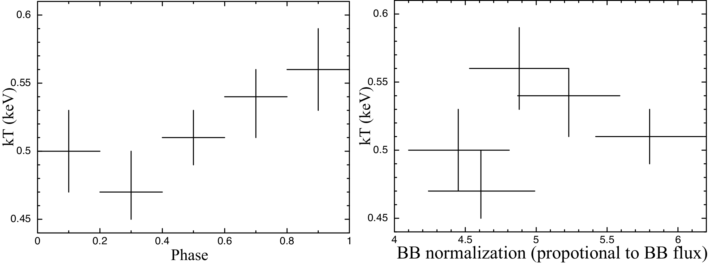
The best-fit parameters of each fitting are presented in Table 3.3. All 14 fittings show acceptable values of . When we fix , we clearly see that the photon index varies among phases beyond their error ranges. Similarly, when we fix , we see that the surface temperature varies among phases beyond their error ranges. These properties are presented in Figure 9 and 10. These results show that the spectrum changes with the pulse phase, which corresponds to the differences in pulse profiles among energies.
Best-fit parameters of the phase-resolved spectral analysis.
∗
∗*
∗
∗*footnotemark:
Phase
†
†{\dagger}
†
†{\dagger}footnotemark:
‡
‡{\ddagger}
‡
‡{\ddagger}footnotemark:
(keV)
BB norm
PL norm
†
†{\dagger}
†
†{\dagger}footnotemark:
(d.o.f.)
0.0–0.5
(fixed)
1.22 (112)
0.5–1.0
(fixed)
1.22 (127)
0.0–0.2
(fixed)
1.43 (43)
0.2–0.4
(fixed)
1.18 (41)
0.4–0.6
(fixed)
0.93 (49)
0.6–0.8
(fixed)
1.25 (53)
0.8–1.0
(fixed)
0.85 (48)
0.0–0.5
(fixed)
1.16 (112)
0.5–1.0
(fixed)
1.24 (127)
0.0–0.2
(fixed)
1.44 (43)
0.2–0.4
(fixed)
1.11 (41)
0.4–0.6
(fixed)
0.92 (49)
0.6–0.8
(fixed)
1.24 (53)
0.8–1.0
(fixed)
0.94 (48)
{tabnote}
∗
∗*
∗
∗*footnotemark:
Only pn and FPMA data are used. Errors denote single-parameter 90% confidence level. The explanations of the parameters are the same as in Table 3.1.3.
†
†{\dagger}
†
†{\dagger}footnotemark:
The offset of the phase is set in accordance with the pulse profiles (Figures 7 and 8).
‡
‡{\ddagger}
‡
‡{\ddagger}footnotemark:
When the parameters are fixed, we adopt the value of the best-fit model of the joint fitting of the average spectrum with XMM-Newton and NuSTAR (see Table 3.1.3). is always fixed to .

4 Discussion
4.1 Broad-band spectra of SGR 1900+14
Our simultaneous broad-band observation with XMM-Newton and NuSTAR successfully measured the spectrum of SGR 1900+14 much more precisely than previous observations. The obtained spectral properties can be compared with those obtained in previous observations performed in the quiescent stages of the object, where bursting activities were not seen.
Table 4.1 presents a comparison of our spectral analysis results with the previous XMM-Newton and Suzaku results in 2005, 2006, and 2009 (Mereghetti et al. 2006; Enoto et al. 2017). We found a clear decrease in the flux of SGR 1900+14, which can be attributed to a continuous decline since the giant flare. We confirm that the 1-10 keV flux decreases by –. The 15–60 keV flux also shows a possible decrease, but this cannot be confirmed because of background model uncertainties of Suzaku HXD (Fukazawa et al. 2009): when we employed the results of another analysis of the same data set (Enoto et al. 2010), the decrease of was not found.
Although the flux shows a clear decrease, the spectral shape does not show significant changes from those observed in 2005, 2006, and 2009. The obtained and values are perfectly matched with those of Suzaku results; they are also comparable with those obtained from the XMM-Newton observations. As for the photon index , our results do not agree with previous studies in terms of XMM-Newton or Suzaku, which is presumably due to the absence of the hard X-ray observation for XMM-Newton and uncertainties of the background model of Suzaku HXD (Fukazawa et al. 2009). Another analysis performed on the same Suzaku observation gives and for the 2006 and 2009 data (Enoto et al. 2010), respectively, both of which agreeing with our result within the errors. Therefore, we suggest that SGR 1900+14 has been quiescent for more than 10 years.
In addition, we found a clear decrease in the 1–60 keV unabsorbed soft component (BB) flux over 10 years. We also found a trend where the PL component may decrease even faster than the BB component because the hardness ratios, which are defined in two ways as or , show decreases, where denotes the 1–60 keV unabsorbed PL flux. However, this result cannot be confirmed because the evaluation of the hardness ratios largely depends on the uncertainties of the HXD background model(Fukazawa et al. 2009).
Comparison of spectral analyses of SGR 1900+14.
Satellite
Date
(keV)
∗
∗*
∗
∗*footnotemark:
∗
∗*
∗
∗*footnotemark:
Abs. HR
†
†{\dagger}
†
†{\dagger}footnotemark:
‡
‡{\ddagger}
‡
‡{\ddagger}footnotemark:
‡
‡{\ddagger}
‡
‡{\ddagger}footnotemark:
HR
†
†{\dagger}
†
†{\dagger}footnotemark:
XMM-Newton
§
§\lx@sectionsign
§
§\lx@sectionsignfootnotemark:
2005-09-20
XMM-Newton
§
§\lx@sectionsign
§
§\lx@sectionsignfootnotemark:
2006-04-01
Suzaku
∥
∥\|
∥
∥\|footnotemark:
2006-04-01
Suzaku
∥
∥\|
∥
∥\|footnotemark:
2009-04-26
XMM+NuSTAR
2016-10-20
{tabnote}
∗
∗*
∗
∗*footnotemark:
Absorbed flux in the 1–10 keV and 15–60 keV energy bands in units of .
†
†{\dagger}
†
†{\dagger}footnotemark:
HR denotes the hardness ratio.
‡
‡{\ddagger}
‡
‡{\ddagger}footnotemark:
and denote 1–60 keV unabsorbed BB and PL flux, respectively, in units of .
§
§\lx@sectionsign
§
§\lx@sectionsignfootnotemark:
The results of analyses are derived from Mereghetti et al. 2006. Because the observation is confined to the soft X-ray range, we cannot obtain information from the hard X-ray range.
∥
∥\|
∥
∥\|footnotemark:
The results of analyses are derived from Enoto et al. 2017.
4.2 Timing properties of SGR 1900+14
4.2.1 Rotation period and its evolution
The detection of coherent pulsation (Section 3.2.2) indicates that the rotation period of SGR 1900+14 was on 2016 October 20 to 23. Figure 11 and Table 4.2.1 present the long-term evolution of the rotation period of SGR 1900+14, where we see a monotonic spin-down over the past 20 years. As shown in Figure 11, the spin-down rate has a large fluctuation. This behavior is typical for magnetars (e.g., CXOU J171405.7-381031: Halpern & Gotthelf 2010; Swift J1822.3-1606: Tong & Xu 2013) and is in clear contrast with the behavior of normal radio pulsars (e.g., the Crab pulsar: Terada et al. 2008).
Here, we define the “post-outburst phase” of SGR 1900+14 as the hatched area in Figure 11. In this phase, the unstable fluctuations of soon after the giant flare (Woods et al. 2002) cease and decreases monotonically. Assuming a constant decay of , we determined a quadratic function (black curve in Figure 11) that describes the trend of in the post-outburst phase. We obtained , which suggests a monotonic decrease in the spin-down rate. shows a drastic decrease from in 2000 April (MJD=51660) to in 2016 October (MJD=57681).
The trend of in the post-outburst phase could be explained by the decrease in the toroidal component (or decrease in the twist) of the magnetic fields in the magnetosphere (twisted magnetosphere model: Thompson et al. 2002; Beloborodov 2009), which is considered to cause a decrease in the spin-down torque. Since the spin-down torque is proportional to the spin-down rate , the observed monotonic decrease in during the post-outburst phase can imply that the twist of the magnetic fields has declined monotonically for more than 15 years since it reached its maximum, which was soon after the giant flare.
Similar behaviors of other magnetars have been reported. For example, PSR J1622-4950, which entered its outburst in or before 2007 June, showed an unstable fluctuation of the spin-down rate soon after its outburst and then a monotonic decrease with a constant rate (Scholz et al. 2017). XTE J1810-197, which is one of the few magnetars that display radio emissions, experienced an outburst in 2003 August along with a subsequent large fluctuation of , which was followed by a slow and gradual decrease of (Pintore et al. 2016). Another example is SGR J1745-2900, which also showed an unstable behavior of soon after its outburst in 2013 April and subsequent gradual monotonic decrease of (Coti Zelati et al. 2015; Coti Zelati et al. 2017). The values of in the post-outburst phases are , , and for PSR J1622-4950, XTE J1810-197, and SGR J1745-2900, respectively. All three values of are negative, as is that for SGR 1900+14, whose is larger than those of the three above-mentioned examples. We point out the possibility that the decay of the twist of magnetic fields in the magnetosphere of SGR 1900+14 has been lasting for more than 15 years, which is much longer than the duration reported for other magnetars. This may be due to the scale of the outburst; we call the outburst of SGR 1900+14 a giant flare with a peak luminosity of , while other magnetars that have such an outburst have peak luminosities of (Anderson et al. 2012; Gotthelf et al. 2004; Coti Zelati et al. 2015). Still, another magnetar SGR 1806-20, which experienced a giant flare and is often regarded as a set with SGR 1900+14, was reported to have a similar trend of the timing evolution (Younes et al. 2015; Younes et al. 2017). It should be noted that since observations have not been conducted so frequently for SGR 1900+14, this is not necessarily the case. For example, the monotonic decrease of may have ceased at some point between 2006 and 2016, where we have no data of the rotation period, and thereafter began linear spin-down behavior like normal radio pulsars.
Employing the newly obtained and , we can evaluate two important parameters: the dipole magnetic field and the characteristic age of SGR 1900+14. These are defined as
| (8) | |||||
| (9) |
The and values on 2016 October 20 give and , respectively. This result means that SGR 1900+14 is older and has a smaller dipole magnetic field than previously reported ( and reported by Olausen & Kaspi 2014 and based on Mereghetti et al. 2006). This is because the previous studies determined these parameters over a short duration without considering the long-term evolution of the rotation period.

List of rotation periods of SGR 1900+14.
Date
(YYYY-MM-DD)
Telescope
Exposure
∗
∗*
∗
∗*footnotemark:
(ks)
(s)
Reference
1996-09-04–1996-09-18
RXTE
47
Marsden et al. 1999
1998-05-31–1998-06-09
RXTE
41.7
Kouveliotou et al. 1999
1998-08-28
RXTE
2.5
Kouveliotou et al. 1999
2000-04-26
RXTE
10
Woods et al. 2002
2001-04-18–2001-05-05
RXTE
128
Woods et al. 2003
2005-09-20
XMM-Newton
47.4
Mereghetti et al. 2006
2006-04-01
XMM-Newton
15.7
Mereghetti et al. 2006
2016-10-20–2016-10-23
NuSTAR
123
This work
{tabnote}
∗
∗*
∗
∗*footnotemark:
If there is a difference in exposure times among detectors, the maximum of them is cited.
4.2.2 Pulse profiles
We found no significant variation in the pulse fraction over 10 years. The pulse profiles obtained with XMM-Newton and NuSTAR all give pulse fractions of 15–20%, which agrees with the previous XMM-Newton observations in 2005 and 2006 (Mereghetti et al. 2006).
The pulse profile shape is almost sinusoidal in the 3–10 keV energy band, while it is more structured in the 10–20 keV. Since the power-law component is dominant in the range 10–20 keV (see Figure 4), we may see contributions of higher multipolar components of the magnetic field on the stellar surface.
4.3 Phase-dependent fluctuation of power-law component
Our phase-resolved spectral analysis (Section 3.3) suggests that the spectral shape varies with the pulse phase. Figure 9 shows the BB temperature as a function of the pulse phase and the relation between the BB temperature and the BB flux, which was obtained with a fixed PL photon index. Although the BB temperature shows variations with the pulse phase, we did not find its correlation with the BB flux, as shown in Figure 9.
As a next step, we explored how the PL component varies with the pulse phase. Figure 10 shows the photon index as a function of the pulse phase and the relation between the photon index and the unabsorbed PL flux. We found a positive correlation between the photon index and the unabsorbed PL flux. Note that although these two parameters can be covariant and positively coupled, we confirmed that the positive correlation is significant by checking their error contours. The relation between the photon index and the PL flux is consistent with the trend of the systematic analysis of various magnetars (Enoto et al. 2010; Enoto et al. 2017). They reported a signature that the hard PL component above 10 keV shows softer spectral photon index as dipole magnetic fields of a magnetar become stronger. This trend was interpreted as a process that the higher magnetic field leads to more photon splittings into lower energy photon, i.e., the softer power-law spectrum.
The positive correlation between the photon index and the PL flux means that the spectrum gets softer when the emitting area, which is usually a hot spot, is better oriented to the observer. We can interpret this trend in terms of photon splitting, which is a nonlinear effect of QED under extremely strong magnetic fields (Baring & Harding 1998; Baring & Harding 2001; Chistyakov et al. 2012). When the PL flux is at the pulse maximum, we can see the region with the strongest magnetic fields, which cause more photon splittings and thus a softer spectrum. Another possibility is that we may see the difference of the path length of splitting photons: the photons from the direction of the magnetic pole travel longer in magnetosphere and experience more splittings. In both cases, our results are consistent with the trend of the photon splitting model.
5 Conclusions
We performed the first simultaneous broad-band observations of the magnetar SGR 1900+14 covering 0.1–78 keV, making full use of the high sensitivity of XMM-Newton and NuSTAR. The NuSTAR hard X-ray coverage enabled us to detect the source up to 70 keV, with a 60–70 keV source significance of .
The spectrum of SGR 1900+14 was well fitted by a typical magnetar spectral model: BB plus PL. We have successfully determined the properties of the spectrum with a higher accuracy than any previous studies, especially for the hard-tail power-law component. The obtained parameters are , , and . We have found that the flux has decreased for more than 10 years, presumably because of the decline from the giant flare, while the spectral shape exhibited no significant variations.
Timing analysis allowed us to determine that the rotation period of SGR 1900+14 on 2016 October 20 to 23 was . The long-term evolution of the rotation period shows a monotonic decrease in in the post-outburst phase, which suggests that the twist of the magnetic fields in the magnetosphere has been decaying for more than 15 years. Its pulse fraction was in the range 15–20%, showing no variation in the past 10 years. The energy-dependent pulse profiles present an interesting trend that the 3–10 keV band is almost perfectly sinusoidal, while the 10–20 keV band contains higher harmonics.
Combining the spectral and temporal analyses, we succeeded in obtaining the phase-resolved spectra. It shows an interesting feature that the photon index and unabsorbed PL flux have a positive correlation, which suggests that we may see differences in the process of photon splitting within one phase cycle.
We thank the anonymous referee for his/her valuable comments. We thank Shinpei Shibata, Kuniaki Masai, Hiromasa Suzuki, Takahiro Matsumoto, and Kazuo Makishima for their helpful advice and discussions. This work was also supported by the Grant-in-Aid for Scientific Research on Innovative Areas “Toward new frontiers: Encounter and synergy of state-of-the-art astronomical detectors and exotic quantum beams” (18H05459; AB). We acknowledge support from JSPS/MEXT KAKENHI grant numbers 18H05459 (AB), 19K03908 (AB), 18H05861 (HO), 16H03954 (HO), 15H00845 (TE), 17K18776 (TE), and 18H04584 (TE).
References
- An et al. (2015) An, H., et al. 2015, ApJ, 807, 93
- Anders & Grevesse (1989) Anders, E., & Grevesse, N. 1989, Geochim. Cosmochim. Acta, 53, 197
- Anderson et al. (2012) Anderson, G. E., et al. 2012, ApJ, 751, 53
- Archibald et al. (2015) Archibald, A. M., et al. 2015, ApJ, 807, 62
- Balucinska-Church & McCammon (1992) Balucinska-Church, M., & McCammon, D. 1992, ApJ, 400, 699
- Baring & Harding (1998) Baring, M. G., & Harding, A. K. 1998, Advances in Space Research, 22, 1121
- Baring & Harding (2001) Baring, M. G., & Harding, A. K. 2001, ApJ, 547, 929
- Beloborodov (2009) Beloborodov, A. M. 2009, ApJ, 703, 1044
- Chistyakov et al. (2012) Chistyakov, M. V., Rumyantsev, D. A., & Stus’, N. S. 2012, Phys. Rev. D, 86, 043007
- Coti Zelati et al. (2015) Coti Zelati, F., et al. 2015, MNRAS, 449, 2685
- Coti Zelati et al. (2017) Coti Zelati, F., et al. 2017, MNRAS, 471, 1819
- Coti Zelati et al. (2018) Coti Zelati, F., Rea, N., Pons, J. A., Campana, S., & Esposito, P. 2018, MNRAS, 474, 961
- Davies et al. (2009) Davies, B., Figer, D. F., Kudritzki, R.-P., Trombley, C., Kouveliotou, C., & Wachter, S. 2009, ApJ, 707, 844
- Enoto et al. (2017) Enoto, T., et al. 2017, ApJS, 231, 8
- Enoto et al. (2010) Enoto, T., Nakazawa, K., Makishima, K., Rea, N., Hurley, K., & Shibata, S. 2010, ApJ, 722, L162
- Esposito et al. (2007) Esposito, P., et al. 2007, A&A, 461, 605
- Feroci et al. (2001) Feroci, M., Hurley, K., Duncan, R. C., & Thompson, C. 2001, ApJ, 549, 1021
- Fukazawa et al. (2009) Fukazawa, Y., et al. 2009, PASJ, 61, S17
- Gonzalez et al. (2010) Gonzalez, M. E., Dib, R., Kaspi, V. M., Woods, P. M., Tam, C. R., & Gavriil, F. P. 2010, ApJ, 716, 1345
- Gotthelf et al. (2004) Gotthelf, E. V., Halpern, J. P., Buxton, M., & Bailyn, C. 2004, ApJ, 605, 368
- Götz et al. (2006) Götz, D., Mereghetti, S., Tiengo, A., & Esposito, P. 2006, A&A, 449, L31
- Halpern & Gotthelf (2010) Halpern, J. P., & Gotthelf, E. V. 2010, ApJ, 725, 1384
- Harding & Lai (2006) Harding, A. K., & Lai, D. 2006, Reports on Progress in Physics, 69, 2631
- Harrison et al. (2013) Harrison, F. A., et al. 2013, ApJ, 770, 103
- Hurley et al. (1999) Hurley, K., et al. 1999, Nature, 397, 41
- Jansen et al. (2001) Jansen, F., et al. 2001, A&A, 365, L1
- Kaspi & Beloborodov (2017) Kaspi, V. M., & Beloborodov, A. M. 2017, ARA&A, 55, 261
- Kouveliotou et al. (1998) Kouveliotou, C., et al. 1998, Nature, 393, 235
- Kouveliotou et al. (1999) Kouveliotou, C., et al. 1999, ApJ, 510, L115
- Madsen et al. (2017) Madsen, K. K., et al. 2017, AJ, 153, 2
- Marsden et al. (1999) Marsden, D., Rothschild, R. E., & Lingenfelter, R. E. 1999, ApJ, 520, L107
- Mazets et al. (1999) Mazets, E. P., Cline, T. L., Aptekar’, R. L., Butterworth, P. S., Frederiks, D. D., Golenetskii, S. V., Il’Inskii, V. N., & Pal’Shin, V. D. 1999, Astronomy Letters, 25, 635
- Mereghetti (2008) Mereghetti, S. 2008, A&A Rev., 15, 225
- Mereghetti et al. (2006) Mereghetti, S., et al. 2006, ApJ, 653, 1423
- Mereghetti & Stella (1995) Mereghetti, S., & Stella, L. 1995, ApJ, 442, L17
- Olausen & Kaspi (2014) Olausen, S. A., & Kaspi, V. M. 2014, VizieR Online Data Catalog, 221
- Pintore et al. (2016) Pintore, F., et al. 2016, MNRAS, 458, 2088
- Scholz et al. (2017) Scholz, P., et al. 2017, ApJ, 841, 126
- Strüder et al. (2001) Strüder, L., et al. 2001, A&A, 365, L18
- Tendulkar et al. (2015) Tendulkar, S. P., et al. 2015, ApJ, 808, 32
- Terada et al. (2008) Terada, Y., et al. 2008, PASJ, 60, S25
- Thompson & Duncan (1995) Thompson, C., & Duncan, R. C. 1995, MNRAS, 275, 255
- Thompson et al. (2002) Thompson, C., Lyutikov, M., & Kulkarni, S. R. 2002, ApJ, 574, 332
- Tong & Xu (2013) Tong, H., & Xu, R.-X. 2013, Research in Astronomy and Astrophysics, 13, 1207-1212
- Tsujimoto et al. (2011) Tsujimoto, M., et al. 2011, A&A, 525, A25
- Turner et al. (2001) Turner, M. J. L., et al. 2001, A&A, 365, L27
- Turolla et al. (2015) Turolla, R., Zane, S., & Watts, A. L. 2015, Reports on Progress in Physics, 78, 116901
- Verner et al. (1996) Verner, D. A., Ferland, G. J., Korista, K. T., & Yakovlev, D. G. 1996, ApJ, 465, 487
- Woods et al. (2002) Woods, P. M., Kouveliotou, C., Gogus, E., Finger, M. H., Swank, J., Markwardt, C. B., & Hurley, K., van der Klis, M. 2002, Neutron Stars in Supernova Remnants, 271, 313
- Woods et al. (2003) Woods, P. M., et al. 2003, ApJ, 596, 464
- Younes et al. (2017) Younes, G., et al. 2017, ApJ, 851, 17
- Younes et al. (2015) Younes, G., Kouveliotou, C., & Kaspi, V. M. 2015, ApJ, 809, 165