跳到论文正文
W Papers独立论文阅读器 arXiv:1906.04396 论文正文 计算阅读时间 · 0%
引用这篇论文根据当前论文元数据生成,正式投稿前建议核对。


License: arXiv.org perpetual non-exclusive license
arXiv:1906.04396v1 [math.ST] 11 Jun 2019

Detection and estimation of parameters in high dimensional multiple change point regression models via ℓ1/ℓ0\ell_{1}\big/\ell_{0} regularization and discrete optimization
Abhishek Kaula,aa a Address for correspondence: Abhishek Kaul, Department of Mathematics and Statistics, Washington State University, Pullman, WA 99164, USA. Email: abhishek.kaul@wsu.edu., Venkata K. Jandhyalaa, Stergios B. Fotopoulosb

aDepartment of Mathematics and Statistics, bDepartment of Finance and Management Science, Washington State University, Pullman, WA 99164, USA.

Keywords: Multiple change points, Multiphase regression, High dimensional regression, ℓ1,\ell_{1}, ℓ0\ell_{0} regularization, Simulated annealing.

Abstract

Binary segmentation, which is sequential in nature is thus far the most widely used method for identifying multiple change points in statistical models. Here we propose a top down methodology called arbitrary segmentation that proceeds in a conceptually reverse manner. We begin with an arbitrary superset of the parametric space of the change points, and locate unknown change points by suitably filtering this space down. Critically, we reframe the problem as that of variable selection in the change point parameters, this enables the filtering down process to be achieved in a single step with the aid of an ℓ0\ell_{0} regularization, thus avoiding the sequentiality of binary segmentation. We study this method under a high dimensional multiple change point linear regression model and show that rates convergence of the error in the regression and change point estimates are near optimal. We propose a simulated annealing (SA) approach to implement a key finite state space discrete optimization that arises in our method. Theoretical results are numerically supported via simulations. The proposed method is shown to possess the ability to agnostically detect the ‘no change’ scenario. Furthermore, its computational complexity is of order O⁡(N​p2)+SA,O(Np^{2})+{\rm SA}, where SA is the cost of a SA optimization on a NN (no. of change points) dimensional grid. Thus, the proposed methodology is significantly more computationally efficient than existing approaches. Finally, our theoretical results are obtained under weaker model conditions than those assumed in the current literature.

1 Introduction

High dimensional regression models that allow vastly larger number of parameters pp than the sample size n,n, have found applications in many fields of scientific inquiry such as genomics, social networking, empirical economics, finance among many others. This has led to a rapid development of statistical literature investigating methods capable of analyzing such models and data sets. One of the most successful methods for analysing high dimensional regression models has been the Lasso, which is based on the least squares loss and ℓ1\ell_{1} regularization (Tibshirani, 1996). Innumerable investigations have since been carried out to study the behavior of the Lasso estimator and its various modifications in many different settings (see e.g., Zou, 2006; Zhao & Yu, 2006; Bickel et al. , 2009; Belloni et al. , 2011 Belloni et al. , 2017b; Kaul, 2014, Kaul & Koul, 2015 and the references therein). For a general overview on the developments of Lasso and its variants we refer to the monograph of Bühlmann & Van De Geer, 2011 and the review article of Tibshirani, 2011. All aforementioned articles provide results in a regression setting where the parameters are dynamically stable. In contrast, multiphase/change point regression models provide a dynamic setting in which regression parameters are allowed to switch values based on a change inducing variable or in a time ordered sense. Such models allow for a greater versatility in modelling data, especially in a high dimensional setting. In many experiments, the estimated locations of change points may reveal additional critical information of interest.

In the past few years several articles have studied high dimensional change point models in an ‘only means’ setup. In this setting, change points are characterized with respect to dynamic mean vectors of time ordered random vectors, where the dimension of the observation vector may be larger than the number of observations (Cho & Fryzlewicz, 2015, Fryzlewicz, 2014,and Wang & Samworth, 2018; among others). Another context in which high dimensional change point models have been investigated is that of a dynamic covariance structure which is related to the study of evolving networks (Roy et al. , 2017,Gibberd & Roy, 2017, Atchade & Bybee, 2017; among others). In contrast, change point methods for high dimensional linear regression models have received much less attention and only a select few articles have considered this problem in the recent literature.

In this paper, we consider a high dimensional multiphase (change point) regression model given by,

yi=∑j=1N+1xiTβ(j−1)0𝟏[τj−10<wi≤τj0]+εi,i=1,..,n,\displaystyle y_{i}=\sum_{j=1}^{N+1}x_{i}^{T}\beta_{(j-1)}^{0}{\bf 1}[\tau_{j-1}^{0}<w_{i}\leq\tau_{j}^{0}]+\varepsilon_{i},\quad i=1,..,n, (1.1)

where N≥0,N\geq 0, τ00=−∞,\tau_{0}^{0}=-\infty, τN+10=∞,\tau_{N+1}^{0}=\infty, and 𝟏​[⋅]{\bf 1}[\cdot] represents the indicator function. The components of the change point parameter vector are assumed to be τ0=(τ10,…,τN0)T∈ℝ¯N,\tau^{0}=(\tau^{0}_{1},...,\tau^{0}_{N})^{T}\in\bar{\mathbb{R}}^{N}, ℝ¯=ℝ∪{−∞}\bar{\mathbb{R}}={\mathbb{R}}\cup\{-\infty\} such that τj−10≤τj0,\tau_{j-1}^{0}\leq\tau_{j}^{0}, j=1,…,N.j=1,...,N. First note that when τ0=τ10=…=τN0=−∞,\tau_{0}=\tau_{1}^{0}=...=\tau_{N}^{0}=-\infty, model (1.1) reduces to an ordinary linear regression model without change points. This case where all change points are at negative infinity characterizes the case of ‘no change’, and in the following we refer to this case as N=0.N=0. On the other hand we characterize the case of one or more change points, N≥1,N\geq 1, as when the components of τ0\tau^{0} are distinct and finite, i.e., −∞<τ10<…<τN0.-\infty<\tau^{0}_{1}<...<\tau^{0}_{N}. The observed variables in model (1.1) are the response yi∈ℝ,y_{i}\in{\mathbb{R}}, the pp-dimensional predictors xi∈ℝp,x_{i}\in{\mathbb{R}}^{p}, and change inducing variable wi∈ℝ.w_{i}\in{\mathbb{R}}. The parameters of interest are the number of change points N∈{0,1,2,…},N\in\{0,1,2,...\}, the change point parameter vector τ0∈ℝ¯N,\tau^{0}\in\bar{\mathbb{R}}^{N}, and the regression parameters β(j)0∈ℝp,\beta_{(j)}^{0}\in{\mathbb{R}}^{p}, j=0,…,N.j=0,...,N. The change points τj0\tau_{j}^{0} j=1,..,Nj=1,..,N represents threshold values of the variable ww subsequent to which the regression parameter changes from its current value β(j−1)\beta_{(j-1)} to a new value β(j).\beta_{(j)}. Furthermore, we let p>>n,p>>n, so that model (1.1) corresponds to a high dimensional setting.

In the classical setting with a fixed number of parameters and n→∞,n\to\infty, change point regression models such as (1.1) have been extensively investigated, albeit a large proportion of this literature is developed in the case with only a single change point. The works of Hinkley, 1970, Hinkley, 1972, Jandhyala & MacNeill, 1997, Bai, 1997, Jandhyala & Fotopoulos, 1999, and Jandhyala et al. , 2013, investigate the setting where parameters are assumed to change at certain unknown time points of the sampling period. On the other hand, the works of Hinkley, 1969, Koul & Qian, 2002, and Koul et al. , 2003 study the setting where the change point is formulated based on one or more covariate thresholds. In the literature, the latter approach is typically referred to as two-phase or multiphase regression, however it is also common to broadly call both as change point regression models.

The literature on regularized estimation in change point regression models is very sparse. Models similar to (1.1) with a single change point have been studied by Kaul et al. , 2019, Lee et al. , 2016, and Lee et al. , 2018 in the high dimensional setting. The case of multiple change points is investigated in Ciuperca, 2014, Zhang et al. , 2015, , Jin et al. , 2016 and Leonardi & Bühlmann, 2016. Amongst these articles the first three consider the fixed pp setting, whereas the last article considers the high dimensional setting as is also the case in this paper. The article of Leonardi & Bühlmann, 2016 proposes a binary segmentation approach for the recovery of change points of the regression model, where change points are searched for, and then added to the set of all change points one by one. In the context of change point parameters, this binary segmentation approach can be viewed as the counterpart of step-up regression where parameters are included sequentially. It is important to remember that in the current high dimensional setting, in order to search for a single change point for each segment, the approach of Leonardi & Bühlmann, 2016 requires O⁡(n​Lasso​(n))O\big(n{\rm Lasso}(n)\big) computations, where Lasso(n)(n) represents the computational cost of running one Lasso optimization with a sample size n.n. In fact the authors show that the overall computation cost of their approach is of the order O(n​log⁡(n)n\log(n)Lasso(n)(n)).

In contrast, our approach proceeds in a conceptually reverse manner. The method that we propose can be viewed in a sense as the counterpart of step-down regression for the change point parameters. We begin with a superset of the parameteric space of the unknown change points and filter this space down to identify the unknown change points, following which we estimate the regression parameters. Critically, the ‘stepping down’ process in our methodology can be carried out in a single step via a ℓ0\ell_{0} regularization. We achieve this by converting the problem of recovery of change points to a variable selection problem in the change point parameters. This conversion of the change point estimation problem to a variable selection problem in turn relies on initial regression estimates. The second main novelty of this manuscript is to show that, initial regression estimates that are much slower than optimal in rates of convergence can be utilized to obtain change point estimates that are themselves near optimal in rates of convergence. In other words, our setup constitutes a rare statistical scenario where relatively ‘poor’ estimates of some parameters of a model can be utilized to obtain near optimal estimates of other parameters of the model.

The proposed method circumvents the sequential approach of binary segmentation for the recovery of change points. Consequently, the method requires only Lasso(n)+(n)+SA computations for the identification and recovery of change points, where SA represents the computational cost of a simulated annealing optimization which is typically very efficient. The simulated annealing algorithm is used to implement a key discrete optimization over an O⁡(N)O(N) dimensional space that arises in our methodology due to the use of an ℓ0\ell_{0} regularization. Thus our approach is far more efficient than any existing comparable methodology for high dimensional change point regression models. Being based on a ℓ0\ell_{0} regularization, our approach also provides the ability to detect the case of N=0,N=0, where an ordinary linear regression without change points is more appropriate. In comparison, binary segmentation approaches typically require the existence of at least one change point. Finally, we also note that our analysis requires significantly weaker assumptions than those currently assumed in the literature. Further comparisons of our method, assumptions and results with the existing literature are made in Section 2.

The remainder of this article is organized as follows. Section 2 provides the proposed methodology and technical assumptions required for the theoretical analysis. Section 3 provides the main theoretical results regarding the performance of the proposed methodology. Section 4 discusses the implementation of the proposed method and a simulated annealing approach for the implementation of a key step of our method. This section also provides numerical results on the finite sample performance of our method. The proofs of all main results are provided in Appendix A of the Supplementary materials of this article. Some additional technical results and lemma’s are provided in Appendix B of the Supplementary materials.

Notations: We conclude this section with a short note on the notations used in this paper. Throughout the paper, for any vector δ∈ℝp,\delta\in{\mathbb{R}}^{p}, ‖δ‖0\|\delta\|_{0} represents the number of non-zero components in δ,\delta, and ‖δ‖1\|\delta\|_{1} and ‖δ‖2\|\delta\|_{2} represent the usual 11-norm and Euclidean norm, respectively. The norm ‖δ‖∞\|\delta\|_{\infty} represents the usual sup norm, i.e., the maximum of absolute values of all elements. For any set of indices S⊆{1,….,p},S\subseteq\{1,....,p\}, let δS=(δj)j∈S\delta_{S}=(\delta_{j})_{j\in S} represent a sub-vector of δ\delta containing components corresponding to the indices in S.S. Also, let |S||S| represent the cardinality of the set S.S. The notation 𝟏​[⋅]{\bf 1}[\cdotp] represents the usual indicator function. We denote by Φ⁡(⋅)\Phi(\cdotp) the cdf of wi′w_{i}^{\prime}s and let d⁡(τa,τb)=P⁡(τa<wi≤τb)=Φ⁡(τb)−Φ⁡(τa),d(\tau_{a},\tau_{b})=P(\tau_{a}<w_{i}\leq\tau_{b})=\Phi(\tau_{b})-\Phi(\tau_{a}), τa≤τb∈ℝ¯,\tau_{a}\leq\tau_{b}\in\bar{\mathbb{R}}, clearly, d⁡(τa,τb)=0⇔τa=τb.d(\tau_{a},\tau_{b})=0\Leftrightarrow\tau_{a}=\tau_{b}. We represent by ℝ¯=ℝ∪{−∞}\bar{\mathbb{R}}={\mathbb{R}}\cup\{-\infty\} as the extended Euclidean space, with only the left closure point included. We shall also use the notation a∨b=max⁡{a,b},a\vee b=\max\{a,b\}, and a∧b=min⁡{a,b},a\wedge b=\min\{a,b\}, a,b∈ℝ.a,b\in{\mathbb{R}}. The notation cu,cmc_{u},c_{m} is used to represent generic constants that may be different from one line to the next. Here, 0<cu<∞0<c_{u}<\infty represent universal constants, whereas 0<cm<∞0<c_{m}<\infty are constants that depend on model parameters such as variance parameters of underlying distributions. Lastly, 0<c1,c2<∞0<c_{1},c_{2}<\infty are also generic constants that may depend on both cu,c_{u}, and cm.c_{m}.

2 Methodology and Related Work

2.1 Proposed methodology

For any τa,τb∈ℝ¯,\tau_{a},\tau_{b}\in\bar{\mathbb{R}}, τa≤τb\tau_{a}\leq\tau_{b} and any γ∈ℝp,\gamma\in{\mathbb{R}}^{p}, define the segmentwise least squares loss as,

Q∗(γ,τa,τb):=∑i=1n(yi−xiTγ)2𝟏[τa<wi≤τb],\displaystyle Q^{*}(\gamma,\tau_{a},\tau_{b}):=\sum_{i=1}^{n}(y_{i}-x_{i}^{T}\gamma)^{2}{\bf 1}[\tau_{a}<w_{i}\leq\tau_{b}], (2.1)

where the indicator function 𝟏[τa<wi≤τb]=0{\bf 1}[\tau_{a}<w_{i}\leq\tau_{b}]=0bb b This is a slight misuse of notation, and is only used for simpler exposition. To be notationally precise, this term should be 𝟏[wi≤τb]−𝟏[wi≤τa]{\bf 1}[w_{i}\leq\tau_{b}]-{\bf 1}[w_{i}\leq\tau_{a}], for τa≤τb\tau_{a}\leq\tau_{b} if τa=τb.\tau_{a}=\tau_{b}. For any Nˇ≥1,\check{N}\geq 1, let τˇ:=(τˇ1,…,τˇNˇ)T∈ℝ¯Nˇ,\check{\tau}:=(\check{\tau}_{1},...,\check{\tau}_{\check{N}})^{T}\in\bar{\mathbb{R}}^{\check{N}}, be any vector such that τˇj−1≤τˇj,\check{\tau}_{j-1}\leq\check{\tau}_{j}, j=1,…,Nˇ,j=1,...,\check{N}, τˇ0=−∞.\check{\tau}_{0}=-\infty. Also, let τˇN+1=∞\check{\tau}_{N+1}=\infty such that (τˇ0,τˇT,τˇNˇ+1)T(\check{\tau}_{0},\check{\tau}^{T},\check{\tau}_{\check{N}+1})^{T} forms a partition of ℝ¯.\bar{\mathbb{R}}. Additionally, for any sequence of vectors α(j)∈ℝp,\alpha_{(j)}\in{\mathbb{R}}^{p}, j=0,…,Nˇj=0,...,\check{N} denote by α=(α(0)T,….,α(Nˇ)T)T∈ℝ(Nˇ+1)​p\alpha=(\alpha_{(0)}^{T},....,\alpha_{(\check{N})}^{T})^{T}\in{\mathbb{R}}^{{(\check{N}+1)}p} as the concatenation of all α(j)​s.\alpha_{(j)}s. Then define the total least squares loss evaluated at (Nˇ,α,τˇ)(\check{N},\alpha,\check{\tau}) as,

Q⁡(Nˇ,α,τˇ):=1n​∑j=1Nˇ+1Q∗​(α(j−1),τˇj−1,τˇj).\displaystyle Q(\check{N},\alpha,\check{\tau}):=\frac{1}{n}\sum_{j=1}^{\check{N}+1}Q^{*}(\alpha_{(j-1)},\check{\tau}_{j-1},\check{\tau}_{j}).

Next, for any τ∈ℝNˇ,\tau\in{\mathbb{R}}^{\check{N}}, define 𝒯^​(τ)⊆{1,…,Nˇ}\hat{\cal T}(\tau)\subseteq\{1,...,\check{N}\} as the set of indices of distinct and finite components of τ,\tau, i.e.,

𝒯^​(τ)={j∈{1,…,Nˇ};τj−1≠τj,τj≠−∞},\displaystyle\hat{\cal T}(\tau)=\big\{j\in\{1,...,\check{N}\}\,\,;\,\,\tau_{j-1}\neq\tau_{j},\,\,\tau_{j}\neq-\infty\big\}, (2.2)

where τ0=−∞.\tau_{0}=-\infty. Under these notations and the model (1.1), we propose estimators for the number of change points, locations of change points and the regression coefficients respectively. These estimators are stated in the following as two algorithms each consisting of two steps. The first algorithm is designed to recover the number and locations of change points of the model (1.1) and the second to recover the corresponding regression coefficients. All technical assumptions required for the theoretical validity of the proposed estimates are stated in Section 2.2.


Algorithm 1: Estimation of number and locations of change point(s)

 
  • Step 0:

    (Initializing step) Choose any Nˇ≥1∨N,\check{N}\geq 1\vee N, and any vector τˇ=(τˇ1,…,τˇNˇ)T∈ℝNˇ,\check{\tau}=(\check{\tau}_{1},...,\check{\tau}_{\check{N}})^{T}\in{\mathbb{R}}^{\check{N}}, satisfying Condition A. Compute initial regression estimates α^(j),\hat{\alpha}_{(j)}, for each j=0,…,Nˇ,j=0,...,\check{N},

    α^(j)=arg​minα∈ℝp⁡{1n​Q∗​(α,τˇj−1,τˇj)+λ0​‖α‖1},λ0>0\displaystyle\hat{\alpha}_{(j)}=\argmin_{\alpha\in{\mathbb{R}}^{p}}\Big\{\frac{1}{n}Q^{*}(\alpha,\check{\tau}_{j-1},\check{\tau}_{j})+\lambda_{0}\|\alpha\|_{1}\Big\},\qquad\lambda_{0}>0
  • Step 1:

    Update τˇ∈ℝNˇ\check{\tau}\in{\mathbb{R}}^{\check{N}} to obtain estimate τ^∈ℝ¯Nˇ\hat{\tau}\in\bar{\mathbb{R}}^{\check{N}}, wherecc c Note that while the initializing τˇ\check{\tau} in Step 0 is chosen in ℝNˇ,{\mathbb{R}}^{\check{N}}, however the optimization in Step 1 is performed over the extended Euclidean space ℝ¯Nˇ.\bar{\mathbb{R}}^{\check{N}}.,

    τ^=arg​minτ∈ℝ¯Nˇ;τj−1≤τj​∀j⁡{Q⁡(Nˇ,α^,τ)+μ​∑j=1Nˇ‖d⁡(τj−1,τj)‖0},μ>0\displaystyle\hat{\tau}=\argmin_{\begin{subarray}{c}\tau\in\bar{\mathbb{R}}^{\check{N}};\\ \tau_{j-1}\leq\tau_{j}\,\forall\,j\end{subarray}}\Big\{Q(\check{N},\hat{\alpha},\tau)+\mu\sum_{j=1}^{\check{N}}\|d(\tau_{j-1},\tau_{j})\|_{0}\Big\},\qquad\mu>0

    Let 𝒯^:=𝒯^​(τ^),\hat{\cal T}:=\hat{\cal T}(\hat{\tau}), and update the estimated number of change points to N~=|𝒯^|,\tilde{N}=|\hat{\cal T}|, and recover the corresponding locations of change points as the subset τ~=τ^𝒯^∈ℝN~.\tilde{\tau}=\hat{\tau}_{\hat{\cal T}}\in{\mathbb{R}}^{\tilde{N}}.


Algorithm 1 begins (Step 0) with a nearly arbitrary partition τˇ\check{\tau} in a superset ℝNˇ{\mathbb{R}}^{\check{N}} of the parametric space ℝN{\mathbb{R}}^{N} of the unknown change points. The simple update in Step 1 of Algorithm 1 recovers the number of change points N~,\tilde{N}, and the corresponding locations τ~.\tilde{\tau}. There are two main novelties of Algorithm 1. First, instead of searching for change points sequentially, Algorithm 1 searches for them in a larger parametric space by reframing the problem as one of variable selection. Here the selection is in terms of differences between adjacent τj\tau_{j}’s, i.e., the ℓ0\ell_{0} regularization in Step 1 is forcing these adjacent components to collapse towards each other. This regularization can be viewed as a ℓ0\ell_{0} version of the total variation penalty on the components τ.\tau. The second main novelty is that in order to achieve this conversion to a variable selection problem, we use a nearly arbitrary partition that serves as an initial rough guess. It shall become theoretically and empirically apparent in the following that the estimates obtained in Step 1 are robust against this initial partition, i.e., nearly any arbitrarily chosen partition in Step 0 shall yield near optimal estimates from Step 1. The underlying working mechanism of Algorithm 1 is illustrated in Figure 1.

Step 0−∞-\inftyτ10\tau_{1}^{0}τ20\tau_{2}^{0}τˇ1\check{\tau}_{1}τˇ2\check{\tau}_{2}τˇ3\check{\tau}_{3}τˇ4\check{\tau}_{4}τˇ5\check{\tau}_{5}∞\inftyα^(0)\hat{\alpha}_{(0)}α^(1)\hat{\alpha}_{(1)}α^(2)\hat{\alpha}_{(2)}α^(3)\hat{\alpha}_{(3)}α^(4)\hat{\alpha}_{(4)}α^(5)\hat{\alpha}_{(5)}Step 1−∞-\inftyτ^2\hat{\tau}_{2}τ^4\hat{\tau}_{4}∞\infty
Figure 1: Illustration of the working mechanism of Algorithm 1 with N=2,N=2, Nˇ=5\check{N}=5: Initializing with a nearly arbitrary partition τˇ=(τˇ1,…,τˇ5)T\check{\tau}=(\check{\tau}_{1},...,\check{\tau}_{5})^{T} and corresponding regression coefficient estimates α^(j),\hat{\alpha}_{(j)}, j=0,..,5,j=0,..,5, the algorithm converges to the unknown number of change points and the locations of the distinct change points lie in an optimal neighborhood of the unknown change points. Specifically, the components nearest to an unknown τj0\tau^{0}_{j} shall converge toward it, and all remaining components converge either to the previous or the next component.

Next, we propose Algorithm 2 for the estimation of regression parameter vectors of model (1.1). This algorithm utilizes the estimated number (N~\tilde{N}) and locations (τ~\tilde{\tau}) of change points from Algorithm 1, to obtain coefficient estimates on the corresponding partition yielded by τ~.\tilde{\tau}. Note that when N~=0\tilde{N}=0 from Algorithm 1, then Algorithm 2 is equivalent to implementing the ordinary Lasso on the data (xi,yi),(x_{i},y_{i}), i=1,…,n.i=1,...,n.


Algorithm 2: Estimation of regression coefficients

 
  • Step 0:

    Compute N~\tilde{N} and τ~\tilde{\tau} from Algorithm 1. If N~=0,\tilde{N}=0, then fit a linear regression model without change points via Lasso.

  • Step 1:

    If N~≥1,\tilde{N}\geq 1, then for each j=0,…,N~,j=0,...,\tilde{N}, update regression parameter estimates,

    α~(j)=arg​minα∈ℝp⁡{1n​Q∗​(α,τ~j−1,τ~j)+λ1​j​‖α‖1},λ1​j>0.\displaystyle\tilde{\alpha}_{(j)}=\argmin_{\alpha\in{\mathbb{R}}^{p}}\Big\{\frac{1}{n}Q^{*}(\alpha,\tilde{\tau}_{j-1},\tilde{\tau}_{j})+\lambda_{1j}\|\alpha\|_{1}\Big\},\qquad\lambda_{1j}>0.
 

The main theoretical contribution of this manuscript is to show that the proposed methodology consistently recovers the unknown number of change points, and yields estimates of the locations of change points and that of regression coefficient vectors that are near optimal in their rates of convergence. Specifically, under suitable conditions, we shall derive the following relations that hold for nn sufficiently large with probability at least 1−c1​(1∨N)​exp⁡(−c2​log⁡p).1-c_{1}(1\vee N)\exp(-c_{2}\log p).

(i)\displaystyle(i) When​N≥0,N~=N,\displaystyle\,\,{\rm When}\,\,N\geq 0,\quad\tilde{N}=N, (2.3)
(i​i)\displaystyle(ii) WhenN≥1,∑j=1Nd(τ~j,τj0)≤cucmNs​log⁡pn,and\displaystyle\,\,{\rm When}\,\,N\geq 1,\quad\sum_{j=1}^{N}d(\tilde{\tau}_{j},\tau^{0}_{j})\leq c_{u}c_{m}N\frac{s\log p}{n},\,\,{\rm and}
(i​i​i)\displaystyle(iii) ∑j=0N∥α~(j)−β0(j)∥q≤cucmNs1qlog⁡pn,q=1,2.\displaystyle\sum_{j=0}^{N}\|\tilde{\alpha}_{(j)}-\beta^{0}_{(j)}\|_{q}\leq c_{u}c_{m}Ns^{\frac{1}{q}}\sqrt{\frac{\log p}{n}},\quad q=1,2.

In an ordinary high dimensional linear regression model without change points, it has been shown that the optimal rate of convergence for a regression parameter vector estimate is s​log⁡p/n\sqrt{s\log p/n} under the ℓ2\ell_{2} norm (Ye & Zhang, 2010, Raskutti et al. , 2011, Belloni et al. , 2017a). Also, the rate of convergence of the change point estimates in (2.3) matches the fastest available in the literature, see, e.g., (Kaul et al. , 2019, Lee et al. , 2016, Leonardi & Bühlmann, 2016, Lee et al. , 2018).

The result in (2.3) is quite surprising since the estimates N~\tilde{N} and τ~\tilde{\tau} are computed based on initial regression coefficient estimates α^\hat{\alpha} from Step 0 of Algorithm 1. These regression estimates may not be anywhere near optimal in their rate of convergence, since these are in turn computed based on a nearly arbitrary partition of the support of w.w. Despite these rough regression estimates, we can prove that Step 1 of Algorithm 1 identifies the change points correctly and provides estimates that are indeed near optimal in their rate of convergence.

Next, we discuss two immediate concerns that may arise to the reader regarding Algorithm 1. First, how stringent is Condition A on the initializers Nˇ\check{N} and τˇ\check{\tau} in Step 0 of this algorithm. This condition on the initializers is infact very mild. For Algorithm 1, where Nˇ\check{N} is user chosen, nearly any arbitrarily chosen partition with a large enough Nˇ≥1∨N,\check{N}\geq 1\vee N, satisfies this condition. Other requirements of this condition are only meant to remove pathological cases, such as when all components of τˇ\check{\tau} are closely clustered together or are concentrated at one end of the support of w.w. From a practical perspective, an equally spaced large enough partition, as expected, works well in all empirically examined cases.

A second concern that may arise regarding Algorithm 1 is whether the optimization of Step 1 of these methods is computationally feasible. At first impression, the optimization of Step 1 does indeed appear to be computationally intensive given that it is a nonsmooth, nonconvex optimization (with no apparent convex relaxations), and with potentially multiple global optimums. However the following observations shall serve to erase this impression. Note that although this optimization of Step 1 is over the extended Euclidean space ℝ¯Nˇ,\bar{\mathbb{R}}^{\check{N}}, however, the loss function Q(Nˇ,α^,⋅)Q(\check{N},\hat{\alpha},\cdotp) is a step function over the finite grid τ∈{−∞,w1,….,wn}Nˇ,\tau\in\{-\infty,w_{1},....,w_{n}\}^{\check{N}}, with step change occurring at grid points on this Nˇ\check{N} dimensional grid (see, Figure 3 in Section 4 for an illustration of this behavior). Additionally, the ℓ0\ell_{0} norm term in the optimization of Step 1 is either 00 or 1,1, based on whether τj−1\tau_{j-1} and τj\tau_{j} are equal or unequal respectively, in other words the distance between τj−1\tau_{j-1} and τj\tau_{j} does not influence the value of ℓ0\ell_{0} norm (note that this will not be true if in Step 1, the ℓ1\ell_{1} norm is considered in place of the ℓ0\ell_{0} norm). These two observations together imply that any global optimum achieved in the extended Euclidean space ℝ¯Nˇ\bar{\mathbb{R}}^{\check{N}} is also attained at some Nˇ\check{N} dimensional point on the grid {−∞,w1,….,wn}Nˇ.\{-\infty,w_{1},....,w_{n}\}^{\check{N}}. In other words, the optimization in Step 1 is reduced to a discrete optimization on a finite state space (the total number of possible states being (n+1)Nˇ(n+1)^{\check{N}}). In view of these observations, the optimization in Step 1 is reminiscent of the well known travelling salesman problem, and correspondingly can be solved efficiently using a simulated annealing approach. Additionally, since simulated annealing is not a gradient based approach, it is capable of easily handling a ℓ0\ell_{0} penalty. A detailed discussion of the implementation of Algorithm 1 is provided in Section 4. We also note that Step 0 of Algorithm 1, and Step 1 of Algorithm 2 are Lasso(n,p)\big(n,p\big) estimates. Thereby, these two steps are efficiently implementable using any one of the several available methods in the literature, for e.g. coordinate or gradient descent algorithms, see, e.g. Hastie et al. , 2015 or via interior point methods for linear optimization under second order conic constraints, see, e.g., Koenker & Mizera, 2014.

Finally, we conclude this section by also emphasizing the computational efficiency of the proposed Algorithm 1. First note that Step 0 of Algorithm 1 are (Nˇ+1)(\check{N}+1) computations of Lasso(n,p)(n,p) estimates. It is also known that computational complexity of most algorithms for the Lasso optimization scales like O⁡(p2).O(p^{2}). As briefly described above, Step 1 of Algorithm 1 shall be implemented via simulated annealing (SA) over a Nˇ\check{N} dimensional grid. SA optimizations are known to be very efficient for a large class of problems and can ordinarily be accomplished in a time scaling of order O⁡(Nˇ4),O(\check{N}^{4}), see, e.g. Sasaki, 1987. We also mention that in the worst case the complexity of SA can also be exponential, depending on the optimization under consideration. However, in our study the SA optimization of Step 1 is empirically observed to be well behaved and carried out with a cheap computational cost. Thus, assuming Nˇ≤c⁡(1∨N),\check{N}\leq c(1\vee N), c≥1,c\geq 1, the overall complexity of Algorithm 1 is O⁡((1∨N)​p2)+S​A.O\big((1\vee N)p^{2}\big)+SA. Thereby, this algorithm is far more computationally efficient than any comparable existing method for the estimation of parameters of model (1.1). To see this, compare the above complexity to the binary segmentation approach proposed in Leonardi & Bühlmann, 2016. They show that the their method is implementable with O⁡(n​log⁡n)O(n\log n)Lasso(n,(N+1)​p)\big(n,(N+1)p\Big) computations with the aid of dynamic programming, thus the procedure effectively yields a time scaling of O⁡(n​N​p2).O(nNp^{2}).

2.2 Assumptions

In this subsection we state all necessary conditions and technical assumptions under which the results of this article are derived.

Condition A (requirements of initializer):
 (i) The initializing vector τˇ=(τˇ1,….,τˇNˇ)T∈ℝNˇ\check{\tau}=(\check{\tau}_{1},....,\check{\tau}_{\check{N}})^{T}\in{\mathbb{R}}^{\check{N}} is such that Nˇ\check{N} is larger than the true number of change points, i.e., Nˇ≥1∨N,\check{N}\geq 1\vee N, and Nˇ≤cu​(1∨N),\check{N}\leq c_{u}(1\vee N), cu≥1.c_{u}\geq 1.
  (ii) All initial change points are sufficiently separated, i.e., d⁡(τˇj−1,τˇj)>lmin>0,d(\check{\tau}_{j-1},\check{\tau}_{j})>l_{\min}>0, for all j=1,…,Nˇ+1,j=1,...,\check{N}+1, for some positive sequence lmin,l_{\min}, where τˇ0,τˇNˇ+1\check{\tau}_{0},\check{\tau}_{\check{N}+1} denote −∞-\infty and ∞\infty respectively.
  (iii) Let uˇn=1∨cu​(1/n)1/k,{\check{u}}_{n}=1\vee c_{u}(1/n)^{1/k}, for some constants k∈[1,∞),k\in[1,\infty), and cu>0.c_{u}>0. Then assume that there exists a subset 𝒯:={m0,m1,…,mN,mN+1}⊆{0,1,2,….Nˇ+1}{\cal T}:=\{m_{0},m_{1},...,m_{N},m_{N+1}\}\subseteq\{0,1,2,....\check{N}+1\} such that m0=0,m_{0}=0, mN+1=Nˇ+1m_{N+1}=\check{N}+1 and max1≤j≤N⁡d⁡(τˇmj,τj0)≤uˇn.\max_{1\leq j\leq N}d(\check{\tau}_{m_{j}},\tau^{0}_{j})\leq{\check{u}}_{n}. When N=0,N=0, define 𝒯:={m0,mN+1}.{\cal T}:=\{m_{0},m_{N+1}\}.

As briefly discussed earlier, Condition A is a mild assumption on the initializers. Roughly speaking, this condition requires the initial change point vector to be a large enough partition of ℝ{\mathbb{R}} where the components of this initializing vector are sufficiently separated from each other. Also, this condition requires that at least one initial change point lies in some fractional neighborhood of each unknown change point. The condition d⁡(τˇmj,τj0)≤uˇn,d(\check{\tau}_{m_{j}},\tau^{0}_{j})\leq{\check{u}}_{n}, j=1,…,Nj=1,...,N is very mild since the constant kk can be arbitrarily largedd d The constant kk can be arbitrarily large as long as the rate conditions of Condition B and C are satisfied.. In one of our main results, we shall show that despite the initializers τˇmj\check{\tau}_{m_{j}} lying in an arbitrary fractional neighborhood of τj0,\tau_{j}^{0}, the updated change point estimate τ~\tilde{\tau} satisfies ‖τ~−τ0‖1≤N​s​log⁡p/n,\|\tilde{\tau}-\tau^{0}\|_{1}\leq Ns\log p/n, with high probability. Note that, the localization error bound of τ~\tilde{\tau} is free of k.k. This condition is similar to Condition I assumed in Kaul et al. , 2019, we refer to that article for further insights on this condition. Here we also state that implementation of the proposed methodology does not require prior knowledge of k.k.

It is observed a large enough grid of equally separated initial change points works well in nearly all empirically examined cases. The term lminl_{\min} in Condition A(i) is allowed to potentially decrease to zero with n,n, however this dependence is suppressed for clarity of exposition. The rate at which such a convergence of lminl_{\min} is allowed also depends on other model parameters, and is explicitly stated in Condition B(iii).

We can now define the Nˇ\check{N}-dimensional parameter that Step 1 of Algorithm 1 is designed to recover in place of the NN-dimensional τ0.\tau^{0}. For this purpose first define a set of indices 𝒯∗={h0,h1,…,hN,hN+1},{\cal T}^{*}=\{h_{0},h_{1},...,h_{N},h_{N+1}\}, where {h1,…,hN}⊆{1,…,Nˇ},\{h_{1},...,h_{N}\}\subseteq\{1,...,\check{N}\}, h0=0,h_{0}=0, and hN+1=Nˇ+1.h_{N+1}=\check{N}+1. Consider any τ∈ℝNˇ,\tau\in{\mathbb{R}}^{\check{N}}, satisfying τ1≤τ2≤…≤τNˇ,\tau_{1}\leq\tau_{2}\leq...\leq\tau_{\check{N}}, then the components hjh_{j} of 𝒯∗{\cal T}^{*} are defined as,

hj=min{k∈{1,…,Nˇ};k>mj−1;,τk=τmj},forj=1,…,N.\displaystyle\hskip 28.45274pth_{j}=\min\Big\{k\in\{1,...,\check{N}\};\,\,k>m_{j-1};,\,\,\tau_{k}=\tau_{m_{j}}\Big\},\,\,{\rm for}\,\,j=1,...,N. (2.4)

where 𝒯={m0,m1​…,mNˇ+1}{\cal T}=\{m_{0},m_{1}...,m_{\check{N}+1}\} is given in Condition A. Clearly, the construction of these indices depend on the choice of the vector τ∈ℝ¯Nˇ,\tau\in\bar{\mathbb{R}}^{\check{N}}, and the set 𝒯.{\cal T}. In the following this dependence is notationally suppressed for clarity of exposition, and is to be understood implicitly. The indices hjh_{j}’s are meant to capture the first index jj after mj−1m_{j-1} for which τj=τmj.\tau_{j}=\tau_{m_{j}}. In the case where the chosen τ∈ℝ¯Nˇ\tau\in\bar{\mathbb{R}}^{\check{N}} is such that τmj−1<τmj,\tau_{m_{j}-1}<\tau_{m_{j}}, for all j=1,..,N,j=1,..,N, then the set 𝒯∗=𝒯.{\cal T}^{*}={\cal T}.

Now define the vector τ∗=(τ1∗,…,τNˇ∗)T∈ℝ¯Nˇ\tau^{*}=(\tau^{*}_{1},...,\tau^{*}_{\check{N}})^{T}\in\bar{\mathbb{R}}^{\check{N}} such that,

τ∗hj=τ0j,j=1,…,Nandτk∗=τ0j,hj≤k≤mj,j=1,…N,\displaystyle\hskip 28.45274pt\tau^{*}_{h_{j}}=\tau^{0}_{j},\,\,j=1,...,N\,\,{\rm and}\,\,\tau_{k}^{*}=\tau^{0}_{j},\,\,h_{j}\leq k\leq m_{j},\,\,j=1,...N, (2.5)

and finally, τj∗=τj−1∗\tau^{*}_{j}=\tau^{*}_{j-1} for all remaining indices in the set 𝒯∗c,{\cal T}^{*c}, where, as before, τ0∗=−∞.\tau^{*}_{0}=-\infty. Note that under the above definition of τ∗,\tau^{*}, the subset of finite and distinct components of this vector is exactly the unknown parameter vector τ0,\tau^{0}, however the orientation or order in which they appear in this Nˇ\check{N}-dimensional vector may be different depending on the set 𝒯∗{\cal T}^{*} and the chosen τ,\tau, as well as the set 𝒯.{\cal T}.

To see the need for this non-traditional construction of the target parameter τ∗,\tau^{*}, first recall that the objective function in Step 1 of Algorithm 1 is non-convex, and consequently may have multiple global optimums. Now consider any such global optimum τ^=(τ^1,…,τ^Nˇ)T∈ℝ¯Nˇ\hat{\tau}=(\hat{\tau}_{1},...,\hat{\tau}_{\check{N}})^{T}\in\bar{\mathbb{R}}^{\check{N}} and let the orientation index set 𝒯∗{\cal T}^{*} be defined in accordance with this optimum τ^,\hat{\tau}, together with the index set 𝒯.{\cal T}. Then, the τ∗\tau^{*} constructed with corresponding 𝒯∗,{\cal T}^{*}, forms the target vector that τ^\hat{\tau} is infact approximating. The non-traditional aspect of this construction is that the subset of finite and distinct components of the target vector τ∗\tau^{*} is exactly the parameter vector τ0\tau^{0} and thus fixed and non-random. However the orientation in which the components may appear depend on the optimizer itself, i.e. this orientation may be random and depends on the orientation in which the global optimum is achieved. In the following we illustrate the construction of τ∗\tau^{*} using a concrete example.

Example 2.1.

Consider the model (1.1) with N=3,N=3, and τ0=(−1,0,1).\tau^{0}=(-1,0,1). Let Algorithm 1 be initialized with Nˇ=7\check{N}=7 and τˇ\check{\tau} such that 𝒯={0,2,4,6,8},{\cal T}=\{0,2,4,6,8\}, i.e., the second, fourth and sixth components of τˇ\check{\tau} are in a fractional neighborhood of the τ10,\tau^{0}_{1}, τ20\tau^{0}_{2} and τ30\tau^{0}_{3} respectively. Now suppose following two cases.

  • a

    In the first case, suppose that the global optimum τ^=(τ^1,…,τ^7)T\hat{\tau}=(\hat{\tau}_{1},...,\hat{\tau}_{7})^{T} obtained from Step 1 of Algorithm 1 is such that τ^1<τ^2,\hat{\tau}_{1}<\hat{\tau}_{2}, τ^3<τ^4,\hat{\tau}_{3}<\hat{\tau}_{4}, and τ^5=τ^6.\hat{\tau}_{5}=\hat{\tau}_{6}. Thus, in this case, by the definition of the set 𝒯∗{\cal T}^{*} we have that 𝒯∗={0,2,4,5,8}.{\cal T}^{*}=\{0,2,4,5,8\}. Consequently, by the definition of τ∗,\tau^{*}, we have that τ∗=(−∞,−1,−1,0,1,1,1).\tau^{*}=(-\infty,-1,-1,0,1,1,1).

  • b

    In the second case, suppose that the global optimum τ^=(τ^1,…,τ^7)T\hat{\tau}=(\hat{\tau}_{1},...,\hat{\tau}_{7})^{T} obtained from Step 1 of Algorithm 1 is such that τ^1<τ^2,\hat{\tau}_{1}<\hat{\tau}_{2}, τ^3<τ^4,\hat{\tau}_{3}<\hat{\tau}_{4}, and τ^5<τ^6.\hat{\tau}_{5}<\hat{\tau}_{6}. In this case, we have that 𝒯∗={0,2,4,6,8},{\cal T}^{*}=\{0,2,4,6,8\}, and τ∗=(−∞,−1,−1,0,0,1,1).\tau^{*}=(-\infty,-1,-1,0,0,1,1).

Our results to follow shall show that any global optimum τ^,\hat{\tau}, must lie in a near optimal neighborhood of the corresponding τ∗,\tau^{*}, with high probability. Note that irrespective of the orientation of the components of the vector τ∗,\tau^{*}, the subset of finite and distinct components is exactly τ0.\tau^{0}. Correspondingly, we shall obtain the estimates τ~\tilde{\tau} which are obtained as the subset of distinct and finite components of τ^.\hat{\tau}.

Condition B (assumptions on model dimensions):
  (i) For j=1,…,N,j=1,...,N, let Sj={k∈{1,…,p};β(j)​k0≠0}S_{j}=\big\{k\in\{1,...,p\};\,\,\beta_{(j)k}^{0}\neq 0\big\} and S=∪jSj.S=\cup_{j}S_{j}. Then for some s=sn≥1,s=s_{n}\geq 1, we assume |S|≤s.|S|\leq s.
  (ii) The model dimensions s,p,n,s,p,n, satisfy s​log⁡p/n​lmin2→0.s\log p\big/nl_{\min}^{2}\to 0.
  (iii) The choice of k∈[1,∞),k\in[1,\infty), and lminl_{\min} of Condition A, ρ2\rho^{2} of Condition C, together with s,n,s,n, satisfies (s​ρ2)/(lmin2​n1/k)→0.(s\rho^{2})\big/(l_{\min}^{2}n^{1/k})\to 0.

Condition B(i) is the usual sparsity assumption on high dimensional models. Conditions B(ii) and B(iii) are restrictions on model dimensions, Condition B(iii) restricts the dimensionality of the model in accordance with the initializing uˇn\check{u}_{n}-neighborhood and the minimum separation lmin.l_{\min}. The largest model allowed by Condition B occurs when the initializers in Condition A allows for k=1,k=1, lmin>cu,l_{\min}>c_{u}, and Condition C allows for ρ2=O⁡(1).\rho^{2}=O(1). In this case, we require s​log⁡p/n→0,s\log p/n\to 0, i.e., Condition B(iii) becomes redundant given Condition B(ii).

Condition C (assumptions on change parameters): If N≥1,N\geq 1,
  (i) Define the minimum jump size ξmin:=minj⁡‖β(j)−β(j−1)‖2,\xi_{\min}:=\min_{j}\|\beta_{(j)}-\beta_{(j-1)}\|_{2}, j=1,…,N,j=1,...,N, and assume that it is bounded below, i.e., ξmin>cu,\xi_{\min}>c_{u}, cu>0.c_{u}>0. Also define the maximum jump size ξmax:=maxj⁡‖β(j)−β(j−1)‖2,\xi_{\max}:=\max_{j}\|\beta_{(j)}-\beta_{(j-1)}\|_{2}, j=1,…,N,j=1,...,N, and let ρ=ξmax/ξmin\rho=\xi_{\max}/\xi_{\min} be the ratio of these jump sizes. Assume that ρ​s​log⁡p/n→0.\rho\sqrt{s\log p/n}\to 0.
  (ii) Assume that all unknown change points are sufficiently separated, i.e., d⁡(τj−10,τj0)≥cu​lmin,d(\tau_{j-1}^{0},\tau_{j}^{0})\geq c_{u}l_{\min}, cu>0c_{u}>0 for all j=1,…,N,j=1,...,N, such that, N​ρ​uˇn/lmin→0.N\rho\check{u}_{n}/l_{\min}\to 0.

This condition is only applicable when at least one change point exists in the model (1.1). When no change point exists (N=0N=0), we can instead define the ratio ρ=1,\rho=1, and all remaining conditions can be ignored. Condition C(ii) is satisfied trivially if only a finite number of change points are assumed in model (1.1) and the jump ratio ρ≤cu,\rho\leq c_{u}, i.e., the maximum and minimum jumps are of the same order. Note that Condition C(ii) and Condition A(ii) are controlled by the same sequence lmin,l_{\min}, essentially assuming the least separation between the initializing change points and that between the true change points are of the same order. This is again not asking for much, since by assumption we have also assumed that Nˇ≤c⁡(1∨N)\check{N}\leq c(1\vee N) in Condition A(i). In the case of an increasing number of change points, its rate is controlled by C(ii). Note that we do not make any assumptions on the maximum jump size ξmax,\xi_{\max}, instead we control the jump ratio ρ.\rho.

Condition D (assumptions on model distributions):
  (i) The vectors xi=(xi​1,…,xi​p)T,x_{i}=(x_{i1},...,x_{ip})^{T}, i=1,..,n,i=1,..,n, are i.i.d subgaussianee e Recall that for σ>0,\sigma>0, the random variable η\eta is said to be σ\sigma-subgaussian if, for all t∈ℝ,t\in{\mathbb{R}}, E⁡[exp⁡(t​η)]≤exp⁡(σ2​t2/2).E[\exp(t\eta)]\leq\exp(\sigma^{2}t^{2}/2). Similarly, a random vector ξ∈ℝp\xi\in{\mathbb{R}}^{p} is said to be σ\sigma-subgaussian if the inner products ⟨ξ,v⟩\langle\xi,v\rangle are σ\sigma-subgaussian for any v∈ℝpv\in{\mathbb{R}}^{p} with ‖v‖2=1.\|v\|_{2}=1. with mean vector zero, and variance parameter σx2≤C.\sigma_{x}^{2}\leq C. Furthermore, the covariance matrix Σ:=E​xi​xiT\Sigma:=Ex_{i}x_{i}^{T} has bounded eigenvalues, i.e., 0<κ≤mineigen⁡(Σ)<maxeigen⁡(Σ)≤ϕ<∞.0<\kappa\leq\rm{mineigen}(\Sigma)<\rm{maxeigen}(\Sigma)\leq\phi<\infty.
  (ii) The model errors εi\varepsilon_{i} are i.i.d. subgaussian with mean zero and variance parameter σε2≤C.\sigma_{\varepsilon}^{2}\leq C.
  (iii) The change inducing random variables wi,w_{i}, i=1,…,ni=1,...,n are i.i.d, with cdf represented by Φ⁡(τa)=P⁡(wi≤τa),\Phi(\tau_{a})=P(w_{i}\leq\tau_{a}), τa∈ℝ¯,\tau_{a}\in\bar{\mathbb{R}}, and the distance between any two τa<τb∈ℝ¯\tau_{a}<\tau_{b}\in\bar{\mathbb{R}} in the cdf scale represented as d⁡(τa,τb)=P⁡(τa<wi≤τb).d(\tau_{a},\tau_{b})=P(\tau_{a}<w_{i}\leq\tau_{b}).
  (iv) The r.v.’s xi,wi,εix_{i},w_{i},\varepsilon_{i} are independent of each other.

The subgaussian assumptions in Condition D(i) and D(ii) are now standard in high dimensional linear regression models and are known to accommodate a large class of random designs. In ordinary high dimensional linear regression, these assumptions are used to establish well behaved restricted eigenvalues of the Gram matrix ∑xi​xiT/n\sum x_{i}x_{i}^{T}/n (Raskutti et al. , 2010; Rudelson & Zhou, 2012), which are in turn used to derive convergence rates of ℓ1\ell_{1} regularized estimators (Bickel et al. , 2009; and several others). These assumptions shall play a similar role in our high dimensional multiple change point setting. Condition D(iii) on the change inducing variable, allows for both discrete or continuous r.v.’s. Finally, we also note that assumption D(iii) on the change inducing variable w,w, allows for both continuous or discrete r.v.’s.

From a general perspective of regularized estimation for high dimensional change point linear regression models, the works that are closely related to this article are Kaul et al. , 2019, Lee et al. , 2016, Lee et al. , 2018, and Leonardi & Bühlmann, 2016. The idea of converting a multiple change point detection problem to a variable selection problem using an ℓ0\ell_{0} regularization and an arbitrary segmentation is novel and is completely different from all articles listed above. The articles Lee et al. , 2016, Kaul et al. , 2019, and Lee et al. , 2018, consider a setting with only a single change point. From a technical perspective, the assumptions made on model distributions in this article are similar to those made in Kaul et al. , 2019 and are comparable to those assumed in Leonardi & Bühlmann, 2016. A major advantage of the proposed methodology is its ability to detect the ‘no change’ case, i.e., where there are no change points in the model, to the best of our knowledge, the only other article that posses this capability is Kaul et al. , 2019, although it is limited to atmost a single change point. Finally, we also emphasize that for the detection and estimation of multiple change points in regression models, the methodology proposed in this article is much more efficient with a computational complexity of O⁡(N​p2)+O(Np^{2})+SA, in comparison to the existing binary segmentation approach proposed in Leonardi & Bühlmann, 2016, which scales like O⁡(n​N​p2).O(nNp^{2}).

3 Main Results

To present the results of this section we require the following definitions. For any τa,τb∈ℝ¯,\tau_{a},\tau_{b}\in\bar{\mathbb{R}}, let

ζi​(τa,τb)={𝟏[τa<wi≤τb],ifτa<τb,𝟏[τb<wi≤τa],ifτb<τa.\displaystyle\zeta_{i}(\tau_{a},\tau_{b})=\begin{cases}{\bf 1}[\tau_{a}<w_{i}\leq\tau_{b}],\quad{\rm if}\,\,\tau_{a}<\tau_{b},\\ {\bf 1}[\tau_{b}<w_{i}\leq\tau_{a}],\quad{\rm if}\,\,\tau_{b}<\tau_{a}.\end{cases} (3.1)

Here it is implicitly understood that ζi​(τa,τb)=0,\zeta_{i}(\tau_{a},\tau_{b})=0, if τa=τb.\tau_{a}=\tau_{b}. Also, define for any τa,τb∈ℝ¯,\tau_{a},\tau_{b}\in\bar{\mathbb{R}}, the following set of random indices,

nw​(τa,τb)={i∈{1,…,n};τa<wi≤τb,ifτa<τb,i∈{1,…,n};τb<wi≤τa,ifτb<τa.\displaystyle n^{w}(\tau_{a},\tau_{b})=\begin{cases}i\in\{1,...,n\};\quad\tau_{a}<w_{i}\leq\tau_{b},\quad{\rm if}\,\,\tau_{a}<\tau_{b},\\ i\in\{1,...,n\};\quad\tau_{b}<w_{i}\leq\tau_{a},\quad{\rm if}\,\,\tau_{b}<\tau_{a}.\end{cases} (3.2)

Here nw​(τa,τb)=∅,n^{w}(\tau_{a},\tau_{b})=\emptyset, if τa=τb.\tau_{a}=\tau_{b}. To develop our results we require control on the cardinality |nw​(τa,τb)||n^{w}(\tau_{a},\tau_{b})| of the random set nw​(τa,τb).n^{w}(\tau_{a},\tau_{b}). Note that this cardinality is determined by the r.v.’s defined in (3.1), i.e., |nw​(τa,τb)|=∑i=1nζi​(τa,τb).|n^{w}(\tau_{a},\tau_{b})|=\sum_{i=1}^{n}\zeta_{i}(\tau_{a},\tau_{b}). In view of this observation, the following lemma provides uniform control (over τa,τb\tau_{a},\tau_{b} ) on the stochastic quantity ∑i=1nζi​(τa,τb).\sum_{i=1}^{n}\zeta_{i}(\tau_{a},\tau_{b}).

Lemma 3.1.

Let un,vnu_{n},v_{n} be any non-negative sequences such that log⁡(un−1)=O⁡(log⁡p)\log(u_{n}^{-1})=O(\log p) and vn≥cu​log⁡p/n,v_{n}\geq c_{u}\log p/n, cu>0.c_{u}>0. Then under Condition D(iii), we have,

(i)\displaystyle(i) supτa,τb∈ℝ¯;d⁡(τa,τb)≤un1n​∑i=1nζi​(τa,τb)≤cu​max⁡{log⁡pn,un},\displaystyle\sup_{\begin{subarray}{c}\tau_{a},\tau_{b}\in\bar{\mathbb{R}};\\ d(\tau_{a},\tau_{b})\leq u_{n}\end{subarray}}\frac{1}{n}\sum_{i=1}^{n}\zeta_{i}(\tau_{a},\tau_{b})\leq c_{u}\max\Big\{\frac{\log p}{n},u_{n}\Big\},
(i​i)\displaystyle(ii) infτa,τb∈ℝ¯;d⁡(τa,τb)≥vn1n​∑i=1nζi​(τa,τb)≥cu​vn,\displaystyle\inf_{\begin{subarray}{c}\tau_{a},\tau_{b}\in\bar{\mathbb{R}};\\ d(\tau_{a},\tau_{b})\geq v_{n}\end{subarray}}\frac{1}{n}\sum_{i=1}^{n}\zeta_{i}(\tau_{a},\tau_{b})\geq c_{u}v_{n},

with probability at least 1−c1​exp⁡(−c2​log⁡p),1-c_{1}\exp(-c_{2}\log p), for nn sufficiently large.

An application of Lemma 3.1 leads to uniform control (over τa,\tau_{a}, τb\tau_{b}) of other stochastic quantities such as ‖∑i∈nwεi​xiT‖∞,\big\|\sum_{i\in n^{w}}\varepsilon_{i}x_{i}^{T}\big\|_{\infty}, among others, which are necessary for the arguments to follow. These bounds are provided in Lemma B.1 in supplementary materials of this article. More simplistic versions of Lemma 3.1 have also been used by Kaul et al. , 2017 in the context of graphical models with missing data, and in Kaul et al. , 2019 in the context of high dimensional change point regression with a single change point.

To proceed further, recall that Step 1 of Algorithm 1, utilizes estimates of regression coefficients from Step 0, which are based on misspecified initial change points. Thus, in order to obtain variable selection and estimation results regarding the change point estimates of Step 1, we first need to analyze the rates of convergence of regression estimates of Step 0. This analysis in turn requires restricted eigenvalue conditions on the Gram matrix ∑ixi​xiT/n,\sum_{i}x_{i}x_{i}^{T}/n, which is described in the following.

For any deterministic set S⊆{1,2,…,p},S\subseteq\{1,2,...,p\}, define the collection 𝔸{\mathbb{A}} as,

𝔸={δ∈ℝp;‖δSc‖1≤3​‖δS‖1}.\displaystyle{\mathbb{A}}=\Big\{\delta\in{\mathbb{R}}^{p};\,\|\delta_{S^{c}}\|_{1}\leq 3\|\delta_{S}\|_{1}\Big\}. (3.3)

Then, Bickel et al. , 2009 define the lower restricted eigenvalue condition as,

infδ∈𝔸1n​∑i=1nδT​xi​xiT​δ≥cu​κ​‖δ‖22,for​some​constant​κ>0.\displaystyle\inf_{\delta\in{\mathbb{A}}}\frac{1}{n}\sum_{i=1}^{n}\delta^{T}x_{i}x_{i}^{T}\delta\geq c_{u}\kappa\|\delta\|_{2}^{2},\quad\rm{for\,\,some\,\,constant}\,\,\kappa>0. (3.4)

Our analysis shall require uniform versions of the condition (3.4), these are developed in Lemma 3.2. Additionally, we shall also require the set 𝔸2{\mathbb{A}}_{2} defined below, which is a slightly different version of the set 𝒜{\cal A} defined in (3.3).

𝔸2={δ∈ℝp;‖δSc‖1≤3​‖δS‖1+cu​ξmax​s}.\displaystyle{\mathbb{A}}_{2}=\Big\{\delta\in{\mathbb{R}}^{p};\|\delta_{S^{c}}\|_{1}\leq 3\|\delta_{S}\|_{1}+c_{u}\xi_{\max}\sqrt{s}\Big\}. (3.5)

Finally, we also mention that other weaker versions of Condition (3.4) are also available in the literature, such as the compatibility condition of Bühlmann & Van De Geer, 2011, and the ℓq\ell_{q} sensitivity of Gautier & Tsybakov, 2011. In the setup of common random designs, it is also well established that condition (3.4) holds with probability converging to 1,1, see for e.g. Raskutti et al. , 2010, Rudelson & Zhou, 2012 for Gaussian designs and Loh & Wainwright, 2012 for sub-Gaussian designs. The following lemma provides the plausibility of the uniform restricted eigenvalue conditions required in our analysis.

Lemma 3.2.

Let 𝔸{\mathbb{A}} and 𝔸2{\mathbb{A}}_{2} be as given in (3.3) and (3.5) respectively, for SS as defined in Condition B. Let un,vnu_{n},v_{n} be non-negative sequences such that log⁡(un−1)=O⁡(log⁡p)\log(u_{n}^{-1})=O(\log p) and vn≥cu​s​log⁡p/n,v_{n}\geq c_{u}s\log p\big/n, for a suitably chosen constant cu>0.c_{u}>0. Then under Conditions B(i), B(ii) and D, and for nn sufficiently large, the following restricted eigenvalue conditions hold with probability at least 1−c1​exp⁡(−c2​log⁡p),1-c_{1}\exp(-c_{2}\log p),

(i)\displaystyle(i) infτa,τb∈ℝ¯;d⁡(τa,τb)≥vninfδ∈𝔸1n​∑i∈nw​(τa,τb)δT​xi​xiT​δ≥cu​cm​vn​‖δ‖22,\displaystyle\inf_{\begin{subarray}{c}\tau_{a},\tau_{b}\in\bar{\mathbb{R}};\\ d(\tau_{a},\tau_{b})\geq v_{n}\end{subarray}}\inf_{\delta\in{\mathbb{A}}}\frac{1}{n}\sum_{i\in n^{w}(\tau_{a},\tau_{b})}\delta^{T}x_{i}x_{i}^{T}\delta\geq c_{u}c_{m}v_{n}\|\delta\|_{2}^{2},
(i​i)\displaystyle(ii) infτa,τb∈ℝ¯;d⁡(τa,τb)≥vninfδ∈𝔸21n​∑i∈nw​(τa,τb)δT​xi​xiT​δ≥cu​cm​vn​‖δ‖22−cu​cm​ξmax2​s​log⁡pn,\displaystyle\inf_{\begin{subarray}{c}\tau_{a},\tau_{b}\in\bar{\mathbb{R}};\\ d(\tau_{a},\tau_{b})\geq v_{n}\end{subarray}}\inf_{\delta\in{\mathbb{A}}_{2}}\frac{1}{n}\sum_{i\in n^{w}(\tau_{a},\tau_{b})}\delta^{T}x_{i}x_{i}^{T}\delta\geq c_{u}c_{m}v_{n}\|\delta\|_{2}^{2}-c_{u}c_{m}\frac{\xi_{\max}^{2}s\log p}{n},
(i​i​i)\displaystyle(iii) supτa,τb∈ℝ¯;d⁡(τa,τb)≤unsupδ∈𝔸1n​∑i∈nwδT​xi​xiT​δ≤cu​cm​‖δ‖22​max⁡{s​log⁡pn,un}.\displaystyle\sup_{\begin{subarray}{c}\tau_{a},\tau_{b}\in\bar{\mathbb{R}};\\ d(\tau_{a},\tau_{b})\leq u_{n}\end{subarray}}\sup_{\delta\in{\mathbb{A}}}\frac{1}{n}\sum_{i\in n_{w}}\delta^{T}x_{i}x_{i}^{T}\delta\leq c_{u}c_{m}\|\delta\|_{2}^{2}\max\Big\{\frac{s\log p}{n},u_{n}\Big\}.

In the following, for any positive number r>0r>0 and any τa∈ℝ,\tau_{a}\in{\mathbb{R}}, define the interval ℬ⁡(τa,r)={τ∈ℝ;d⁡(τa,τ)≤r}.{\cal B}(\tau_{a},r)=\big\{\tau\in{\mathbb{R}};\,d(\tau_{a},\tau)\leq r\big\}. The rates of the initial regression coefficient estimates of Step 0 of Algorithm 1 shall be a consequence of the following general result.

Theorem 3.1.

Suppose Condition B(i), B(ii), C(ii) and D. Let unu_{n} be any non-negative sequence satisfying log⁡(un−1)=O⁡(log⁡p)\log(u_{n}^{-1})=O(\log p) and let Q∗Q^{*} be as given in (2.1). For any τa,τb∈ℝ¯,\tau_{a},\tau_{b}\in\bar{\mathbb{R}}, let α^∈ℝp\hat{\alpha}\in{\mathbb{R}}^{p} be the solution to the Lasso optimization

α^=arg​minα∈ℝp⁡{1n​Q∗​(α,τa,τb)+λ0​‖α‖1}.\displaystyle\hat{\alpha}=\argmin_{\alpha\in{\mathbb{R}}^{p}}\Big\{\frac{1}{n}Q^{*}(\alpha,\tau_{a},\tau_{b})+\lambda_{0}\|\alpha\|_{1}\Big\}.

Additionally, for any fixed j=1,…,N+1,j=1,...,N+1, let 𝒞j=𝒞j1∪𝒞j2∪𝒞j3∪𝒞j4,{\cal C}_{j}={\cal C}_{j}^{1}\cup{\cal C}_{j}^{2}\cup{\cal C}_{j}^{3}\cup{\cal C}^{4}_{j}, where

𝒞j1\displaystyle{\cal C}_{j}^{1} =\displaystyle= {τa,τb∈ℝ¯;d⁡(τa,τb)>lmin;τa∈ℬ⁡(τj−10,un),τb∈ℬ⁡(τj0,un)},\displaystyle\Big\{\tau_{a},\tau_{b}\in\bar{\mathbb{R}};\,\,d(\tau_{a},\tau_{b})>l_{\min};\tau_{a}\in{\cal B}(\tau_{j-1}^{0},u_{n}),\tau_{b}\in{\cal B}(\tau_{j}^{0},u_{n})\Big\},
𝒞j2\displaystyle{\cal C}_{j}^{2} =\displaystyle= {τa,τb∈ℝ¯;d⁡(τa,τb)>lmin;τa≥τj−10,τb∈ℬ⁡(τj0,un)},\displaystyle\Big\{\tau_{a},\tau_{b}\in\bar{\mathbb{R}};\,\,d(\tau_{a},\tau_{b})>l_{\min};\tau_{a}\geq\tau_{j-1}^{0},\tau_{b}\in{\cal B}(\tau_{j}^{0},u_{n})\Big\},
𝒞j3\displaystyle{\cal C}_{j}^{3} =\displaystyle= {τa,τb∈ℝ¯;d⁡(τa,τb)>lmin;τa∈ℬ⁡(τj−10,un),τb≤τj0},\displaystyle\Big\{\tau_{a},\tau_{b}\in\bar{\mathbb{R}};\,\,d(\tau_{a},\tau_{b})>l_{\min};\tau_{a}\in{\cal B}(\tau_{j-1}^{0},u_{n}),\tau_{b}\leq\tau_{j}^{0}\Big\},
𝒞j4\displaystyle{\cal C}_{j}^{4} =\displaystyle= {τa,τb∈ℝ¯;d(τa,τb)>lmin;τa≥τj−10,τb≤τj0,}.\displaystyle\Big\{\tau_{a},\tau_{b}\in\bar{\mathbb{R}};\,\,d(\tau_{a},\tau_{b})>l_{\min};\tau_{a}\geq\tau_{j-1}^{0},\tau_{b}\leq\tau_{j}^{0},\Big\}.

Then choosing λ0=cu​cm​max⁡{log⁡p/n,ξmax​un},\lambda_{0}=c_{u}c_{m}\max\big\{\sqrt{\log p/n},\xi_{\max}u_{n}\big\}, for nn sufficiently large we have for j=1,…,N+1,j=1,...,N+1,

supτa,τb∈𝒞j∥α^−β(j−1)0∥q≤cucms1qmax{log⁡pn,ξmaxun}/lmin,q=1,2,\displaystyle\,\,\sup_{\tau_{a},\tau_{b}\in{\cal C}_{j}}\|\hat{\alpha}-\beta^{0}_{(j-1)}\|_{q}\leq c_{u}c_{m}s^{\frac{1}{q}}\max\Big\{\sqrt{\frac{\log p}{n}},\,\,\xi_{\max}u_{n}\Big\}\Big/l_{\min},\quad q=1,2,

with probability at least 1−c1​exp⁡(−c2​log⁡p).1-c_{1}\exp(-c_{2}\log p).

Theorem 3.1 can be used to obtain the rates of convergence of α^(j),\hat{\alpha}_{(j)}, j=0,…,Nˇ,j=0,...,\check{N}, obtained from Step 0 of Algorithm 1 and Algorithm 2. To state these rates explicitly we require the following notation. Let 𝒯{\cal T} be as defined in Condition A, and define for each j∈𝒯c,j\in{\cal T}^{c},

kj=min{k;  1≤k≤N+1;τk−10<τˇj≤τk0}.\displaystyle k_{j}=\min\Big\{k;\,\,1\leq k\leq N+1;\,\,\tau^{0}_{k-1}<\check{\tau}_{j}\leq\tau^{0}_{k}\Big\}. (3.6)

Simply stated, the index kjk_{j} is the first index kk between 1,..,N+1,1,..,N+1, such that τj\tau_{j} lies between τk−10\tau^{0}_{k-1} and τk0.\tau^{0}_{k}. This index kjk_{j} identifies the regression coefficient vector β(kj−1)0\beta^{0}_{(k_{j}-1)} with its approximation α^(j−1)\hat{\alpha}_{(j-1)} for each j∈𝒯c,j\in{\cal T}^{c}, this notation is illustrated in Example 3.1. Under this notation, the following corollary provides the rates of convergence of the initial regression estimates.

Corollary 3.1.

Let Nˇ\check{N} and τˇ∈ℝNˇ\check{\tau}\in{\mathbb{R}}^{\check{N}} be any initializers satisfying Condition A and assume the conditions of Theorem 3.1. Also, let α^(j),\hat{\alpha}_{(j)}, j=0,…,Nj=0,...,N be the estimates obtained from Step 0 of Algorithm 1 and let kj{k_{j}} be as defined in (3.6). Then, upon choosing λ0=cu​cm​max⁡{log⁡p/n,ξmax​uˇn},\lambda_{0}=c_{u}c_{m}\max\big\{\sqrt{\log p/n},\xi_{\max}{\check{u}}_{n}\big\}, q=1,2,q=1,2, and nn sufficiently large, we have the following.
  (i) For each fixed j=1,…,N+1,j=1,...,N+1,

‖α^(mj−1)−β(j−1)0‖q≤cu​cm​s1q​max⁡{log⁡pn,ξmax​uˇn}/lmin,\displaystyle\|\hat{\alpha}_{(m_{j}-1)}-\beta^{0}_{(j-1)}\|_{q}\leq c_{u}c_{m}s^{\frac{1}{q}}\max\Big\{\sqrt{\frac{\log p}{n}},\,\,\xi_{\max}{\check{u}}_{n}\Big\}\Big/l_{\min},

with probability at least 1−c1​exp⁡(−c2​log⁡p).1-c_{1}\exp(-c_{2}\log p).
(ii) For each fixed j∈𝒯c,j\in{\cal T}^{c},

‖α^(j−1)−β(kj−1)0‖q≤cu​cm​s1q​max⁡{log⁡pn,ξmax​uˇn}/lmin,\displaystyle\|\hat{\alpha}_{(j-1)}-\beta^{0}_{(k_{j}-1)}\|_{q}\leq c_{u}c_{m}s^{\frac{1}{q}}\max\Big\{\sqrt{\frac{\log p}{n}},\,\,\xi_{\max}{\check{u}}_{n}\Big\}\Big/l_{\min},

with probability at least 1−c1​exp⁡(−c2​log⁡p).1-c_{1}\exp(-c_{2}\log p).

Example 3.1.

Suppose N=2,N=2, Nˇ=4\check{N}=4 and the chosen initial τˇ∈ℝ4\check{\tau}\in{\mathbb{R}}^{4} is in the orientation illustrated in Figure 2.

−∞-\inftyτ10\tau_{1}^{0}τ20\tau_{2}^{0}τˇ1\check{\tau}_{1}τˇ2\check{\tau}_{2}τˇ3\check{\tau}_{3}τˇ4\check{\tau}_{4}∞\infty2​uˇn\scriptstyle{2{\check{u}}_{n}}2​uˇn\scriptstyle{2{\check{u}}_{n}}
Figure 2: A possible orientation of initializers τˇ∈ℝ4,\check{\tau}\in{\mathbb{R}}^{4}, where N=2.N=2.

In this orientation of τˇ\check{\tau}, we have 𝒯={m0,m1,m2,m3}={0,2,4,5},{\cal T}=\{m_{0},m_{1},m_{2},m_{3}\}=\{0,2,4,5\}, and {k1,k3}={1,2}.\{k_{1},k_{3}\}=\{1,2\}. Consequently, by Corollary 3.1, the initial regression estimates α^(0),α^(1),….,α^(4)\hat{\alpha}_{(0)},\hat{\alpha}_{(1)},....,\hat{\alpha}_{(4)} will be such that α^(0),\hat{\alpha}_{(0)}, α^(2)\hat{\alpha}_{(2)} will approximate β(0)0,\beta^{0}_{(0)}, β(1)0\beta^{0}_{(1)} respectively and α^(1),\hat{\alpha}_{(1)}, α^(3),α^(4)\hat{\alpha}_{(3)},\hat{\alpha}_{(4)} will approximate β(0)0,β(1)0\beta^{0}_{(0)},\beta^{0}_{(1)} and β(2)0\beta^{0}_{(2)} respectively.

We now turn our attention to the main goal of this article, i.e., establishing variable selection and estimation results of change point estimates obtained from Step 1 of Algorithm 1. To achieve this, we require the following series of definitions. Let τ∗\tau^{*} be as defined in (2.5), and for any Nˇ≥1,\check{N}\geq 1, τ∈ℝNˇ\tau\in{\mathbb{R}}^{\check{N}} and α∈ℝp⁡(Nˇ+1),\alpha\in{\mathbb{R}}^{p(\check{N}+1)}, define,

𝒰∗​(Nˇ,α,τ)\displaystyle\hskip 28.45274pt{\cal U}^{*}(\check{N},\alpha,\tau) =\displaystyle= Q⁡(Nˇ,α^,τ)−Q⁡(Nˇ,α^,τ∗),\displaystyle Q(\check{N},\hat{\alpha},\tau)-Q(\check{N},\hat{\alpha},\tau^{*}), (3.7)
𝒰⁡(Nˇ,α^,τ)\displaystyle{\cal U}(\check{N},\hat{\alpha},\tau) =\displaystyle= 𝒰∗​(Nˇ,α^,τ)+μ​∑j=1Nˇ(‖d⁡(τj,τj−1)‖0−‖d⁡(τj∗,τj−1∗)‖0).\displaystyle{\cal U}^{*}(\check{N},\hat{\alpha},\tau)+\mu\sum_{j=1}^{\check{N}}\Big(\|d(\tau_{j},\tau_{j-1})\|_{0}-\|d(\tau_{j}^{*},\tau_{j-1}^{*})\|_{0}\Big).

From the definition (2.5), note that when Nˇ=N,\check{N}=N, we have that τ∗=τ0.\tau^{*}=\tau^{0}. Recall the sets of indices 𝒯{\cal T} from Condition A, and the set 𝒯∗{\cal T}^{*} from (2.4) for any τ∈ℝ¯Nˇ.\tau\in\bar{\mathbb{R}}^{\check{N}}. Note that the intersection 𝒯∗c∩𝒯c{\cal T}^{*c}\cap{\cal T}^{c} comprises of all possible indices that may potentially lead to distinct interruptions between τh0,τh1,…,τhNˇ+1.\tau_{h_{0}},\tau_{h_{1}},...,\tau_{h_{\check{N}+1}}. Keeping this observation in mind, consider any non-negative sequences un,vn,u_{n},v_{n}, any subset 𝒦⊆𝒯∗c∩𝒯c,{\cal K}\subseteq{\cal T}^{*c}\cap{\cal T}^{c}, define the collection,

𝒢(un,vn,𝒦)={τ∈ℝ¯Nˇ;τ1≤τ2≤…≤τNˇ,\displaystyle\hskip 5.69054pt{\cal G}(u_{n},v_{n},{\cal K})=\Big\{\tau\in\bar{\mathbb{R}}^{\check{N}};\,\,\tau_{1}\leq\tau_{2}\leq...\leq\tau_{\check{N}},\,\,\hskip 56.9055pt (3.8)
vn≤∑j=1Nd(τhj,τj0)≤un,andforeachl∈𝒦,τl≠τl−1}.\displaystyle v_{n}\leq\sum_{j=1}^{N}d(\tau_{h_{j}},\tau^{0}_{j})\leq u_{n},\,\,{\rm and\,\,for\,\,each}\,\,l\in{\cal K},\,\,\tau_{l}\neq\tau_{l-1}\Big\}.\hskip-42.67912pt

The arguments un,vnu_{n},v_{n} capture information regarding the closeness of an arbitrary vector to the unknown change point vector in the components corresponding to the set 𝒯∗.{\cal T}^{*}. The set 𝒦⊆𝒯∗c{\cal K}\subseteq{\cal T}^{*c} captures all distinct interruptions between any two components with indices in the set 𝒯∗.{\cal T}^{*}. The following example provides more insight to the construction of the set 𝒢⁡(un,vn,𝒦),{\cal G}(u_{n},v_{n},{\cal K}), and its defining arguments.

Example 3.2.

Consider the model (1.1) with N=2.N=2. Let the initializer τˇ\check{\tau} be chosen such that Nˇ=5,\check{N}=5, such that 𝒯={0,2,4,6},{\cal T}=\{0,2,4,6\}, and 𝒯c={1,3,5}.{\cal T}^{c}=\{1,3,5\}. Then for any τ=(τ1,τ2,τ3,τ4,τ5)T∈ℝ¯Nˇ,\tau=(\tau_{1},\tau_{2},\tau_{3},\tau_{4},\tau_{5})^{T}\in\bar{\mathbb{R}}^{\check{N}}, satisfying τ1≤τ2​…≤τ5,\tau_{1}\leq\tau_{2}...\leq\tau_{5}, consider the following three scenarios.

  • a

    If τ1<τ2<τ3=τ4<τ5,\tau_{1}<\tau_{2}<\tau_{3}=\tau_{4}<\tau_{5}, then 𝒯∗={0,2,3,6},{\cal T}^{*}=\{0,2,3,6\}, and 𝒯∗c={1,4,5}.{\cal T}^{*c}=\{1,4,5\}. Clearly, the set 𝒯∗c∩𝒯c={1,5}{\cal T}^{*c}\cap{\cal T}^{c}=\{1,5\} form the distinct interruptions. Thus, assuming that vn≤d⁡(τ2,τ10)+d⁡(τ3,τ20)≤un,v_{n}\leq d(\tau_{2},\tau_{1}^{0})+d(\tau_{3},\tau_{2}^{0})\leq u_{n}, then τ∈𝒢⁡(un,vn,𝒦),\tau\in{\cal G}(u_{n},v_{n},{\cal K}), with 𝒦={1,5}.{\cal K}=\{1,5\}.

  • b

    If τ1=τ2=τ3=τ4=τ5,\tau_{1}=\tau_{2}=\tau_{3}=\tau_{4}=\tau_{5}, then 𝒯∗={0,1,3,6},{\cal T}^{*}=\{0,1,3,6\}, and 𝒯∗c={5}.{\cal T}^{*c}=\{5\}. The potential interruptions can be due to induces in the set 𝒯∗c∩𝒯c={5},{\cal T}^{*c}\cap{\cal T}^{c}=\{5\}, however since in this case τ5=τ4,\tau_{5}=\tau_{4}, hence 𝒦=∅.{\cal K}=\emptyset.

  • c

    If τ1=τ2<τ3<τ4=τ5,\tau_{1}=\tau_{2}<\tau_{3}<\tau_{4}=\tau_{5}, then 𝒯∗={0,1,4,6},{\cal T}^{*}=\{0,1,4,6\}, 𝒯∗c={2,3,5}.{\cal T}^{*c}=\{2,3,5\}. Potential interruptions can be due to induces in the set 𝒯∗c∩𝒯c={3,5}.{\cal T}^{*c}\cap{\cal T}^{c}=\{3,5\}. Since τ5=τ4,\tau_{5}=\tau_{4}, thus in this case 𝒦={3}{\cal K}=\{3\} captures the sole distinct interruption.

A partial motivation for defining the collection 𝒢⁡(un,vn,𝒦){\cal G}(u_{n},v_{n},{\cal K}) is as follows. Recall from the results stated in (2.3), we intend to show that the number of finite and distinct components N~\tilde{N} of τ^\hat{\tau} obtained from Step 1 of Algorithm 1 matches exactly with the true number of change points N,N, with high probability. The argument we develop to prove this result proceeds by showing that τ^\hat{\tau} must lie in 𝒢⁡(un,vn,𝒦),{\cal G}(u_{n},v_{n},{\cal K}), where 𝒦=∅,{\cal K}=\emptyset, with high probability. Note that the latter statement shall infact imply the desired result.

Finally, for any non-negative sequence un,u_{n}, we also define the function,

F⁡(un)={0if​un/lmin→0Notherwise.\displaystyle F(u_{n})=\begin{cases}0&\,\,{\rm if}\,\,u_{n}/l_{\min}\to 0\\ N&\,\,{\rm otherwise}\end{cases}. (3.9)

The following lemma provides a uniform lower bound of the expression 𝒰⁡(Nˇ,α^,τ),{\cal U}(\check{N},\hat{\alpha},\tau), over the collection 𝒢:=𝒢⁡(un,vn,𝒦),{\cal G}:={\cal G}(u_{n},v_{n},{\cal K}), that holds with high probability. This result shall lie at the heart of the argument used to obtain the main results of this article regarding variable selection and estimation of change points from Algorithm 1. For the result to follow, let rnr_{n} be the ℓ2\ell_{2} rate obtained from the initial regression coefficients provided in Corollary 3.1, i.e., rn=cu​cm​s​max⁡{log⁡p/n,ξmax​uˇn}/lmin.r_{n}=c_{u}c_{m}\sqrt{s}\max\big\{\sqrt{\log p/n},\,\,\xi_{\max}{\check{u}}_{n}\big\}\big/l_{\min}.

Lemma 3.3.

Suppose Conditions A, B(i), B(ii) C, and D hold. Let uˇn\check{u}_{n} be as given in Condition A and choose λ0\lambda_{0} as prescribed in Corollary 3.1. Let un,vnu_{n},v_{n} be any non-negative sequences such that log⁡(un−1)=O⁡(log⁡p).\log(u_{n}^{-1})=O(\log p). Let 𝒢:=𝒢⁡(un,vn,𝒦),{\cal G}:={\cal G}(u_{n},v_{n},{\cal K}), and F⁡(un),F(u_{n}), be as defined in (3.8), and (3.9). Additionally, let α^\hat{\alpha} be the estimates obtained from Step 0 of Algorithm 1. Then for nn sufficiently large, we have the following lower bounds.

(i) When N=0,N=0, we have,

infτ∈𝒢𝒰⁡(Nˇ,α^,τ)≥μ|𝒦|−cu​cm​|𝒦|​rn2−cu​cm​|𝒦|​s​log⁡pn​rn,\displaystyle\inf_{\tau\in{\cal G}}{\cal U}(\check{N},\hat{\alpha},\tau)\geq\mu|{\cal K}|-c_{u}c_{m}|{\cal K}|r_{n}^{2}-c_{u}c_{m}|{\cal K}|\sqrt{\frac{s\log p}{n}}r_{n},

with probability at least 1−c1​(1∨N)​exp⁡(−c2​log⁡p).1-c_{1}(1\vee N)\exp(-c_{2}\log p).

(ii) When N≥1,N\geq 1, and vn≥cu​N​s​log⁡p/n,v_{n}\geq c_{u}Ns\log p/n,ff f This result is also valid when vn=0.v_{n}=0. we have,

infτ∈𝒢𝒰⁡(Nˇ,α^,τ)\displaystyle\inf_{\tau\in{\cal G}}{\cal U}(\check{N},\hat{\alpha},\tau) ≥\displaystyle\geq cu​cm​vn+μ​|𝒦|−cu​cm​N​ρ2​s​log⁡pn−cu​cm(1∨ξmin2)​|𝒦|​rn2\displaystyle c_{u}c_{m}v_{n}+\mu|{\cal K}|-c_{u}c_{m}N\frac{\rho^{2}s\log p}{n}-\frac{c_{u}c_{m}}{(1\vee\xi_{\min}^{2})}|{\cal K}|r_{n}^{2}
−cu​cm(1∨ξmin2)​rn2​un−cu​cm​ρ(1∨ξmin)​s​log⁡pn​N​un\displaystyle-\frac{c_{u}c_{m}}{(1\vee\xi_{\min}^{2})}r_{n}^{2}u_{n}-\frac{c_{u}c_{m}\rho}{(1\vee\xi_{\min})}\sqrt{\frac{s\log p}{n}}\sqrt{Nu_{n}}
−cu​cm(1∨ξmin2)​|𝒦|​s​log⁡pn​rn−μ(1∨ξmin2)​F​(un),\displaystyle-\frac{c_{u}c_{m}}{(1\vee\xi_{\min}^{2})}|{\cal K}|\sqrt{\frac{s\log p}{n}}r_{n}-\frac{\mu}{(1\vee\xi_{\min}^{2})}F(u_{n}),

with probability at least 1−c1​(1∨N)​exp⁡(−c2​log⁡p).1-c_{1}(1\vee N)\exp(-c_{2}\log p).

The preceding results developed in this article provide the necessary machinery required to obtain the main results of this article regarding estimation of the number and locations of change points, and the regression coefficients obtained from Algorithm 1. The results to follow shall essentially say that, with high probability, Algorithm 1 exactly recovers the unknown number of change points and yields estimates of locations of change points that are in a near optimal neighborhood of the unknown change points. Additionally, Algorithm 2 yields regression coefficient estimates that are in an optimal neighborhood of the unknown regression coefficients. The following theorem provides the validity of the estimates N~\tilde{N} and τ~\tilde{\tau} obtained from Algorithm 1.

Theorem 3.2.

Assume Conditions A, B, C and D and choose λ0\lambda_{0} as prescribed in Corollary 3.1. Let 𝒯,{\cal T}, 𝒯∗,{\cal T}^{*}, and 𝒯^\hat{\cal T} be as defined in Condition A, (2.4) and (2.2) respectively. Then upon choosing μ=cu​cm​ρ​(s​log⁡p/n)1/k∗,\mu=c_{u}c_{m}\rho(s\log p/n)^{1/k^{*}}, with k∗=2∨k,k^{*}=2\vee k, the estimates N~,\tilde{N}, and τ~\tilde{\tau} obtained from Algorithm 1 satisfy the following relations,

(i)\displaystyle(i) When​N≥0,we​haveN~=N,\displaystyle{\rm When}\,\,N\geq 0,\quad{\rm we\,\,have}\quad\tilde{N}=N,
(i​i)\displaystyle(ii) When​N≥1,we​have∑j=1Nd⁡(τ~j,τj0)≤cu​cm​N​ρ2​s​log⁡pn,\displaystyle{\rm When}\,\,N\geq 1,\quad{\rm we\,\,have}\quad\sum_{j=1}^{N}d(\tilde{\tau}_{j},\tau_{j}^{0})\leq c_{u}c_{m}N\rho^{2}\frac{s\log p}{n},

with probability at least 1−c1​(1∨N)​exp⁡(−c2​log⁡p),1-c_{1}(1\vee N)\exp(-c_{2}\log p), and for nn sufficiently large.

The usefulness of Theorem 3.2 is apparent. Despite initializing Algorithm 1 with an arbitrarily large Nˇ,\check{N}, the estimates τ^\hat{\tau} obtained from Step 1 of Algorithm 1 will have exactly NN finite and distinct components with high probability (all other components will collapse to any of the remaining NN distinct components or negative infinity). Additionally, the components of τ^\hat{\tau} that are identified as finite and distinct will lie in a near optimal neighborhood of the true change point vector τ0.\tau^{0}. Recall that estimate τ^\hat{\tau} from Step 1 of Algorithm 1 are computed based on regression estimates from Step 0 that may be much slower than optimal in their rate of convergence. Yet, τ^\hat{\tau} of is near optimal in its rate of convergence. It is also important to remember that this process is carried out in a single step and not by an iterative procedure, thereby also providing the algorithm its computational advantage. The following theorem provides the rate of convergence of regression coefficient estimates obtained from Algorithm 2.

Corollary 3.2.

Suppose the conditions of Theorem 3.2 and for each j=0,…,N,j=0,...,N, choose λ1​j=cu​cm​max⁡{log⁡p/n,ξmax​(|τ~j−τj0|∨|τ~j+1−τj+10|)}.\lambda_{1j}=c_{u}c_{m}\max\big\{\sqrt{\log p/n},\,\,\xi_{\max}(|\tilde{\tau}_{j}-\tau^{0}_{j}|\vee|\tilde{\tau}_{j+1}-\tau^{0}_{j+1}|)\big\}. Let N≥1,N\geq 1, and α~(j),\tilde{\alpha}_{(j)}, j=0,…,Nj=0,...,N be estimates of the regression coefficients obtained from Algorithm 3. Then, for nn sufficiently large and q=1,2,q=1,2, we have the following bound,

∑j=0N‖α~(j)−β(j)0‖q≤cu​cm​N​s1qlmin​max⁡{log⁡pn,ξmax​ρ2​s​log⁡pn},\displaystyle\sum_{j=0}^{N}\|\tilde{\alpha}_{(j)}-\beta^{0}_{(j)}\|_{q}\leq c_{u}c_{m}N\frac{s^{\frac{1}{q}}}{l_{\min}}\max\Big\{\sqrt{\frac{\log p}{n}},\,\,\xi_{\max}\rho^{2}\frac{s\log p}{n}\Big\},

that holds with probability at least 1−c1​(1∨N)​exp⁡(−c2​log⁡p).1-c_{1}(1\vee N)\exp(-c_{2}\log p).

To conclude this section, we present the following corollary that specifies conditions under which near optimality of these rates is observed, as described in (2.3).

Corollary 3.3.

Suppose conditions of Theorem 3.2 and Corollary 3.2. Then assuming that ρ2=O⁡(1),\rho^{2}=O(1), we have the following relations with probability at least 1−c1​(1∨N)​exp⁡(−c2​log⁡p).1-c_{1}(1\vee N)\exp(-c_{2}\log p).
(i) For N≥0,N\geq 0, N~=N.\tilde{N}=N.
  (ii) For N≥1,N\geq 1, and nn sufficiently large, ∑j=1Nd⁡(τ~j,τj0)≤cu​cm​N​s​log⁡p/n.\sum_{j=1}^{N}d({\tilde{\tau}}_{j},\tau_{j}^{0})\leq c_{u}c_{m}Ns\log p\big/n.
  (iii) Additionally assuming that N≤1∨cu​1,N\leq 1\vee c_{u1}, lmin≥cu​2,l_{\min}\geq c_{u2}, and that ξmax​s​log⁡p/n=O⁡(1).\xi_{\max}s\sqrt{\log p/n}=O(1). We have, ∑j=0N‖α~(j)−β(j)0‖q≤cu​cm​N​s1/q​log⁡p/n,\sum_{j=0}^{N}\|\tilde{\alpha}_{(j)}-\beta^{0}_{(j)}\|_{q}\leq c_{u}c_{m}Ns^{1/q}\sqrt{\log p/n}, for q=1,2q=1,2 and nn sufficiently large.

4 Implementation and numerical results

In this section we discuss the implementation of the proposed methodology and provide monte carlo simulation results of the same. First, as briefly stated in Section 1, for any fixed α∈ℝp⁡(Nˇ+1),\alpha\in{\mathbb{R}}^{p(\check{N}+1)}, the loss function Q⁡(Nˇ,α,τ)Q(\check{N},\alpha,\tau) is step function of τ,\tau, with step changes occurring at any point on the Nˇ\check{N} dimensional finite grid {−∞,w1,….,wn,∞}Nˇ.\{-\infty,w_{1},....,w_{n},\infty\}^{\check{N}}. We illustrate this fact in Figure 3, for the special case where N=Nˇ=1.N=\check{N}=1. To proceed with the implementation of Algorithm 1, first note that Step 1 of Algorithm 1 requires Φ⁡(⋅)\Phi(\cdot) to be known (via the distance function d⁡(⋅)d(\cdot)), which is typically not the case in practice. However, also note that the function d⁡(⋅)d(\cdot) appears in the optimization of Step 1 only via the ℓ0\ell_{0} norm, ‖d⁡(τj−1,τj)‖0.\|d(\tau_{j-1},\tau_{j})\|_{0}. Observing that ‖d⁡(τj−1,τj)‖0=‖τj−1−τj‖0,\|d(\tau_{j-1},\tau_{j})\|_{0}=\|\tau_{j-1}-\tau_{j}\|_{0}, provided we implicitly define the additional conventions ‖∞−∞‖0:=0,\|\infty-\infty\|_{0}:=0, and ‖∞−a‖0:=1,\|\infty-a\|_{0}:=1, for any a<∞,a<\infty, in the implementation. Thus, the term ‖d⁡(τj−1,τj)‖0\|d(\tau_{j-1},\tau_{j})\|_{0} can be replaced by ‖τj−1−τj‖0\|\tau_{j-1}-\tau_{j}\|_{0} without altering the estimator. Alternatively, to avoid this notational complexity in coding the estimator, a new surrogate variable wi∗w_{i}^{*} can be created which follows a pseudo uniform distributiongg g Here we refer to a pseudo uniform distribution in the sense typically used in MCMC methods, where the realizations wi∗,….wn∗w_{i}^{*},....w_{n}^{*} reproduce the behavior of nn realizations of a 𝒰(0,1]{\cal U}(0,1] distribution, see, Definition 2.1 of Robert & Casella, 2013., wi∗∼𝒰(0,1],w_{i}^{*}\sim{\cal U}(0,1], while preserving the data structure. This can be done as follows, let w(1),..w(n)w_{(1)},..w_{(n)} represent the order statistics of wi′​s,w_{i}^{\prime}s, and construct w(i)∗=i/n,w_{(i)}^{*}=i/n, i=1,…,n.i=1,...,n. Since wiw_{i}’s are independent realizations, the surrogate wi∗∼𝒰(0,1]w_{i}^{*}\sim{\cal U}(0,1] in the sense described above. In this case, we can reparameterize the model (1.1) to an ordinary change point regression model as follows. First, re-order all observations with respect to the ordered surrogate change inducing variable w(1)∗,…,w(n)∗.w_{(1)}^{*},...,w_{(n)}^{*}. Then we can express model (1.1) as,

yi=xiTβ(j−1)0+εi,τj−1†<i/n≤τj†,j=1,…,N+1.\displaystyle\hskip 14.22636pty_{i}=x_{i}^{T}\beta_{(j-1)}^{0}+\varepsilon_{i},\quad\tau_{j-1}^{\dagger}<i/n\leq\tau_{j}^{\dagger},\,\,j=1,...,N+1. (4.1)

Here, τj†,\tau_{j}^{\dagger}, j=1,…,Nj=1,...,N are reparameterized change point parameters in the Supp⁡(w∗)=(0,1],{\rm Supp}(w^{*})=(0,1], and τ0†=0,τN+1†=1.\tau_{0}^{\dagger}=0,\tau_{N+1}^{\dagger}=1. In view of this reparameterization, together with the step behavior of the function Q(Nˇ,α^,⋅),Q(\check{N},\hat{\alpha},\cdot), we can now equivalently implement Algorithm 1a, in place of Algorithm 1.


Algorithm 1a: Detection and estimation of number of change point(s) with reparameterization and data (x,y,w∗)(x,y,w^{*})

 
  • Step 0:

    (Initializing step) Choose any Nˇ≥1∨N,\check{N}\geq 1\vee N, and any vector τˇ=(τˇ1,…,τˇNˇ)T∈ℝNˇ,\check{\tau}=(\check{\tau}_{1},...,\check{\tau}_{\check{N}})^{T}\in{\mathbb{R}}^{\check{N}}, satisfying Condition A. Compute initial regression estimates α^(j),\hat{\alpha}_{(j)}, for each j=0,…,Nˇ,j=0,...,\check{N},

    α^(j)=arg​minα∈ℝp⁡{1n​Q∗​(α,τˇj−1,τˇj)+λ0​‖α‖1},λ0>0\displaystyle\hat{\alpha}_{(j)}=\argmin_{\alpha\in{\mathbb{R}}^{p}}\Big\{\frac{1}{n}Q^{*}(\alpha,\check{\tau}_{j-1},\check{\tau}_{j})+\lambda_{0}\|\alpha\|_{1}\Big\},\qquad\lambda_{0}>0
  • Step 1:

    Update τˇ∈ℝNˇ\check{\tau}\in{\mathbb{R}}^{\check{N}} to obtain estimate τ^∈ℝ¯Nˇ\hat{\tau}\in\bar{\mathbb{R}}^{\check{N}}, where,

    τ^=arg​minτ∈{0,1n,2n​…,1}Nˇ;τj−1≤τj​∀j⁡{Q⁡(Nˇ,α^,τ)+μ​∑j=1Nˇ‖d⁡(τj−1,τj)‖0},μ>0.\displaystyle\hat{\tau}=\argmin_{\begin{subarray}{c}\tau\in\{0,\frac{1}{n},\frac{2}{n}...,1\}^{\check{N}};\\ \tau_{j-1}\leq\tau_{j}\,\forall\,j\end{subarray}}\Big\{Q(\check{N},\hat{\alpha},\tau)+\mu\sum_{j=1}^{\check{N}}\|d(\tau_{j-1},\tau_{j})\|_{0}\Big\},\qquad\mu>0.

    Let 𝒯^:=𝒯^​(τ^),\hat{\cal T}:=\hat{\cal T}(\hat{\tau}), and update the estimated number of change points to N~=|𝒯^|,\tilde{N}=|\hat{\cal T}|, and recover the corresponding locations of change points as the subset τ~=τ^𝒯^∈ℝN~.\tilde{\tau}=\hat{\tau}_{\hat{\cal T}}\in{\mathbb{R}}^{\tilde{N}}.


The change made in Algorithm 1a (in comparison to Algorithm 1) is in Step 1 of the procedure. First instead of searching over the extended Euclidean space, we are instead searching over a finite multi-dimensional grid. Second, owing to the creation of the surrogate change inducing variable, wi∗∼𝒰(0,1],w_{i}^{*}\sim{\cal U}(0,1], we have d⁡(τj−1,τj)=|τj−1−τj|.d(\tau_{j-1},\tau_{j})=|\tau_{j-1}-\tau_{j}|. The only difference is that, Algorithm 1a estimates the parameters of the reparameterized model (4.1) instead of (1.1). The change point parameters of model (1.1) can be easily obtained from those of (4.1) by reverting back to the corresponding quantiles.

Observe that Step 0 of Algorithm 1a and Step 1 of Algorithm 2 are ordinary Lasso optimizations, these can be accomplished by several different methods available in the literature, for e.g. coordinate or gradient descent algorithms, see, e.g. Hastie et al. , 2015 or via interior point methods for linear optimization under second order conic constraints, see, e.g., Koenker & Mizera, 2014. On the other hand, the implementation of Step 1 of Algorithm 1a is a non trivial task. Keeping in mind that this step is a discrete optimization over a finite state space, we propose a simulated annealing approach for this purpose and the method is discussed in the following subsection.

4.1 Implementation of Step 1 of Algorithm 1a via simulated annealing

Simulated annealing is a well known variant of the Metropolis Hastings algorithm, see, for e.g. Chapter 5 and Chapter 7 of the monograph Robert & Casella, 2013. This algorithm is especially useful for finite state space optimizations, and its stochastic nature endows it with its most desirable feature, which is its ability to escape local optimums while only visiting very few states of the state space under consideration.

First, we require another reparameterization of Step 1 of Algorithm 1a. Let d†=(d1†,…,dN†)T∈ℝN,d^{\dagger}=(d_{1}^{\dagger},...,d_{N}^{\dagger})^{T}\in{\mathbb{R}}^{N}, be parameters of the model (4.1), such that nτ1†=d1,nτ2†=d1+d2,…,nτN†=∑j=1Ndj†.n\tau_{1}^{\dagger}=d_{1},n\tau_{2}^{\dagger}=d_{1}+d_{2},...,n\tau_{N}^{\dagger}=\sum_{j=1}^{N}d_{j}^{\dagger}. Then Step 1 of Algorithm 1a can equivalently be performed by searching for an optimizer d^=(d^1,…,d^Nˇ)T\hat{d}=(\hat{d}_{1},...,\hat{d}_{\check{N}})^{T} in the state space {0,1​…​n}Nˇ,\{0,1...n\}^{\check{N}}, as follows,

d^=arg​mind∈{0,1,2​…,n}Nˇ;∑j=1Nˇdj≤n⁡{Q⁡(Nˇ,α^,τ)+μ​∑j=1Nˇ‖djn‖0},μ>0,\displaystyle\hat{d}=\argmin_{\begin{subarray}{c}d\in\{0,1,2...,n\}^{\check{N}};\\ \sum_{j=1}^{\check{N}}d_{j}\leq n\end{subarray}}\Big\{Q(\check{N},\hat{\alpha},\tau)+\mu\sum_{j=1}^{\check{N}}\|\frac{d_{j}}{n}\|_{0}\Big\},\qquad\mu>0, (4.2)

where τ=(τ1,…,τNˇ)T,\tau=(\tau_{1},...,\tau_{\check{N}})^{T}, with n​τj=∑k=1jdk,n\tau_{j}=\sum_{k=1}^{j}d_{k}, j=1,…,Nˇ.j=1,...,\check{N}. Finally, the change point estimates of Step 1 of Algorithm 1a can be recovered by computing τ^=(d^1,d^1+d^2,….,∑j=1Nˇd^j)T/n.\hat{\tau}=(\hat{d}_{1},\hat{d}_{1}+\hat{d}_{2},....,\sum_{j=1}^{\check{N}}\hat{d}_{j})^{T}\big/n. We adopt simulated annealing in the context of optimization (4.2).

For efficient implementation of this procedure, one requires a carefully constructed proposal density taking into account special features of the problem under consideration. Specifically, in our setup we construct a proposal density which encourages the algorithm to visit sparse states of the components of the vector d,d, over which the optimization (4.2) is to be performed.

Construction of proposal density: In the optimization step of (4.2), the finite state space under consideration is {0,1,…,n}Nˇ.\{0,1,...,n\}^{\check{N}}. Additionally we intend to construct a proposal density that encourages the algorithm to visit Nˇ\check{N} dimensional states with sparse solutions. For this purpose, let M≥1M\geq 1 be the total number of iterations of the simulated annealing algorithm to be performed, and for any x=(x1,…,xNˇ)T∈{0,1,…,n}Nˇ,x=(x_{1},...,x_{\check{N}})^{T}\in\{0,1,...,n\}^{\check{N}}, let g⁡(x)=(g1​(x1),…,gNˇ​(xNˇ))Tg(x)=\big(g_{1}(x_{1}),...,g_{\check{N}}(x_{\check{N}})\big)^{T} be the Nˇ\check{N} dimensional componentwise density functions, where each component is a discrete uniform density with an inflated probability at zero, i.e., for each i=1,…,M,i=1,...,M, j=1,…,Nˇ,j=1,...,\check{N}, define,

gj​(x):=gj​(xj,d,b,πi​j)={πi​j,x=0discreteUniform,xj∈{l,u},\displaystyle g_{j}(x):=g_{j}(x_{j};d;b;\pi_{ij})=\begin{cases}\pi_{ij},&x=0\\ {\rm discreteUniform},&x_{j}\in\{l,u\},\end{cases} (4.3)

where d=(d1,…,dNˇ)T∈{0,…,n}Nˇ,d=(d_{1},...,d_{\check{N}})^{T}\in\{0,...,n\}^{\check{N}}, b∈{0,…,n}b\in\{0,...,n\} and πi​j∈[0,1]\pi_{ij}\in[0,1] are parameters of this proposal distribution. The lower and upper limits are l=max⁡{0,dj−b},l=\max\{0,d_{j}-b\}, and u=min⁡{n−∑j=1j−1dk,dj+b}.u=\min\{n-\sum_{j=1}^{j-1}d_{k},d_{j}+b\}. Here bb and πi​j\pi_{ij}’s are user chosen parameters, where higher values of bb allow for larger jumps between states and πi​j\pi_{ij}’s are zero inflation parameters that encourage sparsity in the jt​hj^{th} component. Lastly, the parameter dd is the Nˇ\check{N} dimensional centering parameter, i.e., realizations from this proposal are roughly centered around the components of d.d. Note that the limits of the discrete uniform part of the proposal enforce the restriction that any candidate state d′d^{\prime} generated by the proposal satisfies ∑j=1Nˇdj′≤n,\sum_{j=1}^{\check{N}}d_{j}^{\prime}\leq n, which is required for the optimization (4.2).

Next we discuss the choice of the zero inflation parameters πi​j\pi_{ij}’s in the proposal densities. The objective of introducing this zero inflation in the proposal is meant in order to allow the algorithm to visit all combinations of sparse states of the components of d.d. For this purpose we design a zero inflation mechanism changing with iteration i,i, as illustrated in Figure 3 (for the case Nˇ=3\check{N}=3). The zero inflation parameter πi​j\pi_{ij} for each component jj of proposal is constructed to follow a sine curve oscillating in the interval (0,1), over the iterations ii’s. Critically, the sine curve corresponding to each component gi​jg_{ij} is chosen such that it has a different period of oscillation in comparison to all other components. These varying periods of oscillation create all possible sparsity patterns among the components of the candidate d,d, i.e., given a large number of periods of the sine curves, any sparse combination of dd’s will be generated at some iterations between 1,…,M.1,...,M. More specifically, for each iteration i=1,…,M,i=1,...,M, we set

πi​j=0.475​sin⁡(i​2​πM​aj)+0.475,\displaystyle\pi_{ij}=0.475\sin\Big(\frac{i2\pi}{Ma_{j}}\Big)+0.475, (4.4)

here aja_{j} is the number of periods of the sine curve between 1,…,M,1,...,M, chosen for the jt​hj^{th} component. This completes the necessary requirements to implement simulated annealing. For completeness, we state in Algorithm 3, the simulated annealing algorithm in context of the optimization (4.2).
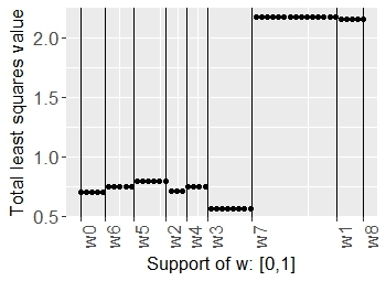
Refer to caption
Refer to caption
Figure 3: Left Panel: Step behavior of Q⁡(Nˇ,α^,τ)Q({\check{N}},\hat{\alpha},\tau) over τ∈Supp⁡(w),\tau\in{\rm Supp}(w), Q⁡(Nˇ,α^,τ)Q({\check{N}},\hat{\alpha},\tau) evaluated over grid of points τ∈{0,0.02,…,1}.\tau\in\{0,0.02,...,1\}. Here wi∼𝒰⁡(0,1),w_{i}\sim{\cal U}(0,1), n=7n=7 N=1,N=1, Nˇ=1,\check{N}=1, p=3,p=3, β(0)0=(1,0,0)T,\beta^{0}_{(0)}=(1,0,0)^{T}, β(0)0=(1,1,0)T,\beta^{0}_{(0)}=(1,1,0)^{T}, α^(0)=(0.41,0,0)T,\hat{\alpha}_{(0)}=(0.41,0,0)^{T}, α^(1)=(0.13,0.92,0)T,\hat{\alpha}_{(1)}=(0.13,0.92,0)^{T}, w0=0,w_{0}=0, w8=1.w_{8}=1. Observe that step changes occur at wiw_{i}’s. Right Panel: Construction of zero inflation for proposal density (4.4) with Nˇ=3.\check{N}=3. Zero inflation probability πi​j\pi_{ij} is controlled via a sine curve, where the period of each sine curve is different, thereby producing candidate states d,d, with all possible sparsity patterns.
 

Algorithm 4: Simulated annealing for implementation of optimization (4.2)


Let di=(d1i,…​dNˇi)d^{i}=(d_{1}^{i},...d_{\check{N}}^{i}) represent the state at the it​hi^{th} iteration, then

  • (i)

    Simulate a candidate d=(d1,…,dNˇ)Td=(d_{1},...,d_{\check{N}})^{T} from the Nˇ\check{N}-dimensional proposal density g⁡(x,di,b,πi)g(x;d^{i};b;\pi_{i}) constructed in (4.4), where πi=(πi​1,…,πi​Nˇ)T.\pi_{i}=(\pi_{i1},...,\pi_{i\check{N}})^{T}.

  • (ii)

    Accept di+1=dd^{i+1}=d with probability ρi=exp⁡(Δ​hi/Ti)∧1;\rho_{i}=\exp\big(\Delta h_{i}/T_{i}\big)\wedge 1; take di+1=did^{i+1}=d^{i} otherwise.

  • (iii)

    Update TiT_{i} to Ti+1,T_{i+1}, and πi​j\pi_{ij} to π(i+1)​j,\pi_{(i+1)j}, for each j=1,…,Nˇ.j=1,...,\check{N}.


Here Δ​hi=h⁡(di)−h⁡(d),\Delta h_{i}=h(d^{i})-h(d), where h⁡(d)=Q⁡(Nˇ,α^,τ)+μ​∑j=1Nˇ‖djn‖0.h(d)=Q(\check{N},\hat{\alpha},\tau)+\mu\sum_{j=1}^{\check{N}}\|\frac{d_{j}}{n}\|_{0}. Also, Ti,T_{i}, i=1,..,ni=1,..,n represents a user chosen decreasing sequence of positive numbers, which is also commonly referred to as the ‘temperature function’ of simulated annealing. An illustration of the evolution of the simulated annealing algorithm with the above described proposal density for the optimization (4.2) is provided in Figure 4. The following subsection provides numerical results obtained via monte carlo simulations of the methodology described here.
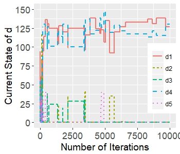
Refer to caption
Figure 4: Illustration of the evolution of simulated annealing for the optimization (4.2) to obtain d^=(d^1,…,d^Nˇ)T.\hat{d}=(\hat{d}_{1},...,\hat{d}_{\check{N}})^{T}. Here n=375,n=375, p=50,p=50, N=2,N=2, Nˇ=5,\check{N}=5, μ=0.25.\mu=0.25. The true change points are located at τ10=125\tau_{1}^{0}=125 and τ20=250.\tau_{2}^{0}=250. The proposal density is that in (4.4), with aj=1/(250+25∗(j−1)),a_{j}=1\big/\big(250+25*(j-1)\big), j=1,…,Nˇ.j=1,...,\check{N}. The temperature function is set to Ti=1/log⁡(1+i),T_{i}=1/\log(1+i), i=1,…,10000.i=1,...,10000. Observe that all but all but the components d^1,\hat{d}_{1}, d^4\hat{d}_{4} converge to zero and d^1\hat{d}_{1} converges to 127127 and d^1+d^2+d^3\hat{d}_{1}+\hat{d}_{2}+\hat{d}_{3} converges to 257,257, which are near the locations of the true change point parameters. Starting value in the algorithm: d=(94,56,56,56,56),d=(94,56,56,56,56), i.e., τ=(94,150,206,262,318).\tau=(94,150,206,262,318).
Remark 4.1.

The construction of the surrogate change inducing variable wi∗,w_{i}^{*}, the reparameterizaton of (4.1) and (4.2) is required only to avoid coding complexity of the algorithm. In general, a similar simulated annealing approach can be easily developed for directly implementing Step 1 of Algorithm 1 on the state space {−∞,w1,…,wn,∞}Nˇ,\{-\infty,w_{1},...,w_{n},\infty\}^{\check{N}}, however to avoid redundancy, these details are omitted.

4.2 Numerical Results

The main objective of the monte carlo simulations of this section are to assess the empirical performance of Algorithm 1 of the proposed method, which performs the detection and estimation of change points in the assumed model. We do not perform simulations for Algorithm 3 of the process since this step is an ordinary lasso optimization, whose empirical validity has been established in the literature via an innumerable number of simulations.

In view of the reparameterization described earlier in this section, we consider the data generating process given in (4.1). The r.v.’s εi,\varepsilon_{i}, wiw_{i} and xix_{i} are drawn independently satisfying εi∼𝒩⁡(0,σε2),\varepsilon_{i}\sim{\cal N}(0,\sigma_{\varepsilon}^{2}), and xi∼𝒩⁡(0,Σ).x_{i}\sim{\cal N}(0,\Sigma). Here, Σ\Sigma is a p×pp\times p matrix with elements Σi​j=ρ|i−j|,\Sigma_{ij}=\rho^{|i-j|}, i,j=1,…,p.i,j=1,...,p. We set, σε=1\sigma_{\varepsilon}=1 and ρ=0.5.\rho=0.5. The number of change points NN is set to one of {0,1,…,4},\{0,1,...,4\}, i.e., we consider one to five segment models. The case of N=0,N=0, where no change points are assumed is only a detection problem, as opposed to the remaining cases where the objective is both detection and estimation of change points. The change point parameters are assumed to be equally spaced in (0,1),(0,1), specifically, we set τ1†=1N+1,τ2†=2N+1,…,τN†=NN+1.\tau_{1}^{\dagger}=\frac{1}{N+1},\tau_{2}^{\dagger}=\frac{2}{N+1},...,\tau_{N}^{\dagger}=\frac{N}{N+1}. Simulations are performed for all combinations of the parameters p∈{50,175,300},p\in\{50,175,300\}, and n∈{250,375,500,625}.n\in\{250,375,500,625\}. Note that the total number of parameters to be estimated for each combination of (p,N)(p,N) is p⁡(N+1)+N.p(N+1)+N. The regression coefficients are set in the following manner. The even numbered regression coefficient vectors β2​j0=(11×5,01×(p−5))T,\beta^{0}_{2j}=(1_{1\times 5},0_{1\times(p-5)})^{T}, for all j≥0,j\geq 0, such that 2​j≤N,2j\leq N, and the odd numbered coefficient vectors are chosen as β2​j+10=(01×5,11×5,01×(p−5))T,\beta^{0}_{2j+1}=(0_{1\times 5},1_{1\times 5},0_{1\times(p-5)})^{T}, for all j≥0,j\geq 0, such that 2​j+1≤N.2j+1\leq N. Here 01×5=(0,…,0)1×5,0_{1\times 5}=(0,...,0)_{1\times 5}, 11×5=(1,…,1)1×5,1_{1\times 5}=(1,...,1)_{1\times 5}, and 01×(p−5)=(0,…,0)1×(p−5).0_{1\times(p-5)}=(0,...,0)_{1\times(p-5)}. The initial number of change points assumed in Step 0 of Algorithm 1a are set to Nˇ=4,5,6,7\check{N}=4,5,6,7 for n=250,375,500,625,n=250,375,500,625, respectively. Finally, the parameters of the simulated annealing optimization are chosen as follows. The total number of iterations performed under simulated annealing is set to M=10,000,M=10,000, the temperature function (over iterations) is set to Ti=1/(t​e​m​p∗log⁡(1+i)),T_{i}=1\big/(temp*\log(1+i)), t​e​m​p=1.25,temp=1.25, i=1,…,M.i=1,...,M. The period of sine curves constructed for zero inflation of the proposal density described in Section 4.1 is chosen as aj=1/(250+25∗(j−1)),a_{j}=1\big/\big(250+25*(j-1)\big), j=1,…,Nˇ,j=1,...,\check{N}, i.e., the first component of proposal completed 250250 oscillations within the MM iterations and each following component has 2525 more oscillations than the previous.

All results are based on 100 monte carlo repetitions. Computations are performed in the software R, R Core Team, 2017. All lasso optimizations are performed with the R package ‘glmnet’, developed by Friedman et al. , 2010. For reporting our results, we compute monte carlo approximations of the following metrics. On the detection of change points: Probability of match (PrM)=E𝟏[N~=N],{\rm(PrM)}=E{\bf 1}[\tilde{N}=N], Probability of exceeding (PrE)=E𝟏[N~>N],{\rm(PrE)}=E{\bf 1}[\tilde{N}>N], and Probability of lower number (PrL)=E𝟏[N~<N],{\rm(PrL)}=E{\bf 1}[\tilde{N}<N], Bias⁡(N~)=E⁡(N~−N),{\rm Bias}(\tilde{N})=E(\tilde{N}-N), RMSE⁡(N~)=(E​(N~−N)2)12.{\rm RMSE}(\tilde{N})=\big(E(\tilde{N}-N)^{2}\big)^{\frac{1}{2}}. On the estimation of location of change points conditioned on correct recovery of the number of change points: Bias⁡(L)=‖E⁡(τ~−τ|N~=N)‖2,{\rm Bias(L)}=\|E\big(\tilde{\tau}-\tau\big|\tilde{N}=N\big)\|_{2}, and RMSE⁡(L)=‖(E⁡((τ~−τ)2|N~=N))12‖1.{\rm RMSE(L)}=\|\big(E\big((\tilde{\tau}-\tau)^{2}\big|\tilde{N}=N\big)\big)^{\frac{1}{2}}\|_{1}.

Choice of tuning parameters λ0,λ1,μ\lambda_{0},\lambda_{1},\mu: For lasso optimization of Step 0, the regularization parameter λ0\lambda_{0} is chosen via a 5-fold cross validation (performed internally by the R package ‘glmnet’). Next, we use a BIC-type criteria to choose the regularizer μ\mu of Step 1 of Algorithm 1a. Specifically, let d^​(μ)\hat{d}(\mu) represent the solution of (4.2) and τ^​(μ)\hat{\tau}(\mu) be the corresponding change point solution, then we choose μ\mu as argument that minimizes the criteria,

BIC⁡(μ)=log⁡(Q⁡(Nˇ,α^,τ^​(μ)))+c​‖d^​(μ)‖0​log⁡nn\displaystyle{\rm BIC}(\mu)=\log\big(Q\big(\check{N},\hat{\alpha},\hat{\tau}(\mu)\big)\big)+c\frac{\|\hat{d}(\mu)\|_{0}\log n}{n} (4.5)

Here we set c=10,c=10, which performs well in all empirically examined cases.

The simulation results for p=50,175,300p=50,175,300 are reported in Table 1, Table 2 and Table 3, respectively. The results are encouraging and supportive of our theoretical findings. For nearly all examined cases, in ≈80%\approx 80\% of all simulations, the estimated number of change points match exactly with the unknown number of change points. In cases where there is mismatch between N~\tilde{N} and N,N, it can be approximated from Bias⁡(N~){\rm Bias}(\tilde{N}) and RMSE⁡(N~),{\rm RMSE}(\tilde{N}), that the proposed procedure misses the unknown number of change points by ≈1\approx 1 change point. In these cases of mismatch, it is also observed that under the given settings, N~\tilde{N} exceeds N,N, indicating the BIC selection criteria can be further tightened by increasing the value of the constant chosen in its definition. Additionally, it is also observed from Bias⁡(L),{\rm Bias(L)}, and RMSE⁡(L){\rm RMSE(L)} that the components of τ~\tilde{\tau} precisely converge toward the locations of the unknown change points, however, as expected some deterioration in accuracy is observed as pp increases.

Table 1: Numerical results on the performance of Algorithm 1 in estimating the number of change points NN and their locations τ0,\tau^{0}, when p=50.p=50.
nn NN Nˇ\check{N} PrM PrE PrL Bias(N) RMSE(N) Bias(L) RMSE(L)
250 0 4 0.82 0.18 0 0.19 0.458258 NA NA
250 1 4 0.94 0.06 0 0.06 0.244949 8.51E-05 0.007449
375 0 5 0.93 0.07 0 0.09 0.360555 NA NA
375 1 5 0.97 0.03 0 0.03 0.173205 0.000137 0.005215
375 2 5 0.95 0.05 0 0.05 0.223607 0.000465 0.013372
500 0 6 0.94 0.06 0 0.08 0.34641 NA NA
500 1 6 0.98 0.02 0 0.03 0.223607 0.000857 0.004755
500 2 6 0.92 0.08 0 0.08 0.282843 0.000724 0.01201
500 3 6 0.93 0.07 0 0.07 0.264575 0.001743 0.030009
625 0 7 0.97 0.03 0 0.04 0.244949 NA NA
625 1 7 0.94 0.06 0 0.06 0.244949 0.000749 0.004155
625 2 7 0.76 0.24 0 0.26 0.547723 0.000426 0.012903
625 3 7 0.55 0.45 0 0.51 0.806226 0.001581 0.033614
625 4 7 0.72 0.28 0 0.3 0.583095 0.003469 0.070702
Table 2: Numerical results on the performance of Algorithm 1 in estimating the number of change points NN and their locations τ0,\tau^{0}, when p=175.p=175.
nn NN Nˇ\check{N} PrM PrE PrL Bias(N) RMSE(N) Bias(L) RMSE(L)
250 0 4 0.74 0.26 0 0.28 0.565685 NA NA
250 1 4 0.93 0.07 0 0.07 0.264575 0.001462 0.006941
375 0 5 0.87 0.13 0 0.13 0.360555 NA NA
375 1 5 0.95 0.05 0 0.05 0.223607 0.00073 0.006646
375 2 5 0.97 0.03 0 0.03 0.173205 0.000505 0.013853
500 0 6 0.9 0.1 0 0.14 0.489898 NA NA
500 1 6 0.92 0.08 0 0.1 0.374166 0.000283 0.005345
500 2 6 0.92 0.08 0 0.09 0.331662 0.000997 0.014112
500 3 6 0.98 0.02 0 0.02 0.141421 0.002776 0.031699
625 0 7 0.94 0.06 0 0.08 0.34641 NA NA
625 1 7 0.96 0.04 0 0.04 0.2 1.58E-20 0.004888
625 2 7 0.73 0.27 0 0.28 0.547723 0.001232 0.015207
625 3 7 0.56 0.44 0 0.51 0.818535 0.001971 0.031628
625 4 7 0.77 0.23 0 0.23 0.479583 0.001937 0.076667
Table 3: Numerical results on the performance of Algorithm 1 in estimating the number of change points NN and their locations τ0,\tau^{0}, when p=300.p=300.
nn NN Nˇ\check{N} PrM PrE PrL Bias(N) RMSE(N) Bias(L) RMSE(L)
250 0 4 0.65 0.35 0 0.38 0.663325 NA NA
250 1 4 0.93 0.07 0 0.07 0.264575 0.000344 0.006479
375 0 5 0.81 0.19 0 0.23 0.556776 NA NA
375 1 5 0.97 0.03 0 0.03 0.173205 0.000687 0.00773
375 2 5 0.94 0.06 0 0.06 0.244949 0.00205 0.015561
500 0 6 0.87 0.13 0 0.16 0.469042 NA NA
500 1 6 0.92 0.08 0 0.09 0.331662 0.000739 0.005421
500 2 6 0.93 0.07 0 0.07 0.264575 0.000882 0.015368
500 3 6 0.95 0.05 0 0.05 0.223607 0.001901 0.033745
625 0 7 0.86 0.14 0 0.19 0.538516 NA NA
625 1 7 0.92 0.08 0 0.1 0.374166 0.000313 0.005492
625 2 7 0.82 0.18 0 0.18 0.424264 0.001554 0.015243
625 3 7 0.53 0.47 0 0.5 0.748331 0.0013 0.030562
625 4 7 0.77 0.23 0 0.25 0.538516 0.002367 0.069581

5 Discussion

Dynamic high dimensional regression models which are characterized via change points, provide an intuitive modelling approach that allows for dynamic behavior of parameters. These models allow for much greater versatility of the assumed model, and consequently a greater fidelity to the data structure. These models have been sparsely used in applications due to gaps in theoretical understanding and a lack of availability of efficient methods for estimation of parameters for such models. This article serves to fill this void. We develop a novel methodology for the detection and estimation of multiple change points in high dimensional linear regression models. The proposed method is theoretically sound and empirically more efficient than methods currently available in the literature. The idea of arbitrary segmentation is not restricted to regression models and the proposed methodology could potentially be developed for other relevant models such as dynamic networks. Two technical questions remained unanswered. First, what is optimal rate of regularized change point estimates in a high dimensional setting such as the one considered in this article. Second, is there theoretical validity of a BIC type criteria for the selection of the regularization parameter in the ℓ0\ell_{0} regularization considered in this article. However these questions are left open for further investigations.

References

  • Atchade & Bybee, (2017) Atchade, Yves, & Bybee, Leland. 2017. A scalable algorithm for gaussian graphical models with change-points. arxiv preprint arxiv:1707.04306.
  • Bai, (1997) Bai, Jushan. 1997. Estimation of a change point in multiple regression models. Review of economics and statistics, 79(4), 551–563.
  • Belloni et al. , (2011) Belloni, Alexandre, Chernozhukov, Victor, & Wang, Lie. 2011. Square-root lasso: pivotal recovery of sparse signals via conic programming. Biometrika, 98(4), 791–806.
  • Belloni et al. , (2017a) Belloni, Alexandre, Rosenbaum, Mathieu, & Tsybakov, Alexandre B. 2017a. Linear and conic programming estimators in high dimensional errors-in-variables models. Journal of the royal statistical society: Series b (statistical methodology), 79(3), 939–956.
  • Belloni et al. , (2017b) Belloni, Alexandre, Chernozhukov, Victor, Kaul, Abhishek, Rosenbaum, Mathieu, & Tsybakov, Alexandre B. 2017b. Pivotal estimation via self-normalization for high-dimensional linear models with error in variables. arxiv preprint arxiv:1708.08353.
  • Bickel et al. , (2009) Bickel, Peter J., Ritov, Ya’acov, Tsybakov, Alexandre B., et al. . 2009. Simultaneous analysis of lasso and dantzig selector. The annals of statistics, 37(4), 1705–1732.
  • Bühlmann & Van De Geer, (2011) Bühlmann, Peter, & Van De Geer, Sara. 2011. Statistics for high-dimensional data: methods, theory and applications. Springer Science & Business Media.
  • Cho & Fryzlewicz, (2015) Cho, Haeran, & Fryzlewicz, Piotr. 2015. Multiple-change-point detection for high dimensional time series via sparsified binary segmentation. Journal of the royal statistical society: Series b (statistical methodology), 77(2), 475–507.
  • Ciuperca, (2014) Ciuperca, Gabriela. 2014. Model selection by lasso methods in a change-point model. Statistical papers, 55(2), 349–374.
  • Durrett, (2010) Durrett, Rick. 2010. Probability: theory and examples. Cambridge university press.
  • Friedman et al. , (2010) Friedman, Jerome, Hastie, Trevor, & Tibshirani, Robert. 2010. glmnet: lasso and elastic-net regularized generalized linear models, 2010b. Url http://cran. r-project. org/package= glmnet. r package version, 1–1.
  • Fryzlewicz, (2014) Fryzlewicz, Piotr. 2014. Wild binary segmentation for multiple change-point detection. The annals of statistics, 42(6), 2243–2281.
  • Gautier & Tsybakov, (2011) Gautier, Eric, & Tsybakov, Alexandre. 2011. High-dimensional instrumental variables regression and confidence sets. arxiv preprint arxiv:1105.2454.
  • Gibberd & Roy, (2017) Gibberd, Alex J., & Roy, Sandipan. 2017. Multiple changepoint estimation in high-dimensional gaussian graphical models. arxiv preprint arxiv:1712.05786.
  • Hastie et al. , (2015) Hastie, Trevor, Tibshirani, Robert, & Wainwright, Martin. 2015. Statistical learning with sparsity: the lasso and generalizations. CRC press.
  • Hinkley, (1969) Hinkley, David V. 1969. Inference about the intersection in two-phase regression. Biometrika, 56(3), 495–504.
  • Hinkley, (1970) Hinkley, David V. 1970. Inference about the change-point in a sequence of random variables. Biometrika.
  • Hinkley, (1972) Hinkley, David V. 1972. Time-ordered classification. Biometrika, 59(3), 509–523.
  • Jandhyala & Fotopoulos, (1999) Jandhyala, Venkata K., & Fotopoulos, Stergios B. 1999. Capturing the distributional behaviour of the maximum likelihood estimator of a changepoint. Biometrika, 86(1), 129–140.
  • Jandhyala & MacNeill, (1997) Jandhyala, Venkata K., & MacNeill, Ian B. 1997. Iterated partial sum sequences of regression residuals and tests for changepoints with continuity constraints. Journal of the royal statistical society: Series b (statistical methodology), 59(1), 147–156.
  • Jandhyala et al. , (2013) Jandhyala, Venkata K., Fotopoulos, Stergios B., MacNeill, Ian B., & Liu, Pengyu. 2013. Inference for single and multiple change-points in time series. Journal of time series analysis, 34(4), 423–446.
  • Jin et al. , (2016) Jin, Baisuo, Wu, Yuehua, & Shi, Xiaoping. 2016. Consistent two-stage multiple change-point detection in linear models. Canadian journal of statistics, 44(2), 161–179.
  • Kaul, (2014) Kaul, Abhishek. 2014. Lasso with long memory regression errors. Journal of statistical planning and inference, 153, 11–26.
  • Kaul & Koul, (2015) Kaul, Abhishek, & Koul, Hira L. 2015. Weighted ℓ1-penalized corrected quantile regression for high dimensional measurement error models. Journal of multivariate analysis, 140, 72–91.
  • Kaul et al. , (2017) Kaul, Abhishek, Davidov, Ori, & Peddada, Shyamal D. 2017. Structural zeros in high-dimensional data with applications to microbiome studies. Biostatistics, 18(3), 422–433.
  • Kaul et al. , (2019) Kaul, Abhishek, Jandhyala, Venkata K., & Fotopoulos, Stergios B. 2019. An efficient two step algorithm for high dimensional change point regression models without grid search. Journal of machine learning research (to appear), arxiv preprint arxiv:1805.03719.
  • Koenker & Mizera, (2014) Koenker, Roger, & Mizera, Ivan. 2014. Convex optimization in r. Journal of statistical software, 60(5), 1–23.
  • Koul & Qian, (2002) Koul, Hira L., & Qian, Lianfen. 2002. Asymptotics of maximum likelihood estimator in a two-phase linear regression model. Journal of statistical planning and inference, 108(1-2), 99–119.
  • Koul et al. , (2003) Koul, Hira L., Qian, Lianfen, & Surgailis, Donatas. 2003. Asymptotics of m-estimators in two-phase linear regression models. Stochastic processes and their applications, 103(1), 123–154.
  • Lee et al. , (2016) Lee, Sokbae, Seo, Myung Hwan, & Shin, Youngki. 2016. The lasso for high dimensional regression with a possible change point. Journal of the royal statistical society: Series b (statistical methodology), 78(1), 193–210.
  • Lee et al. , (2018) Lee, Sokbae, Liao, Yuan, Seo, Myung Hwan, & Shin, Youngki. 2018. Oracle estimation of a change point in high-dimensional quantile regression. Journal of the american statistical association, 0(0), 1–11.
  • Leonardi & Bühlmann, (2016) Leonardi, Florencia, & Bühlmann, Peter. 2016. Computationally efficient change point detection for high-dimensional regression. arxiv preprint arxiv:1601.03704.
  • Loh & Wainwright, (2012) Loh, Po-Ling, & Wainwright, Martin J. 2012. High-dimensional regression with noisy and missing data: Provable guarantees with nonconvexity. Ann. statist., 40(3), 1637–1664.
  • Maurer, (2003) Maurer, Andreas. 2003. A bound on the deviation probability for sums of non-negative random variables. J. inequalities in pure and applied mathematics, 4(1), 15.
  • R Core Team, (2017) R Core Team. 2017. R: A language and environment for statistical computing. R Foundation for Statistical Computing, Vienna, Austria.
  • Raskutti et al. , (2010) Raskutti, Garvesh, Wainwright, Martin J., & Yu, Bin. 2010. Restricted eigenvalue properties for correlated gaussian designs. Journal of machine learning research, 11(Aug), 2241–2259.
  • Raskutti et al. , (2011) Raskutti, Garvesh, Wainwright, Martin J., & Yu, Bin. 2011. Minimax rates of estimation for high-dimensional linear regression over lql_{q}-balls. Ieee transactions on information theory, 57(10), 6976–6994.
  • Robert & Casella, (2013) Robert, Christian, & Casella, George. 2013. Monte carlo statistical methods. Springer Science & Business Media.
  • Roy et al. , (2017) Roy, Sandipan, Atchadé, Yves, & Michailidis, George. 2017. Change point estimation in high dimensional markov random-field models. Journal of the royal statistical society: Series b (statistical methodology), 79(4), 1187–1206.
  • Rudelson & Zhou, (2012) Rudelson, Mark, & Zhou, Shuheng. 2012. Reconstruction from anisotropic random measurements. Pages 10–1 of: Conference on learning theory.
  • Sasaki, (1987) Sasaki, Galen H. 1987. Optimization by simulated annealing: A time-complexity analysis. Tech. rept. ILLINOIS UNIV AT URBANA DEPT OF ELECTRICAL ENGINEERING.
  • Tibshirani, (1996) Tibshirani, Robert. 1996. Regression shrinkage and selection via the lasso. Journal of the royal statistical society. series b (methodological), 267–288.
  • Tibshirani, (2011) Tibshirani, Robert. 2011. Regression shrinkage and selection via the lasso: a retrospective. Journal of the royal statistical society: Series b (statistical methodology), 73(3), 273–282.
  • Vershynin, (2010) Vershynin, Roman. 2010. Introduction to the non-asymptotic analysis of random matrices. arxiv preprint arxiv:1011.3027.
  • Wang & Samworth, (2018) Wang, Tengyao, & Samworth, Richard J. 2018. High dimensional change point estimation via sparse projection. Journal of the royal statistical society: Series b (statistical methodology), 80(1), 57–83.
  • Ye & Zhang, (2010) Ye, Fei, & Zhang, Cun-Hui. 2010. Rate minimaxity of the lasso and dantzig selector for the lq loss in lr balls. Journal of machine learning research, 11(Dec), 3519–3540.
  • Zhang et al. , (2015) Zhang, Bingwen, Geng, Jun, & Lai, Lifeng. 2015. Multiple change-points estimation in linear regression models via sparse group lasso. Ieee trans. signal processing, 63(9), 2209–2224.
  • Zhao & Yu, (2006) Zhao, Peng, & Yu, Bin. 2006. On model selection consistency of lasso. Journal of machine learning research, 7(Nov), 2541–2563.
  • Zou, (2006) Zou, Hui. 2006. The adaptive lasso and its oracle properties. Journal of the american statistical association, 101(476), 1418–1429.

Supplementary Materials for “Detection and estimation of parameters in high dimensional multiple change point regression models via ℓ1/ℓ0\ell_{1}\big/\ell_{0} regularization and discrete optimization”

Appendix A Proofs of Section 3

Proof of Lemma 3.1.

We begin by proving Part (i) of this lemma. Since ℝ¯\bar{\mathbb{R}} is compact under the metric Φ⁡(⋅),\Phi(\cdot), divide the space ℝ¯\bar{\mathbb{R}} into l=1/2​unl=1/2u_{n} closed intervals (disjoint except at the boundaries), each of length 2​un.2u_{n}. Let τ1,…​τl\tau_{1},...\tau_{l} be fixed points which represent the centres of these intervals. We shall show that the following bound holds,

max⁡supτ∈ℝ¯;τ∈ℬ⁡(τj,un)j=1,…,l⁡1n​∑i=1nζi​(τ)≤cu​max⁡{log⁡pn,un},\displaystyle\max_{j=1,...,l}\sup_{\begin{subarray}{c}\tau\in\bar{\mathbb{R}};\\ \tau\in{\cal B}(\tau_{j},u_{n})\end{subarray}}\frac{1}{n}\sum_{i=1}^{n}\zeta_{i}(\tau)\leq c_{u}\max\Big\{\frac{\log p}{n},u_{n}\Big\}, (A.1)

with probability at least 1−c1​exp⁡(−c2​log⁡p),1-c_{1}\exp(-c_{2}\log p), for nn sufficiently large. Assuming (A.1), observe that any τa,τb∈ℝ¯\tau_{a},\tau_{b}\in\bar{\mathbb{R}} satisfying d⁡(τa,τb)≤un,d(\tau_{a},\tau_{b})\leq u_{n}, must lie in atmost two adjacent intervals ℬ⁡(τj,un)∪ℬ⁡(τj+1,un),{\cal B}(\tau_{j},u_{n})\cup{\cal B}(\tau_{j+1},u_{n}), for some j=1,…,l−1.j=1,...,l-1. This implies that

supτa,τb∈ℝ¯;d⁡(τa,τb)≤un1n​∑i=1nζi​(τa,τb)≤2​max⁡supτ∈ℝ¯;τ∈ℬ⁡(τj,un)j=1,…,l⁡1n​∑i=1nζi​(τ)≤cu​max⁡{log⁡pn,un},\displaystyle\sup_{\begin{subarray}{c}\tau_{a},\tau_{b}\in\bar{\mathbb{R}};\\ d(\tau_{a},\tau_{b})\leq u_{n}\end{subarray}}\frac{1}{n}\sum_{i=1}^{n}\zeta_{i}(\tau_{a},\tau_{b})\leq 2\max_{j=1,...,l}\sup_{\begin{subarray}{c}\tau\in\bar{\mathbb{R}};\\ \tau\in{\cal B}(\tau_{j},u_{n})\end{subarray}}\frac{1}{n}\sum_{i=1}^{n}\zeta_{i}(\tau)\leq c_{u}\max\Big\{\frac{\log p}{n},u_{n}\Big\},

with probability at least 1−c1​exp⁡(−c2​log⁡p).1-c_{1}\exp(-c_{2}\log p). Thus to prove part (i), it only remains to prove (A.1), this is done in the following. Consider a fixed j∈{1,…,l}j\in\{1,...,l\} and let τa>τj\tau_{a}>\tau_{j} be a boundary point on the right of τj,\tau_{j}, such that d⁡(τj,τa)=un.d(\tau_{j},\tau_{a})=u_{n}. Then note that pn:=E​ζi​(τa,τj)=d⁡(τa,τj).p_{n}:=E\zeta_{i}(\tau_{a},\tau_{j})=d(\tau_{a},\tau_{j}). Since ζi​(τa,τb),\zeta_{i}(\tau_{a},\tau_{b}), i=1,…,ni=1,...,n are Bernoulli r.v.’s, hence for any s>0,s>0, the moment generating function is given by E​exp⁡(s​ζi​(τa,τj))=qn+pn​exp⁡(s),E\exp\big(s\zeta_{i}(\tau_{a},\tau_{j})\big)=q_{n}+p_{n}\exp(s), where qn=1−pn.q_{n}=1-p_{n}. Applying the Chernoff Inequality, we obtain,

P⁡(∑i=1nζi​(τa,τj)>t+n​pn)\displaystyle P\big(\sum_{i=1}^{n}\zeta_{i}(\tau_{a},\tau_{j})>t+np_{n}\big) =\displaystyle= P⁡(e∑i=1ns​ζi​(τa,τj)>e(s​t+s​n​pn))\displaystyle P\big(e^{\sum_{i=1}^{n}s\zeta_{i}(\tau_{a},\tau_{j})}>e^{(st+snp_{n})}\big)
≤\displaystyle\leq e−s⁡(t+n​pn)​[qn+pn​es]n.\displaystyle e^{-s(t+np_{n})}[q_{n}+p_{n}e^{s}]^{n}.

Now, in order to show,

1n​∑i=1nζi​(τa,τj)≤cu​max⁡{log⁡pn,un}\displaystyle\frac{1}{n}\sum_{i=1}^{n}\zeta_{i}(\tau_{a},\tau_{j})\leq c_{u}\max\Big\{\frac{\log p}{n},u_{n}\Big\} (A.2)

with probability at least 1−c1​exp⁡(−c2​log⁡p),1-c_{1}\exp(-c_{2}\log p), we divide the argument into two cases. First, when d⁡(τa,τj)≥c​log⁡p/n,d(\tau_{a},\tau_{j})\geq c\log p/n, for some constant c>0.c>0. In this case, upon choosing t=n​d​(τa,τj)t=nd(\tau_{a},\tau_{j}) we obtain,

P⁡(∑i=1nζi​(τa,τj)>2​n​d​(τj,τa))≤e[−2​s​n​d​(τa,τj)]​[1+(d⁡(τa,τj))​(es−1)]n.\displaystyle P\big(\sum_{i=1}^{n}\zeta_{i}(\tau_{a},\tau_{j})>2nd(\tau_{j},\tau_{a})\big)\leq e^{[-2snd(\tau_{a},\tau_{j})]}[1+(d(\tau_{a},\tau_{j}))(e^{s}-1)]^{n}.

Using the deterministic inequality (1+x)k≤exp⁡(k​x),(1+x)^{k}\leq\exp(kx), for any k,x>0,k,x>0, we obtain that

P⁡(∑i=1nζi​(τa,τj)>2​n​d​(τa,τj))≤e−2​s​n​d​(τa,τj)​e(es−1)​n​d​(τa,τj)≤e−c2​log⁡p.\displaystyle P\big(\sum_{i=1}^{n}\zeta_{i}(\tau_{a},\tau_{j})>2nd(\tau_{a},\tau_{j})\big)\leq e^{-2snd(\tau_{a},\tau_{j})}e^{(e^{s}-1)nd(\tau_{a},\tau_{j})}\leq e^{-c_{2}\log p}.

The inequality to the right follows by choosing s=log⁡2,s=\log 2, which maximizes the function f⁡(s)=2​s−es+1f(s)=2s-e^{s}+1 and provides a positive value at the maximum, and by using the restriction d⁡(τa,τj)≥c​log⁡p/n.d(\tau_{a},\tau_{j})\geq c\log p/n. Next, when d(τa,τ)<clogp/n.d(\tau_{a},\tau_{)}<c\log p/n. Here choose t=c​log⁡pt=c\log p to obtain,

P⁡(∑i=1nζi​(τa,τj)>c​log⁡p+n​d​(τa,τj))\displaystyle P\big(\sum_{i=1}^{n}\zeta_{i}(\tau_{a},\tau_{j})>c\log p+nd(\tau_{a},\tau_{j})\big)\hskip 108.405pt
≤e[−s​c​log⁡p−s​n​d​(τa,τj)]​[1+(d⁡(τa,τj))​(es−1)]n.\displaystyle\leq e^{[-sc\log p-snd(\tau_{a},\tau_{j})]}[1+(d(\tau_{a},\tau_{j}))(e^{s}-1)]^{n}. (A.3)

Calling upon the inequality (1+x)k≤exp⁡(k​x),(1+x)^{k}\leq\exp(kx), for any k,x>0,k,x>0, we can bound the RHS of (A) from above by exp⁡[−s​c​log⁡p+(es−s−1)​log⁡p].\exp\big[-sc\log p+(e^{s}-s-1)\log p\big]. Now s=log⁡(1+c)s=\log(1+c) provides a positive value at the maximum, since it maximizes f⁡(s)=(1+c)​s−es+1.f(s)=(1+c)s-e^{s}+1. Then for any c>0,c>0, we obtain,

P⁡(∑i=1nζi​(τa,τj)>c​log⁡p+n​d​(τa,τj))\displaystyle P\big(\sum_{i=1}^{n}\zeta_{i}(\tau_{a},\tau_{j})>c\log p+nd(\tau_{a},\tau_{j})\big) ≤\displaystyle\leq e−c2​log⁡p.\displaystyle e^{-c_{2}\log p}.

Upon combining both cases, (A.2) follows by noting d⁡(τa,τj)=un.d(\tau_{a},\tau_{j})=u_{n}.

Now repeating the same argument for a fixed boundary point τb\tau_{b} on the left of τj,\tau_{j}, such that d⁡(τb,τj)=un,d(\tau_{b},\tau_{j})=u_{n}, and applying a union bound we obtain,

maxτ∈{τa,τb}⁡1n​∑i=1nζi​(τ,τj)≤cu​max⁡{log⁡pn,un}\displaystyle\max_{\tau\in\{\tau_{a},\tau_{b}\}}\frac{1}{n}\sum_{i=1}^{n}\zeta_{i}(\tau,\tau_{j})\leq c_{u}\max\Big\{\frac{\log p}{n},u_{n}\Big\} (A.4)

with probability at least 1−c1​exp⁡(−c2​log⁡p).1-c_{1}\exp(-c_{2}\log p). In order to show that (A.2) holds uniformly over ℬ⁡(τj,un).{\cal B}(\tau_{j},u_{n}). For this, we begin by noting that for any τ∈ℬ⁡(τj,un),\tau\in{\cal B}(\tau_{j},u_{n}), where τ>τj\tau>\tau_{j} we have ζi(τ,τj)=𝟏[wi∈(τj,τ)]≤𝟏[wi∈(τj,τa)].\zeta_{i}(\tau,\tau_{j})={\bf 1}[w_{i}\in(\tau_{j},\tau)]\leq{\bf 1}\big[w_{i}\in(\tau_{j},\tau_{a})\big]. Similarly for any τ∈𝒯⁡(τj,un)\tau\in{\cal T}(\tau_{j},u_{n}) where τ<τj\tau<\tau_{j} we have ζi(τ)≤𝟏[wi∈(τb,τj)].\zeta_{i}(\tau)\leq{\bf 1}\big[w_{i}\in(\tau_{b},\tau_{j})\big]. Thus

supτ∈ℬ⁡(τj,un)1n​∑i=1nζi​(τ,τj)≤maxτ∈{τa,τb}⁡1n​∑i=1nζi​(τ,τj)≤cu​{log⁡pn,un}.\displaystyle\hskip 28.45274pt\sup_{\tau\in{\cal B}(\tau_{j},u_{n})}\frac{1}{n}\sum_{i=1}^{n}\zeta_{i}(\tau,\tau_{j})\leq\max_{\tau\in\{\tau_{a},\tau_{b}\}}\frac{1}{n}\sum_{i=1}^{n}\zeta_{i}(\tau,\tau_{j})\leq c_{u}\Big\{\frac{\log p}{n},u_{n}\Big\}. (A.5)

with probability at least 1−c1​exp⁡(−c2​log⁡p).1-c_{1}\exp(-c_{2}\log p). Combining the bound (A.5) over all j=1,…,lj=1,...,l using a union bound, we obtain (A.1) with probability at least 1−c1​(2​un)−1​exp⁡(−c2​log⁡p).1-c_{1}(2u_{n})^{-1}\exp(-c_{2}\log p). Finally since by assumption log⁡(un−1)=O⁡(log⁡p)\log(u_{n}^{-1})=O(\log p) therefore, (A.1) holds with probability at least 1−c1​exp⁡(−c2​log⁡p),1-c_{1}\exp(-c_{2}\log p), for nn sufficiently large. This completes the proof of Part (i).

The proof of Part (ii) proceeds with a similar idea as Part (i). Divide the space ℝ¯\bar{\mathbb{R}} into l=2/vnl=2/v_{n} closed intervals (disjoint except at the boundaries), each of length vn/2.v_{n}/2. Let τ1,…​τl\tau_{1},...\tau_{l} be fixed points which represent the centres of these intervals. We shall show that,

min⁡infτ∈ℝ¯;τ∈ℬ⁡(τj,vn/4)j=1,…,l⁡1n​∑i=1nζi​(τ,τj)≥cu​vn,\displaystyle\min_{j=1,...,l}\inf_{\begin{subarray}{c}\tau\in\bar{\mathbb{R}};\\ \tau\in{\cal B}(\tau_{j},v_{n}/4)\end{subarray}}\frac{1}{n}\sum_{i=1}^{n}\zeta_{i}(\tau,\tau_{j})\geq c_{u}v_{n}, (A.6)

with probability at least 1−c1​exp⁡(−c2​log⁡p),1-c_{1}\exp(-c_{2}\log p), for nn sufficiently large. Assuming (A.6), observe that, at least one interval ℬ⁡(τj,vn/2),{\cal B}(\tau_{j},v_{n}/2), j=1,…,lj=1,...,l will be contained in the interval between any two τa,τb∈ℝ¯\tau_{a},\tau_{b}\in\bar{\mathbb{R}} satisfying d⁡(τa,τb)≥vn.d(\tau_{a},\tau_{b})\geq v_{n}. This implies that

infτa,τb∈ℝ¯;d⁡(τa,τb)≥vn1n​∑i=1nζi​(τa,τb)≥min⁡infτ∈ℝ¯;τ∈ℬ⁡(τj,vn/4)j=1,…,l⁡1n​∑i=1nζi​(τ,τj)≥cu​vn\displaystyle\inf_{\begin{subarray}{c}\tau_{a},\tau_{b}\in\bar{\mathbb{R}};\\ d(\tau_{a},\tau_{b})\geq v_{n}\end{subarray}}\frac{1}{n}\sum_{i=1}^{n}\zeta_{i}(\tau_{a},\tau_{b})\geq\min_{j=1,...,l}\inf_{\begin{subarray}{c}\tau\in\bar{\mathbb{R}};\\ \tau\in{\cal B}(\tau_{j},v_{n}/4)\end{subarray}}\frac{1}{n}\sum_{i=1}^{n}\zeta_{i}(\tau,\tau_{j})\geq c_{u}v_{n}

with probability at least 1−c1​exp⁡(−c2​log⁡p).1-c_{1}\exp(-c_{2}\log p). Thus to prove part (i), it only remains to prove (A.6). For this purpose, we use a lower bound for sums of non-negative r.v.s’ stated in Lemma B.3. This result was originally proved by Maurer, 2003. For a fixed right boundary point τa>τj\tau_{a}>\tau_{j} such that d⁡(τa,τj)=vn/4,d(\tau_{a},\tau_{j})=v_{n}/4, set t=vnt=v_{n} in Lemma B.3. Then we have

P⁡(1n​∑i=1nζi​(τa,τj)≤vn)≤exp⁡(−4​n2​vn2n​vn)≤c1​exp⁡(−c2​log⁡p),\displaystyle P\Big(\frac{1}{n}\sum_{i=1}^{n}\zeta_{i}(\tau_{a},\tau_{j})\leq v_{n}\Big)\leq\exp\Big(-4\frac{n^{2}v_{n}^{2}}{nv_{n}}\Big)\leq c_{1}\exp(-c_{2}\log p),

where the last inequality follows from vn≥c​log⁡p/n.v_{n}\geq c\log p/n. We obtain the same bound applying a similar argument for the left boundary point τb<τj\tau_{b}<\tau_{j} such that d⁡(τb,τj)=vn/4.d(\tau_{b},\tau_{j})=v_{n}/4. Now applying an elementary union bound we obtain

P⁡(minτ∈{τa,τb}⁡1n​∑i=1nζi​(τ,τj)≥cu​vn)≥1−c1​exp⁡(−c2​log⁡p).\displaystyle\hskip 14.22636ptP\Big(\min_{\tau\in\{\tau_{a},\tau_{b}\}}\frac{1}{n}\sum_{i=1}^{n}\zeta_{i}(\tau,\tau_{j})\geq c_{u}v_{n}\Big)\geq 1-c_{1}\exp(-c_{2}\log p). (A.7)

In order to obtain uniformity over τ∈{τ;d⁡(τ,τj)≥vn/4}\tau\in\big\{\tau;\,d(\tau,\tau_{j})\geq v_{n}/4\big\} note that for τ>τj,\tau>\tau_{j}, we have ζi(τ,τj)=𝟏[wi∈(τj,τ)]≥𝟏[wi∈(τj,τa]]\zeta_{i}(\tau,\tau_{j})={\bf 1}\big[w_{i}\in(\tau_{j},\tau)\big]\geq{\bf 1}[w_{i}\in(\tau_{j},\tau_{a}]] and for any τ<τj,\tau<\tau_{j}, we have ζi(τ,τj)=𝟏[wi∈(τb,τj)]≥𝟏[wi∈[τb,τj)].\zeta_{i}(\tau,\tau_{j})={\bf 1}[w_{i}\in(\tau_{b},\tau_{j})]\geq{\bf 1}[w_{i}\in[\tau_{b},\tau_{j})]. This implies that

infτ∈ℝ¯;d⁡(τ,τj)≥vn1n​∑i=1nζi​(τ,τj)≥minτ∈{τa,τb}⁡1n​∑i=1nζi​(τ,τj)≥cu​vv.\displaystyle\inf_{\begin{subarray}{c}\tau\in\bar{\mathbb{R}};\\ d(\tau,\tau_{j})\geq v_{n}\end{subarray}}\frac{1}{n}\sum_{i=1}^{n}\zeta_{i}(\tau,\tau_{j})\geq\min_{\tau\in\{\tau_{a},\tau_{b}\}}\frac{1}{n}\sum_{i=1}^{n}\zeta_{i}(\tau,\tau_{j})\geq c_{u}v_{v}. (A.8)

with probability at least 1−c1​exp⁡(−c2​log⁡p).1-c_{1}\exp(-c_{2}\log p). Finally, (A.6) follows by using a union bound over all j=1,…,Nj=1,...,N and recalling that by assumption vn≥c​log⁡p/nv_{n}\geq c\log p/n and therefore log⁡(vn−1)=O⁡(log⁡p).\log(v_{n}^{-1})=O(\log p). This complete the proof of Lemma 3.1. ∎

Proof of Lemma 3.2.

In the following let nw:=nw​(τa,τb).n^{w}:=n^{w}(\tau_{a},\tau_{b}). To prove Part (i) note that,

infτa,τb∈ℝ¯;d⁡(τa,τb)≥vninfδ∈𝔸1n​∑i∈nwδT​xi​xiT​δ=infτa,τb∈ℝ¯;d⁡(τa,τb)≥vn|nw|n​infδ∈𝔸1|nw|​∑i∈nwδT​xi​xiT​δ\displaystyle\hskip 28.45274pt\inf_{\begin{subarray}{c}\tau_{a},\tau_{b}\in\bar{\mathbb{R}};\\ d(\tau_{a},\tau_{b})\geq v_{n}\end{subarray}}\inf_{\delta\in{\mathbb{A}}}\frac{1}{n}\sum_{i\in n^{w}}\delta^{T}x_{i}x_{i}^{T}\delta=\inf_{\begin{subarray}{c}\tau_{a},\tau_{b}\in\bar{\mathbb{R}};\\ d(\tau_{a},\tau_{b})\geq v_{n}\end{subarray}}\frac{|n^{w}|}{n}\inf_{\delta\in{\mathbb{A}}}\frac{1}{|n^{w}|}\sum_{i\in n^{w}}\delta^{T}x_{i}x_{i}^{T}\delta (A.9)

Let Pw​(⋅)P_{w}(\cdot) represent the conditional probability P(⋅|w),P(\cdot|w), where w=(w1,…,wn)T.w=(w_{1},...,w_{n})^{T}. Recalling that ww is independent of x,ε,x,\varepsilon, by assumption D(iv) and applying Lemma B.5 and Lemma B.4 we obtain,

Pw​(infδ∈𝔸1|nw|​∑i∈nwδT​xi​xiT​δ≥κ​‖δ‖22−cu​cm​log⁡p|nw|​‖δ‖12)≥\displaystyle P_{w}\Big(\inf_{\delta\in{\mathbb{A}}}\frac{1}{|n^{w}|}\sum_{i\in n^{w}}\delta^{T}x_{i}x_{i}^{T}\delta\geq\kappa\|\delta\|_{2}^{2}-c_{u}c_{m}\frac{\log p}{|n^{w}|}\|\delta\|_{1}^{2}\Big)\geq\hskip 28.45274pt
1−c1​exp⁡(−c2​log⁡p)\displaystyle 1-c_{1}\exp(-c_{2}\log p) (A.10)

Since the probability in the RHS of (A) is free of w,w, taking expectations on both sides yields,

P⁡(infδ∈𝔸1|nw|​∑i∈nwδT​xi​xiT​δ≥κ​‖δ‖22−cu​cm​log⁡p|nw|​‖δ‖12)≥\displaystyle P\Big(\inf_{\delta\in{\mathbb{A}}}\frac{1}{|n^{w}|}\sum_{i\in n^{w}}\delta^{T}x_{i}x_{i}^{T}\delta\geq\kappa\|\delta\|_{2}^{2}-c_{u}c_{m}\frac{\log p}{|n^{w}|}\|\delta\|_{1}^{2}\Big)\geq\hskip 28.45274pt
1−c1​exp⁡(−c2​log⁡p)\displaystyle 1-c_{1}\exp(-c_{2}\log p) (A.11)

Recall from Part (ii) of Lemma 3.1 that infd⁡(τa,τb)≥vn|nw|/n≥cu​vn,\inf_{d(\tau_{a},\tau_{b})\geq v_{n}}|n^{w}|/n\geq c_{u}v_{n}, with probability at least 1−c1​exp⁡(−c2​log⁡p).1-c_{1}\exp(-c_{2}\log p). Also, since δ∈𝔸,\delta\in{\mathbb{A}}, hence ‖δ‖12≤cu​s​‖δ‖22.\|\delta\|_{1}^{2}\leq c_{u}s\|\delta\|_{2}^{2}. Combining these results with (A) and substituting in (A.9) we obtain,

infτa,τb∈ℝ¯;d⁡(τa,τb)≥vninfδ∈𝔸1n​∑i∈nwδT​xi​xiT​δ\displaystyle\inf_{\begin{subarray}{c}\tau_{a},\tau_{b}\in\bar{\mathbb{R}};\\ d(\tau_{a},\tau_{b})\geq v_{n}\end{subarray}}\inf_{\delta\in{\mathbb{A}}}\frac{1}{n}\sum_{i\in n^{w}}\delta^{T}x_{i}x_{i}^{T}\delta ≥\displaystyle\geq cu​cm​vn​‖δ‖22−cu​cm​s​log⁡pn​‖δ‖22\displaystyle c_{u}c_{m}v_{n}\|\delta\|_{2}^{2}-c_{u}c_{m}\frac{s\log p}{n}\|\delta\|_{2}^{2}
≥\displaystyle\geq cu​cm​vn​‖δ‖22,\displaystyle c_{u}c_{m}v_{n}\|\delta\|_{2}^{2},

with probability at least 1−c1​exp⁡(−c2​log⁡p).1-c_{1}\exp(-c_{2}\log p). Here the final inequality follows since by assumption vn≥c​s​log⁡p/n.v_{n}\geq cs\log p\big/n. This completes the proof of Part (i). The proof of Part (ii) and Part (iii) are very similar to Part (i) and thus only key steps are provided. To prove part (ii), proceed as in Part (i) to obtain,

P⁡(infδ∈𝔸21|nw|​∑i∈nwδT​xi​xiT​δ≥κ​‖δ‖22−cu​cm​log⁡p|nw|​‖δ‖12)≥\displaystyle P\Big(\inf_{\delta\in{\mathbb{A}}_{2}}\frac{1}{|n^{w}|}\sum_{i\in n^{w}}\delta^{T}x_{i}x_{i}^{T}\delta\geq\kappa\|\delta\|_{2}^{2}-c_{u}c_{m}\frac{\log p}{|n^{w}|}\|\delta\|_{1}^{2}\Big)\geq\hskip 28.45274pt
1−c1​exp⁡(−c2​log⁡p)\displaystyle 1-c_{1}\exp(-c_{2}\log p) (A.12)

In this case since δ∈𝔸2,\delta\in{\mathbb{A}}_{2}, hence ‖δ‖12≤cu​s​(‖δ‖22+ξmax2).\|\delta\|_{1}^{2}\leq c_{u}s(\|\delta\|_{2}^{2}+\xi_{\max}^{2}). Substituting this result in (A) and proceeding as in Part (i) yields,

infτa,τb∈ℝ¯;d⁡(τa,τb)≥vninfδ∈𝔸21n​∑i∈nwδT​xi​xiT​δ\displaystyle\inf_{\begin{subarray}{c}\tau_{a},\tau_{b}\in\bar{\mathbb{R}};\\ d(\tau_{a},\tau_{b})\geq v_{n}\end{subarray}}\inf_{\delta\in{\mathbb{A}}_{2}}\frac{1}{n}\sum_{i\in n^{w}}\delta^{T}x_{i}x_{i}^{T}\delta ≥\displaystyle\geq cu​cm​vn​‖δ‖22−cu​cm​s​log⁡pn​‖δ‖22−ξmax2​s​log⁡pn\displaystyle c_{u}c_{m}v_{n}\|\delta\|_{2}^{2}-c_{u}c_{m}\frac{s\log p}{n}\|\delta\|_{2}^{2}-\frac{\xi_{\max}^{2}s\log p}{n}
≥\displaystyle\geq cu​cm​vn​‖δ‖22−ξmax2​s​log⁡pn,\displaystyle c_{u}c_{m}v_{n}\|\delta\|_{2}^{2}-\frac{\xi_{\max}^{2}s\log p}{n},

with probability at least 1−c1​exp⁡(−c2​log⁡p).1-c_{1}\exp(-c_{2}\log p). This completes the proof of Part (ii). To prove Part (iii), note that

supτa,τb∈ℝ¯;d⁡(τa,τb)≤unsupδ∈𝔸1n​∑i∈nwδT​xi​xiT​δ=supτa,τb∈ℝ¯;d⁡(τa,τb)≤un|nw|n​supδ∈𝔸1|nw|​∑i∈nwδT​xi​xiT​δ\displaystyle\sup_{\begin{subarray}{c}\tau_{a},\tau_{b}\in\bar{\mathbb{R}};\\ d(\tau_{a},\tau_{b})\leq u_{n}\end{subarray}}\sup_{\delta\in{\mathbb{A}}}\frac{1}{n}\sum_{i\in n_{w}}\delta^{T}x_{i}x_{i}^{T}\delta=\sup_{\begin{subarray}{c}\tau_{a},\tau_{b}\in\bar{\mathbb{R}};\\ d(\tau_{a},\tau_{b})\leq u_{n}\end{subarray}}\frac{|n_{w}|}{n}\sup_{\delta\in{\mathbb{A}}}\frac{1}{|n_{w}|}\sum_{i\in n_{w}}\delta^{T}x_{i}x_{i}^{T}\delta

Now, from Part (i) of Lemma 3.1 we have that supd⁡(τa,τb)≤un|nw|/n≤cu​max⁡{log⁡p/n,un}.\sup_{d(\tau_{a},\tau_{b})\leq u_{n}}|n^{w}|/n\leq c_{u}\max\{\log p/n,u_{n}\}. Proceeding via the conditional probability argument described for Part (i) leads to,

supτa,τb∈ℝ¯;d⁡(τa,τb)≤unsupδ∈𝔸1n​∑i∈nwδT​xi​xiT​δ\displaystyle\sup_{\begin{subarray}{c}\tau_{a},\tau_{b}\in\bar{\mathbb{R}};\\ d(\tau_{a},\tau_{b})\leq u_{n}\end{subarray}}\sup_{\delta\in{\mathbb{A}}}\frac{1}{n}\sum_{i\in n^{w}}\delta^{T}x_{i}x_{i}^{T}\delta ≤\displaystyle\leq cu​cm​‖δ‖22​max⁡{log⁡pn,un}+cu​cm​s​log⁡pn​‖δ‖22\displaystyle c_{u}c_{m}\|\delta\|_{2}^{2}\max\Big\{\frac{\log p}{n},u_{n}\Big\}+c_{u}c_{m}\frac{s\log p}{n}\|\delta\|_{2}^{2}
≤\displaystyle\leq cu​cm​‖δ‖22​max⁡{s​log⁡pn,un}\displaystyle c_{u}c_{m}\|\delta\|_{2}^{2}\max\Big\{\frac{s\log p}{n},u_{n}\Big\}

with probability at least 1−c1​exp⁡(−c2​log⁡p).1-c_{1}\exp(-c_{2}\log p). This completes the proof of Lemma 3.2. ∎

Proof of Theorem 3.1.

First consider the case where, τa,τb∈𝒞j1.\tau_{a},\tau_{b}\in{\cal C}_{j}^{1}. Then a simple algebraic manipulation of the basic inequality 1n​Q∗​(α^,τa,τb)+λ​‖α^‖1≤1n​Q∗​(β(j−1)0,τa,τb)+λ​‖β(j−1)0‖1\frac{1}{n}Q^{*}(\hat{\alpha},\tau_{a},\tau_{b})+\lambda\|\hat{\alpha}\|_{1}\leq\frac{1}{n}Q^{*}(\beta^{0}_{(j-1)},\tau_{a},\tau_{b})+\lambda\|\beta^{0}_{(j-1)}\|_{1} yields,

1n​∑i∈nw​(τa,τb)‖xiT​(α^−β(j−1)0)‖22+λ0​‖α‖1≤\displaystyle\frac{1}{n}\sum_{i\in n^{w}(\tau_{a},\tau_{b})}\|x_{i}^{T}(\hat{\alpha}-\beta^{0}_{(j-1)})\|_{2}^{2}+\lambda_{0}\|\alpha\|_{1}\leq\hskip 36.135pt
|2n​∑i∈nw​(τa,τb)ε~i​xiT​(α^−β(j−1)0)|+λ0​‖β(j)0‖1.\displaystyle\Big|\frac{2}{n}\sum_{i\in n^{w}(\tau_{a},\tau_{b})}\tilde{\varepsilon}_{i}x_{i}^{T}(\hat{\alpha}-\beta^{0}_{(j-1)})\Big|+\lambda_{0}\|\beta^{0}_{(j)}\|_{1}. (A.13)

Here ε~i=yi−xiT​β(j−1)0.\tilde{\varepsilon}_{i}=y_{i}-x_{i}^{T}\beta^{0}_{(j-1)}. Note that ε~i\tilde{\varepsilon}_{i} may or may not be the same as εi\varepsilon_{i} depending on the index i.i. Also, we have the following bound,

1n​‖∑i∈nw​(τa,τb)ε~i​xiT‖∞\displaystyle\frac{1}{n}\Big\|\sum_{i\in n^{w}(\tau_{a},\tau_{b})}\tilde{\varepsilon}_{i}x_{i}^{T}\Big\|_{\infty}\hskip 289.07999pt
≤1n​‖∑i∈nw​(τj−10,τj0)εi​xiT‖∞+1n​‖∑i∈nw​(τa,τj−10)ε~i​xiT‖∞+1n​‖∑i∈nw​(τj0,τb)ε~i​xiT‖∞\displaystyle\leq\frac{1}{n}\Big\|\sum_{i\in n^{w}(\tau_{j-1}^{0},\tau_{j}^{0})}\varepsilon_{i}x_{i}^{T}\Big\|_{\infty}+\frac{1}{n}\Big\|\sum_{i\in n^{w}(\tau_{a},\tau_{j-1}^{0})}\tilde{\varepsilon}_{i}x_{i}^{T}\Big\|_{\infty}+\frac{1}{n}\Big\|\sum_{i\in n^{w}(\tau_{j}^{0},\tau_{b})}\tilde{\varepsilon}_{i}x_{i}^{T}\Big\|_{\infty}\hskip 28.45274pt
≤1n​‖∑i∈nw​(τj−10,τj0)εi​xiT‖∞+1n​‖∑i∈nw​(τj−10,τj0)εi​xiT‖∞+1n​‖∑i∈nw​(τj−10,τj0)εi​xiT‖∞\displaystyle\leq\frac{1}{n}\Big\|\sum_{i\in n^{w}(\tau_{j-1}^{0},\tau_{j}^{0})}\varepsilon_{i}x_{i}^{T}\Big\|_{\infty}+\frac{1}{n}\Big\|\sum_{i\in n^{w}(\tau_{j-1}^{0},\tau_{j}^{0})}\varepsilon_{i}x_{i}^{T}\Big\|_{\infty}+\frac{1}{n}\Big\|\sum_{i\in n^{w}(\tau_{j-1}^{0},\tau_{j}^{0})}\varepsilon_{i}x_{i}^{T}\Big\|_{\infty}\hskip 21.33955pt
+1n​‖∑i∈nw​(τa,τj−10)(β(j−1)0−β(j−2)0)T​xi​xiT‖∞+1n​‖∑i∈nw​(τj0,τb)(β(j)0−β(j−1)0)T​xi​xiT‖∞\displaystyle+\frac{1}{n}\Big\|\sum_{i\in n^{w}(\tau_{a},\tau_{j-1}^{0})}(\beta_{(j-1)}^{0}-\beta_{(j-2)}^{0})^{T}x_{i}x_{i}^{T}\Big\|_{\infty}+\frac{1}{n}\Big\|\sum_{i\in n^{w}(\tau_{j}^{0},\tau_{b})}(\beta_{(j)}^{0}-\beta_{(j-1)}^{0})^{T}x_{i}x_{i}^{T}\Big\|_{\infty}
≤cu​cm​log⁡pn+cu​cm​log⁡pn​max​{log⁡pn,un}+cu​cm​max​{ξmax​log⁡pn,ξmax​un}\displaystyle\leq c_{u}c_{m}\sqrt{\frac{\log p}{n}}+c_{u}c_{m}\sqrt{\frac{\log p}{n}}\max\Big\{\sqrt{\frac{\log p}{n}},\sqrt{u_{n}}\Big\}+c_{u}c_{m}\max\Big\{\frac{\xi_{\max}\log p}{n},\xi_{\max}u_{n}\Big\}
≤cu​cm​max⁡{log⁡pn,ξmax​un}=λ.\displaystyle\leq c_{u}c_{m}\max\Big\{\sqrt{\frac{\log p}{n}},\xi_{\max}u_{n}\Big\}=\lambda.\hskip 224.03743pt

The second to last inequality here follows by applying the bounds provided in Lemma B.1. Substituting the bound of the final inequality in (A), and choosing λ0=2​λ,\lambda_{0}=2\lambda, yields the relation ‖α^Sc‖1≤3​‖(α^−β(j−1)0)S‖1,\|\hat{\alpha}_{S^{c}}\|_{1}\leq 3\|(\hat{\alpha}-\beta^{0}_{(j-1)})_{S}\|_{1}, consequently the vector α^−β(j−1)0∈𝔸.\hat{\alpha}-\beta^{0}_{(j-1)}\in{\mathbb{A}}. Thus the first two inequalities of Lemma 3.2 are now applicable. From (A) and an application of Part (i) Lemma 3.2 with vn=lminv_{n}=l_{\min} we can obtain,

cu​cm​lmin​‖α^−βj−10‖22≤s​λ​‖α^−βj−10‖2,\displaystyle c_{u}c_{m}l_{\min}\|\hat{\alpha}-\beta^{0}_{j-1}\|_{2}^{2}\leq\sqrt{s}\lambda\|\hat{\alpha}-\beta^{0}_{j-1}\|_{2},

which directly implies that ‖α^−βj−10‖2≤s​λ/lmin.\|\hat{\alpha}-\beta^{0}_{j-1}\|_{2}\leq\sqrt{s}\lambda\big/l_{\min}. To obtain the ℓ1\ell_{1} bound, recall that since α^−β(j−1)0∈𝔸,\hat{\alpha}-\beta^{0}_{(j-1)}\in{\mathbb{A}}, hence ‖α^−β(j−1)0‖1≤s​‖α^−β(j−1)0‖2.\|\hat{\alpha}-\beta^{0}_{(j-1)}\|_{1}\leq\sqrt{s}\|\hat{\alpha}-\beta^{0}_{(j-1)}\|_{2}. To complete the proof of this case, note that all bounds in the above arguments hold uniformly over any τa,τb∈𝒞j1,\tau_{a},\tau_{b}\in{\cal C}^{1}_{j}, with probability at least 1−c1​exp⁡(−c2​log⁡p).1-c_{1}\exp(-c_{2}\log p). The cases of τa,τb∈𝒞j2,\tau_{a},\tau_{b}\in{\cal C}_{j}^{2}, 𝒞j3{\cal C}^{3}_{j} and 𝒞j4{\cal C}^{4}_{j} can be proved similarly. The final statement of the lemma follows by applying a union bound. ∎

Proof of Corollary 3.1.

The proof of this result is a direct consequence of Theorem 3.1. Observe that by Condition A(i) and A(ii), the initial change point vector τˇ=(τˇ1,τˇ2,…,τˇNˇ)T\check{\tau}=(\check{\tau}_{1},\check{\tau}_{2},...,\check{\tau}_{\check{N}})^{T} satisfies the following. For any j=1,…,Nj=1,...,N the pair τmj−1,τmj\tau_{m_{j}-1},\tau_{m_{j}} lies in either 𝒞j1,{\cal C}^{1}_{j}, or 𝒞j2{\cal C}^{2}_{j} as defined in Theorem 3.1. Part (i) of this corollary follows by applying Theorem 3.1. Similarly, Part (ii) follows by noting that for any j∈𝒯c,j\in{\cal T}^{c}, the pair τˇj−1,τˇj\check{\tau}_{j-1},\check{\tau}_{j} belongs to either 𝒞kj3{\cal C}_{k_{j}}^{3} or 𝒞kj4.{\cal C}_{k_{j}}^{4}. This completes the proof of this corollary. ∎

Remark A.1.

(Additional notation used in the Proof of Lemma 3.3): Recall that the set 𝒯={m0,m1,…,mN,mN+1}{\cal T}=\{m_{0},m_{1},...,m_{N},m_{N+1}\} (defined in Condition A) is the subset of indices of {0,1,2….,Nˇ+1},\{0,1,2....,\check{N}+1\}, such that the initial change point τˇmj\check{\tau}_{m_{j}} lies in a uˇ{\check{u}}-neighborhood of τj0.\tau^{0}_{j}. In the proof to follow, we use the notation ∑mj−1<l<mj,\sum_{m_{j-1}<l<m_{j}}, to represent the sum over all possible indices ll which lie between mj−1m_{j-1} and mj.m_{j}. For example, let N=2,N=2, Nˇ=5\check{N}=5 and consider any τ∈ℝ¯Nˇ\tau\in\bar{\mathbb{R}}^{\check{N}} in the orientation described in the following Figure 5.

−∞-\inftyτ10\tau_{1}^{0}τ20\tau_{2}^{0}τ1\tau_{1}τ2\tau_{2}τ3\tau_{3}τ4\tau_{4}τ5\tau_{5}∞\infty2​un\scriptstyle{2u_{n}}2​un\scriptstyle{2u_{n}}
Figure 5: A possible orientation of initializers τˇ∈ℝ5,\check{\tau}\in{\mathbb{R}}^{5}, where N=2.N=2.

Then, 𝒯={m0,m1,m2,m3}={0,3,4,6},{\cal T}=\{m_{0},m_{1},m_{2},m_{3}\}=\{0,3,4,6\}, and for j=1,j=1, we denote by,

∑mj−1<l<mjQ∗​(α(l−1),τl−1,τl)=Q∗​(α0,τ0,τ1)+Q∗​(α1,τ1,τ2)\displaystyle\sum_{m_{j-1}<l<m_{j}}Q^{*}(\alpha_{(l-1)},\tau_{l-1},\tau_{l})=Q^{*}(\alpha_{0},\tau_{0},\tau_{1})+Q^{*}(\alpha_{1},\tau_{1},\tau_{2})
Remark A.2.

(Useful observation utilized in the Proof of Lemma 3.3): Consider the following decomposition of the ℓ0\ell_{0} regularizing term in Step 1 of Algorithm 1. For any τ∈ℝNˇ\tau\in{\mathbb{R}}^{\check{N}} such that, τ∈𝒢⁡(un,vn,𝒦,𝒦2),\tau\in{\cal G}(u_{n},v_{n},{\cal K},{\cal K}_{2}), and τ∗\tau^{*} as defined in (2.5), we have that,

∑j=1Nˇ(‖d⁡(τj−1,τj)‖0−‖d⁡(τj−1∗,τj∗)‖0)=∑j∈𝒯c‖d⁡(τj−1,τj)‖0\displaystyle\sum_{j=1}^{\check{N}}\Big(\|d(\tau_{j-1},\tau_{j})\|_{0}-\|d(\tau_{j-1}^{*},\tau_{j}^{*})\|_{0}\Big)=\sum_{j\in{\cal T}^{c}}\|d(\tau_{j-1},\tau_{j})\|_{0}
+∑j=1N(∥d(τhj−1,τhj)∥0−∥d(τhj−1∗,τhj∗)∥0)\displaystyle+\sum_{j=1}^{N}\Big(\|d(\tau_{h_{j}-1},\tau_{h_{j}})\|_{0}-\|d(\tau_{h_{j}-1}^{*},\tau_{h_{j}}^{*})\|_{0}\Big)
Proof of Lemma 3.3.

Consider any τ∈𝒢⁡(un,vn,𝒦).\tau\in{\cal G}(u_{n},v_{n},{\cal K}). The proof to follow relies in part on an algebraic manipulation of 𝒰∗​(Nˇ,α^,τ){\cal U}^{*}(\check{N},\hat{\alpha},\tau) defined in (3.7), which in turn requires a decomposition of the least squares loss Q⁡(Nˇ,α,τ).Q(\check{N},\alpha,\tau). This decomposition of the least squares loss depends on the orientation of τ,\tau, and in the following we assume a specific orientation of τ,\tau, such that τhj−1≤τj0≤τhj≤τj+1,\tau_{h_{j}-1}\leq\tau^{0}_{j}\leq\tau_{h_{j}}\leq\tau_{j+1}, j=1,…,N.j=1,...,N. While assuming this orientation does lead to a loss in generality in the sense that it does not include all possible τ,\tau, however it can be observed that any orientation of τ\tau shall lead to the same lower bound, this can be verified by following the same argument as below, however with a correspondingly different decomposition of the least squares loss. We also refer to Lemma 4.1 of Kaul et al. , 2019, which provides a similar result in the special case with Nˇ=1,\check{N}=1, for further intuition as to how the same bound persists under any other orientation. In the following, for any α(j)∈ℝp,\alpha_{(j)}\in{\mathbb{R}}^{p}, j=0,…,Nˇ,j=0,...,\check{N}, let α\alpha represent the concatenation of α(j)′\alpha_{(j)}^{\prime}s. Then consider,

Q⁡(Nˇ,α,τ)\displaystyle Q(\check{N},\alpha,\tau) =\displaystyle= 1n​∑j=1Nˇ+1Q∗​(α(j−1),τj−1,τj)=1n​∑j=1N+1∑hj−1<l≤hjQ∗​(α(l−1),τl−1,τl)\displaystyle\frac{1}{n}\sum_{j=1}^{\check{N}+1}Q^{*}(\alpha_{(j-1)},\tau_{j-1},\tau_{j})=\frac{1}{n}\sum_{j=1}^{N+1}\sum_{h_{j-1}<l\leq h_{j}}Q^{*}(\alpha_{(l-1)},\tau_{l-1},\tau_{l})
=\displaystyle= 1n​∑j=1N+1∑hj−1<l<hjQ∗​(α(l−1),τl−1,τl)+1n​∑j=1N+1Q∗​(α(hj−1),τhj−1,τhj)\displaystyle\frac{1}{n}\sum_{j=1}^{N+1}\sum_{h_{j-1}<l<h_{j}}Q^{*}(\alpha_{(l-1)},\tau_{l-1},\tau_{l})+\frac{1}{n}\sum_{j=1}^{N+1}Q^{*}(\alpha_{(h_{j}-1)},\tau_{h_{j}-1},\tau_{h_{j}})
=\displaystyle= 1n​∑j=1N+1∑mj−1<l<hjQ∗​(α(l−1),τl−1,τl)+1n​∑j=1N+1Q∗​(α(hj−1),τhj−1,τj0)\displaystyle\frac{1}{n}\sum_{j=1}^{N+1}\sum_{m_{j-1}<l<h_{j}}Q^{*}(\alpha_{(l-1)},\tau_{l-1},\tau_{l})+\frac{1}{n}\sum_{j=1}^{N+1}Q^{*}(\alpha_{(h_{j}-1)},\tau_{h_{j}-1},\tau_{j}^{0})
+1n∑j=1NQ∗(α(hj−1),τj0,τhj).\displaystyle+\frac{1}{n}\sum_{j=1}^{N}Q^{*}(\alpha_{(h_{j}-1)},\tau_{j}^{0},\tau_{h_{j}}).

Now, recall the definition of τ∗\tau^{*} from (2.5) and note that,

Q⁡(Nˇ,α,τ∗)\displaystyle Q(\check{N},\alpha,\tau^{*}) =\displaystyle= 1n​∑j=1Nˇ+1Q∗​(α(j−1),τj−1∗,τj∗)=1n​∑j=1N+1Q∗​(α(hj−1),τhj−1∗,τhj∗)\displaystyle\frac{1}{n}\sum_{j=1}^{\check{N}+1}Q^{*}(\alpha_{(j-1)},\tau_{j-1}^{*},\tau_{j}^{*})=\frac{1}{n}\sum_{j=1}^{N+1}Q^{*}(\alpha_{(h_{j}-1)},\tau_{h_{j}-1}^{*},\tau_{h_{j}}^{*})
=\displaystyle= 1n​∑j=1N+1∑mj−1<l<hjQ∗​(α(hj−1),τl−1,τl)+1n​∑j=1NQ⁡(α(hj+1−1),τj0,τhj)\displaystyle\frac{1}{n}\sum_{j=1}^{N+1}\sum_{m_{j-1}<l<h_{j}}Q^{*}(\alpha_{(h_{j}-1)},\tau_{l-1},\tau_{l})+\frac{1}{n}\sum_{j=1}^{N}Q(\alpha_{(h_{j+1}-1)},\tau_{j}^{0},\tau_{h_{j}})
+1n∑j=1N+1Q∗(α(hj−1),τhj−1,τj0).\displaystyle+\frac{1}{n}\sum_{j=1}^{N+1}Q^{*}(\alpha_{(h_{j}-1)},\tau_{h_{j}-1},\tau_{j}^{0}).

Substituting the above expressions for Q⁡(Nˇ,α,τ)Q(\check{N},\alpha,\tau) and Q⁡(Nˇ,α,τ∗)Q(\check{N},\alpha,\tau^{*}) in the definition of 𝒰∗​(Nˇ,α,τ){\cal U}^{*}(\check{N},\alpha,\tau) given in (3.7), we obtain,

𝒰∗​(Nˇ,α,τ)\displaystyle{\cal U}^{*}(\check{N},\alpha,\tau) =\displaystyle= Q⁡(Nˇ,α,τ)−Q⁡(Nˇ,α,τ∗)\displaystyle Q(\check{N},\alpha,\tau)-Q(\check{N},\alpha,\tau^{*})
=\displaystyle= 1n​∑j=1N+1∑mj−1<l<hjQ∗​(α(l−1),τl−1,τl)+1n​∑j=1NQ∗​(α(hj−1),τj0,τhj)\displaystyle\frac{1}{n}\sum_{j=1}^{N+1}\sum_{m_{j-1}<l<h_{j}}Q^{*}(\alpha_{(l-1)},\tau_{l-1},\tau_{l})+\frac{1}{n}\sum_{j=1}^{N}Q^{*}(\alpha_{(h_{j}-1)},\tau_{j}^{0},\tau_{h_{j}})
−1n∑j=1NQ(α(hj+1−1),τj0,τhj)−1n∑j=1N+1∑mj−1<l<hjQ∗(α(hj−1),τl−1,τl)\displaystyle-\frac{1}{n}\sum_{j=1}^{N}Q(\alpha_{(h_{j+1}-1)},\tau_{j}^{0},\tau_{h_{j}})-\frac{1}{n}\sum_{j=1}^{N+1}\sum_{m_{j-1}<l<h_{j}}Q^{*}(\alpha_{(h_{j}-1)},\tau_{l-1},\tau_{l})
:⁣=\displaystyle:= (T​1)+(T​2)−(T​3)−(T​4)\displaystyle(T1)+(T2)-(T3)-(T4)

Further simplifying terms (T1)-(T4) we obtain,

T​1\displaystyle T1 =\displaystyle= 1n​∑j=1N+1∑mj−1<l<hjQ∗​(α(l−1),τl−1,τl)=1n​∑j=1N+1∑mj−1<l<hj∑τl−1<wi<τl(yi−xiT​α(l−1))2\displaystyle\frac{1}{n}\sum_{j=1}^{N+1}\sum_{m_{j-1}<l<h_{j}}Q^{*}(\alpha_{(l-1)},\tau_{l-1},\tau_{l})=\frac{1}{n}\sum_{j=1}^{N+1}\sum_{m_{j-1}<l<h_{j}}\sum_{\tau_{l-1}<w_{i}<\tau_{l}}\big(y_{i}-x_{i}^{T}\alpha_{(l-1)}\big)^{2}
=\displaystyle= 1n​∑j=1N+1∑mj−1<l<hj∑τl−1<wi<τlεi2−2n​∑j=1N+1∑mj−1<l<hj∑τl−1<wi<τlεi​xiT​(α(l−1)−β(j−1)0)\displaystyle\frac{1}{n}\sum_{j=1}^{N+1}\sum_{m_{j-1}<l<h_{j}}\sum_{\tau_{l-1}<w_{i}<\tau_{l}}\varepsilon_{i}^{2}-\frac{2}{n}\sum_{j=1}^{N+1}\sum_{m_{j-1}<l<h_{j}}\sum_{\tau_{l-1}<w_{i}<\tau_{l}}\varepsilon_{i}x_{i}^{T}(\alpha_{(l-1)}-\beta^{0}_{(j-1)})
+1n∑j=1N+1∑mj−1<l<hj∑τl−1<wi<τl(α(l−1)−β(j−1)0)TxixiT(α(l−1)−β(j−1)0)\displaystyle+\frac{1}{n}\sum_{j=1}^{N+1}\sum_{m_{j-1}<l<h_{j}}\sum_{\tau_{l-1}<w_{i}<\tau_{l}}(\alpha_{(l-1)}-\beta^{0}_{(j-1)})^{T}x_{i}x_{i}^{T}(\alpha_{(l-1)}-\beta^{0}_{(j-1)})
T​2\displaystyle T2 =\displaystyle= 1n​∑j=1NQ∗​(α(hj−1),τj0,τhj)=1n​∑j=1N∑i∈nw​(τj0,τhj)(yi−xiT​α(hj−1))2\displaystyle\frac{1}{n}\sum_{j=1}^{N}Q^{*}(\alpha_{(h_{j}-1)},\tau_{j}^{0},\tau_{h_{j}})=\frac{1}{n}\sum_{j=1}^{N}\sum_{i\in n^{w}(\tau^{0}_{j},\tau_{h_{j}})}\big(y_{i}-x_{i}^{T}\alpha_{(h_{j}-1)}\big)^{2}
=\displaystyle= 1n​∑j=1N∑i∈nw​(τj0,τhj)(εi−xiT​(α(hj−1)−β(j)0))2\displaystyle\frac{1}{n}\sum_{j=1}^{N}\sum_{i\in n^{w}(\tau^{0}_{j},\tau_{h_{j}})}\big(\varepsilon_{i}-x_{i}^{T}(\alpha_{(h_{j}-1)}-\beta^{0}_{(j)})\big)^{2}
=\displaystyle= 1n​∑j=1N∑i∈nw​(τj0,τhj)εi2−2n​∑j=1N∑i∈nw​(τj0,τhj)εi​xiT​(α(hj−1)−β(j)0)\displaystyle\frac{1}{n}\sum_{j=1}^{N}\sum_{i\in n^{w}(\tau^{0}_{j},\tau_{h_{j}})}\varepsilon_{i}^{2}-\frac{2}{n}\sum_{j=1}^{N}\sum_{i\in n^{w}(\tau^{0}_{j},\tau_{h_{j}})}\varepsilon_{i}x_{i}^{T}(\alpha_{(h_{j}-1)}-\beta^{0}_{(j)})
+1n∑j=1N∑i∈nw​(τj0,τhj)(α(hj−1)−β(j)0)TxixiT(α(hj−1)−β(j)0)\displaystyle+\frac{1}{n}\sum_{j=1}^{N}\sum_{i\in n^{w}(\tau^{0}_{j},\tau_{h_{j}})}(\alpha_{(h_{j}-1)}-\beta^{0}_{(j)})^{T}x_{i}x_{i}^{T}(\alpha_{(h_{j}-1)}-\beta^{0}_{(j)})
T​3\displaystyle T3 =\displaystyle= 1n​∑j=1NQ⁡(α(hj+1−1),τj0,τhj)\displaystyle\frac{1}{n}\sum_{j=1}^{N}Q(\alpha_{(h_{j+1}-1)},\tau_{j}^{0},\tau_{h_{j}})
=\displaystyle= 1n​∑j=1N∑i∈nw​(τj0,τhj)εi2−2n​∑j=1N∑i∈nw​(τj0,τhj)εi​xiT​(α(hj+1−1)−β(j)0)\displaystyle\frac{1}{n}\sum_{j=1}^{N}\sum_{i\in n^{w}(\tau^{0}_{j},\tau_{h_{j}})}\varepsilon_{i}^{2}-\frac{2}{n}\sum_{j=1}^{N}\sum_{i\in n^{w}(\tau^{0}_{j},\tau_{h_{j}})}\varepsilon_{i}x_{i}^{T}(\alpha_{(h_{j+1}-1)}-\beta^{0}_{(j)})
+1n∑j=1N∑i∈nw​(τj0,τhj)(α(hj+1−1)−β(j)0)TxixiT(α(hj+1−1)−β(j)0)\displaystyle+\frac{1}{n}\sum_{j=1}^{N}\sum_{i\in n^{w}(\tau^{0}_{j},\tau_{h_{j}})}(\alpha_{(h_{j+1}-1)}-\beta^{0}_{(j)})^{T}x_{i}x_{i}^{T}(\alpha_{(h_{j+1}-1)}-\beta^{0}_{(j)})
T​4\displaystyle T4 =\displaystyle= 1n​∑j=1N+1∑mj−1<l<hjQ∗​(α(hj−1),τl−1,τl)\displaystyle\frac{1}{n}\sum_{j=1}^{N+1}\sum_{m_{j-1}<l<h_{j}}Q^{*}(\alpha_{(h_{j}-1)},\tau_{l-1},\tau_{l})
=\displaystyle= 1n​∑j=1N+1∑mj−1<l<hj∑τl−1<wi<τl(yi−xiT​α(hj−1))2\displaystyle\frac{1}{n}\sum_{j=1}^{N+1}\sum_{m_{j-1}<l<h_{j}}\sum_{\tau_{l-1}<w_{i}<\tau_{l}}\big(y_{i}-x_{i}^{T}\alpha_{(h_{j}-1)}\big)^{2}
=\displaystyle= 1n​∑j=1N+1∑mj−1<l<hj∑τl−1<wi<τlεi2\displaystyle\frac{1}{n}\sum_{j=1}^{N+1}\sum_{m_{j-1}<l<h_{j}}\sum_{\tau_{l-1}<w_{i}<\tau_{l}}\varepsilon_{i}^{2}
−2n∑j=1N+1∑mj−1<l<hj∑τl−1<wi<τlεixiT(α(hj−1)−β(j−1)0)\displaystyle-\frac{2}{n}\sum_{j=1}^{N+1}\sum_{m_{j-1}<l<h_{j}}\sum_{\tau_{l-1}<w_{i}<\tau_{l}}\varepsilon_{i}x_{i}^{T}(\alpha_{(h_{j}-1)}-\beta^{0}_{(j-1)})
+1n∑j=1N+1∑mj−1<l<hj∑τl−1<wi<τl(α(hj−1)−β(j−1)0)TxixiT(α(hj−1)−β(j−1)0)\displaystyle+\frac{1}{n}\sum_{j=1}^{N+1}\sum_{m_{j-1}<l<h_{j}}\sum_{\tau_{l-1}<w_{i}<\tau_{l}}(\alpha_{(h_{j}-1)}-\beta^{0}_{(j-1)})^{T}x_{i}x_{i}^{T}(\alpha_{(h_{j}-1)}-\beta^{0}_{(j-1)})

Substituting the above expressions for terms (T​1)−(T​4)(T1)-(T4) back in the expression for 𝒰∗​(Nˇ,α,τ),{\cal U}^{*}(\check{N},\alpha,\tau), while also noting that all terms involving εi2\varepsilon_{i}^{2} cancel each other, we obtain,

𝒰∗​(Nˇ,α,τ)\displaystyle{\cal U}^{*}(\check{N},\alpha,\tau) =\displaystyle= 1n​∑j=1N∑i∈nw​(τj0,τhj)(α(hj−1)−β(j)0)T​xi​xiT​(α(hj−1)−β(j)0)\displaystyle\frac{1}{n}\sum_{j=1}^{N}\sum_{i\in n^{w}(\tau^{0}_{j},\tau_{h_{j}})}(\alpha_{(h_{j}-1)}-\beta^{0}_{(j)})^{T}x_{i}x_{i}^{T}(\alpha_{(h_{j}-1)}-\beta^{0}_{(j)})
+1n∑j=1N+1∑mj−1<l<hj∑τl−1<wi<τl(α(l−1)−βj−10)TxixiT(α(l−1)−β(j−1)0)\displaystyle+\frac{1}{n}\sum_{j=1}^{N+1}\sum_{m_{j-1}<l<h_{j}}\sum_{\tau_{l-1}<w_{i}<\tau_{l}}(\alpha_{(l-1)}-\beta^{0}_{j-1})^{T}x_{i}x_{i}^{T}(\alpha_{(l-1)}-\beta^{0}_{(j-1)})
−1n∑j=1N∑i∈nw​(τj0,τhj)(α(hj+1−1)−β(j)0)TxixiT(α(hj+1−1)−β(j)0)\displaystyle-\frac{1}{n}\sum_{j=1}^{N}\sum_{i\in n^{w}(\tau^{0}_{j},\tau_{h_{j}})}(\alpha_{(h_{j+1}-1)}-\beta^{0}_{(j)})^{T}x_{i}x_{i}^{T}(\alpha_{(h_{j+1}-1)}-\beta^{0}_{(j)})
−1n∑j=1N+1∑mj−1<l<hj∑τl−1<wi<τl(α(hj−1)−β(j−1)0)TxixiT(α(hj−1)−β(j−1)0)\displaystyle-\frac{1}{n}\sum_{j=1}^{N+1}\sum_{m_{j-1}<l<h_{j}}\sum_{\tau_{l-1}<w_{i}<\tau_{l}}(\alpha_{(h_{j}-1)}-\beta^{0}_{(j-1)})^{T}x_{i}x_{i}^{T}(\alpha_{(h_{j}-1)}-\beta^{0}_{(j-1)})
−2n∑j=1N+1∑mj−1<l<hj∑τl−1<wi<τlεixiT(α(l−1)−β(j−1)0)\displaystyle-\frac{2}{n}\sum_{j=1}^{N+1}\sum_{m_{j-1}<l<h_{j}}\sum_{\tau_{l-1}<w_{i}<\tau_{l}}\varepsilon_{i}x_{i}^{T}(\alpha_{(l-1)}-\beta^{0}_{(j-1)})
−2n∑j=1N∑i∈nw​(τj0,τhj)εixiT(α(hj−1)−β(j)0)\displaystyle-\frac{2}{n}\sum_{j=1}^{N}\sum_{i\in n^{w}(\tau^{0}_{j},\tau_{h_{j}})}\varepsilon_{i}x_{i}^{T}(\alpha_{(h_{j}-1)}-\beta^{0}_{(j)})
+2n∑j=1N∑i∈nw​(τj0,τhj)εixiT(α(hj+1−1)−β(j)0)\displaystyle+\frac{2}{n}\sum_{j=1}^{N}\sum_{i\in n^{w}(\tau^{0}_{j},\tau_{h_{j}})}\varepsilon_{i}x_{i}^{T}(\alpha_{(h_{j+1}-1)}-\beta^{0}_{(j)})
+2n∑j=1N+1∑mj−1<l<hj∑τl−1<wi<τlεixiT(α(hj−1)−β(j−1)0)\displaystyle+\frac{2}{n}\sum_{j=1}^{N+1}\sum_{m_{j-1}<l<h_{j}}\sum_{\tau_{l-1}<w_{i}<\tau_{l}}\varepsilon_{i}x_{i}^{T}(\alpha_{(h_{j}-1)}-\beta^{0}_{(j-1)})
:⁣=\displaystyle:= (R​1)+(R​2)−(R​3)−(R​4)−(R​5)−(R​6)+(R​7)+(R​8)\displaystyle(R1)+(R2)-(R3)-(R4)-(R5)-(R6)+(R7)+(R8)

Here, the terms (R​1),(R​3),(R​6),(R​7)(R1),(R3),(R6),(R7) are non-zero only when N≥1.N\geq 1. In the case where N=0,N=0, these four terms will be identically zero. Also note that R​2≥0,R2\geq 0, since it is a quadratic form. Observe that when 𝒰∗​(Nˇ,α,τ){\cal U}^{*}(\check{N},\alpha,\tau) is evaluated at α^,\hat{\alpha}, and at any τ∈𝒢⁡(un,vn,𝒦),\tau\in{\cal G}(u_{n},v_{n},{\cal K}), the following uniform bounds for the terms (R​1)−(R​8)(R1)-(R8) hold, each with probability at least 1−c1​N​exp⁡(−c2​log⁡p).1-c_{1}N\exp(-c_{2}\log p). These bounds for terms (R​1)−(R​8)(R1)-(R8) follow from applications of Lemma 3.2, Lemma B.1 and Corollary 3.1. Details pertaining to the derivations of these bounds are discussed in detail in Lemma B.2 in Appendix B of the supplementary materials.

R​4\displaystyle R4 =\displaystyle= 1n​∑j=1N+1∑mj−1<l<hj∑τl−1<wi<τl(α(hj−1)−β(j−1)0)T​xi​xiT​(α(hj−1)−β(j−1)0)\displaystyle\frac{1}{n}\sum_{j=1}^{N+1}\sum_{m_{j-1}<l<h_{j}}\sum_{\tau_{l-1}<w_{i}<\tau_{l}}(\alpha_{(h_{j}-1)}-\beta^{0}_{(j-1)})^{T}x_{i}x_{i}^{T}(\alpha_{(h_{j}-1)}-\beta^{0}_{(j-1)})
≤\displaystyle\leq ∑j=1N+1∑mj−1<l<hjrn2≤cu​cm​|𝒦|​rn2\displaystyle\sum_{j=1}^{N+1}\sum_{m_{j-1}<l<h_{j}}r_{n}^{2}\leq c_{u}c_{m}|{\cal K}|r_{n}^{2}
|R​5|\displaystyle|R5| ≤\displaystyle\leq 2n​∑j=1N+1∑mj−1<l<hj|∑τl−1<wi<τlεi​xiT​(α(l−1)−β(j−1)0)|\displaystyle\frac{2}{n}\sum_{j=1}^{N+1}\sum_{m_{j-1}<l<h_{j}}\Big|\sum_{\tau_{l-1}<w_{i}<\tau_{l}}\varepsilon_{i}x_{i}^{T}(\alpha_{(l-1)}-\beta^{0}_{(j-1)})\Big|
≤\displaystyle\leq 2​2n​∑j=1N+1∑mj−1<l<hjlog⁡pn​s​rn≤cu​cm​|𝒦|​s​log⁡pn​rn\displaystyle 2\frac{2}{n}\sum_{j=1}^{N+1}\sum_{m_{j-1}<l<h_{j}}\sqrt{\frac{\log p}{n}}\sqrt{s}r_{n}\leq c_{u}c_{m}|{\cal K}|\sqrt{\frac{s\log p}{n}}r_{n}
|R​8|\displaystyle|R8| ≤\displaystyle\leq 2n​∑j=1N+1∑mj−1<l<hj|∑τl−1<wi<τlεi​xiT​(α(hj−1)−β(j−1)0)|\displaystyle\frac{2}{n}\sum_{j=1}^{N+1}\sum_{m_{j-1}<l<h_{j}}\Big|\sum_{\tau_{l-1}<w_{i}<\tau_{l}}\varepsilon_{i}x_{i}^{T}(\alpha_{(h_{j}-1)}-\beta^{0}_{(j-1)})\Big|
≤\displaystyle\leq 2​∑j=1N+1∑mj−1<l<mjlog⁡pn​s​rn≤cu​cm​|𝒦|​s​log⁡pn​rn\displaystyle 2\sum_{j=1}^{N+1}\sum_{m_{j-1}<l<m_{j}}\sqrt{\frac{\log p}{n}}\sqrt{s}r_{n}\leq c_{u}c_{m}|{\cal K}|\sqrt{\frac{s\log p}{n}}r_{n}

Next, consider the following two subcases. In the first subcase, assume N=0,N=0, In this subcase R​1=R​3=R​6=R​7=0.R1=R3=R6=R7=0. Thus, combining the bounds for (R​1)−(R​8),(R1)-(R8), we obtain for this subcase,

infτ∈𝒢𝒰∗​(Nˇ,α^,τ)≥−cu​cm​|𝒦|​rn2−cu​cm​|𝒦|​s​log⁡pn​rn\displaystyle\inf_{\tau\in{\cal G}}{\cal U}^{*}(\check{N},\hat{\alpha},\tau)\geq-c_{u}c_{m}|{\cal K}|r_{n}^{2}-c_{u}c_{m}|{\cal K}|\sqrt{\frac{s\log p}{n}}r_{n}

In the second subcase, where N≥1,N\geq 1, we have,

R​1\displaystyle R1 =\displaystyle= 1n​∑j=1N∑i∈nw​(τj0,τhj)(α^(hj−1)−β(j)0)T​xi​xiT​(α^(hj−1)−β(j)0)\displaystyle\frac{1}{n}\sum_{j=1}^{N}\sum_{i\in n^{w}(\tau^{0}_{j},\tau_{h_{j}})}(\hat{\alpha}_{(h_{j}-1)}-\beta^{0}_{(j)})^{T}x_{i}x_{i}^{T}(\hat{\alpha}_{(h_{j}-1)}-\beta^{0}_{(j)})
≥\displaystyle\geq cu​cm​ξmin2​vn−cu​cm​ξmax2​s​log⁡pn\displaystyle c_{u}c_{m}\xi_{\min}^{2}v_{n}-c_{u}c_{m}\frac{\xi_{\max}^{2}s\log p}{n}
R​3\displaystyle R3 =\displaystyle= 1n​∑j=1N∑i∈nw​(τj0,τhj)(α^(hj+1−1)−β(j)0)T​xi​xiT​(α^(hj+1−1)−β(j)0)\displaystyle\frac{1}{n}\sum_{j=1}^{N}\sum_{i\in n^{w}(\tau^{0}_{j},\tau_{h_{j}})}(\hat{\alpha}_{(h_{j+1}-1)}-\beta^{0}_{(j)})^{T}x_{i}x_{i}^{T}(\hat{\alpha}_{(h_{j+1}-1)}-\beta^{0}_{(j)})
≤\displaystyle\leq cu​cm​rn2​∑j=1Nmax⁡{s​log⁡pn,un​j}\displaystyle c_{u}c_{m}r_{n}^{2}\sum_{j=1}^{N}\max\Big\{\frac{s\log p}{n},u_{nj}\Big\}
|R​6|\displaystyle|R6| ≤\displaystyle\leq 2n​∑j=1N|∑i∈nw​(τj0,τhj)εi​xiT​(α^(hj−1)−β(j)0)|\displaystyle\frac{2}{n}\sum_{j=1}^{N}\Big|\sum_{i\in n^{w}(\tau^{0}_{j},\tau_{h_{j}})}\varepsilon_{i}x_{i}^{T}(\hat{\alpha}_{(h_{j}-1)}-\beta^{0}_{(j)})\Big|
≤\displaystyle\leq cu​cm​ξmax​log⁡pn​∑j=1Nmax⁡{log⁡pn,un​j}\displaystyle c_{u}c_{m}\xi_{\max}\sqrt{\frac{\log p}{n}}\sum_{j=1}^{N}\max\Big\{\sqrt{\frac{\log p}{n}},\sqrt{u_{nj}}\Big\}
|R​7|\displaystyle|R7| ≤\displaystyle\leq 2n​∑j=1N|∑i∈nw​(τj0,τhj)εi​xiT​(α^(hj+1−1)−β(j)0)|\displaystyle\frac{2}{n}\sum_{j=1}^{N}\Big|\sum_{i\in n^{w}(\tau^{0}_{j},\tau_{h_{j}})}\varepsilon_{i}x_{i}^{T}(\hat{\alpha}_{(h_{j+1}-1)}-\beta^{0}_{(j)})\Big|
≤\displaystyle\leq cu​cm​rn​log⁡pn​∑j=1Nmax⁡{log⁡pn,un​j}.\displaystyle c_{u}c_{m}r_{n}\sqrt{\frac{\log p}{n}}\sum_{j=1}^{N}\max\Big\{\sqrt{\frac{\log p}{n}},\sqrt{u_{nj}}\Big\}.

Combining the bounds for the terms (R​1)−(R​8),(R1)-(R8), we obtain,

infτ∈𝒢𝒰∗​(Nˇ,α^,τ)≥cu​cm​ξmin2​vn−cu​cm​ξmax2​s​log⁡pn−cu​cm​rn2​∑j=1Nmax⁡{s​log⁡pn,un​j}\displaystyle\inf_{\tau\in{\cal G}}{\cal U}^{*}(\check{N},\hat{\alpha},\tau)\geq c_{u}c_{m}\xi_{\min}^{2}v_{n}-c_{u}c_{m}\frac{\xi_{\max}^{2}s\log p}{n}-c_{u}c_{m}r_{n}^{2}\sum_{j=1}^{N}\max\Big\{\frac{s\log p}{n},u_{nj}\Big\}
−cucmξmaxlog⁡pn∑j=1Nmax{log⁡pn,un​j}−cucm|𝒦|rn2\displaystyle-c_{u}c_{m}\xi_{\max}\sqrt{\frac{\log p}{n}}\sum_{j=1}^{N}\max\Big\{\sqrt{\frac{\log p}{n}},\sqrt{u_{nj}}\Big\}-c_{u}c_{m}|{\cal K}|r_{n}^{2}
−cu​cm​|𝒦|​s​log⁡pn​rn\displaystyle-c_{u}c_{m}|{\cal K}|\sqrt{\frac{s\log p}{n}}r_{n}\hskip 148.15372pt (A.14)

To complete the proof, recall the definition of 𝒰⁡(Nˇ,α^,τ){\cal U}(\check{N},\hat{\alpha},\tau) from (3.7), and observe from (A.2), that for τ∈𝒢\tau\in{\cal G}

𝒰⁡(Nˇ,α^,τ)\displaystyle{\cal U}(\check{N},\hat{\alpha},\tau) =\displaystyle= 𝒰∗​(Nˇ,α^,τ)+μ​|𝒦|\displaystyle{\cal U}^{*}(\check{N},\hat{\alpha},\tau)+\mu|{\cal K}|
+μ∑j=1N(∥d(τhj−1,τhj)∥0−∥d(τhj−1∗,τhj∗)∥0)\displaystyle+\mu\sum_{j=1}^{N}\Big(\|d(\tau_{h_{j}-1},\tau_{h_{j}})\|_{0}-\|d(\tau_{h_{j}-1}^{*},\tau_{h_{j}}^{*})\|_{0}\Big)

Now, if unu_{n} is such that it converges to zero faster than lmin,l_{\min}, i.e. un/lmin→0,u_{n}/l_{\min}\to 0, then clearly the sign of d⁡(τhj−1,τhj)d(\tau_{h_{j}-1},\tau_{h_{j}}) will be the same as that of d⁡(τhj−1∗,τhj∗),d(\tau_{h_{j}-1}^{*},\tau_{h_{j}}^{*}), for each j∈{1,…,N},j\in\{1,...,N\}, and nn sufficiently large. The statement of this lemma now follows by combining the above expression with (A) and using the assumption ξmin>cu.\xi_{\min}>c_{u}. ∎

Proof of Theorem 3.2.

To begin with, note that by Condition B(iii) we have that rn2/ξmin2=o​(s​log⁡p/n)1/k.r_{n}^{2}/\xi_{\min}^{2}=o(s\log p/n)^{1/k}. We begin by proving Part (i) of this theorem. For this purpose, first consider the case when N=0.N=0. In this in this case {h1,….,hN}=∅,\{h_{1},....,h_{N}\}=\emptyset, and thus by construction, the sequences un,u_{n}, vnv_{n} play no role in the set 𝒢⁡(𝒦):=𝒢⁡(un,vn,𝒦).{\cal G}({\cal K}):={\cal G}(u_{n},v_{n},{\cal K}). Now, applying Part (i) of Lemma 3.3, we obtain,

infτ∈𝒢𝒰⁡(Nˇ,α^,τ)≥μ|𝒦|−cu​cm​|𝒦|​rn2−cu​cm​|𝒦|​s​log⁡pn​rn,\displaystyle\inf_{\tau\in{\cal G}}{\cal U}(\check{N},\hat{\alpha},\tau)\geq\mu|{\cal K}|-c_{u}c_{m}|{\cal K}|r_{n}^{2}-c_{u}c_{m}|{\cal K}|\sqrt{\frac{s\log p}{n}}r_{n},

Now, let if possible 𝒦{\cal K} be non-empty. Then by the choice of μ=cu​cm​ρ​(s​log⁡p/n)1/k∗,\mu=c_{u}c_{m}\rho(s\log p/n)^{1/k^{*}}, where k∗=max⁡{k,2},k^{*}=\max\{k,2\}, and nn sufficiently large, we have that, infτ∈𝒢𝒰⁡(Nˇ,α^,τ)>0.\inf_{\tau\in{\cal G}}{\cal U}(\check{N},\hat{\alpha},\tau)>0. This implies that the optimizer τ^∈ℝ¯Nˇ\hat{\tau}\in\bar{\mathbb{R}}^{\check{N}} of Step 1 of Algorithm 1, cannot lie in the set 𝒢⁡(𝒦),{\cal G}({\cal K}), for any non-empty set 𝒦,{\cal K}, with probability at least 1−c1​N​exp⁡(−c2​log⁡p).1-c_{1}N\exp(-c_{2}\log p). Thus the only remaining possibility is that τ^∈ℝ¯Nˇ\hat{\tau}\in\bar{\mathbb{R}}^{\check{N}} is such that τj−1=τj,\tau_{j-1}=\tau_{j}, for all l=1,…,Nˇ,l=1,...,\check{N}, i.e., τ^j=−∞,\hat{\tau}_{j}=-\infty, j=1,…,N.j=1,...,N. This directly implies that 𝒯^​(τ^)=∅,\hat{\cal T}(\hat{\tau})=\emptyset, and consequently N~=0,\tilde{N}=0, with probability at least 1−c1​N​exp⁡(−c2​log⁡p).1-c_{1}N\exp(-c_{2}\log p). Thus proving the theorem for this case.

Next consider the case N≥1.N\geq 1. Since the optimization of Step 1 of Algorithm 1 is over a subset of τ∈ℝ¯Nˇ,\tau\in\bar{\mathbb{R}}^{\check{N}}, therefore any such τ\tau must satisfy 0≤∑j=1Nd⁡(τhj,τj0)≤un=N,0\leq\sum_{j=1}^{N}d(\tau_{h_{j}},\tau_{j}^{0})\leq u_{n}=N, consequently, τ∈𝒢:=𝒢⁡(N,0,𝒦),\tau\in{\cal G}:={\cal G}(N,0,{\cal K}), for some 𝒦⊆𝒯c.{\cal K}\subseteq{\cal T}^{c}. Let vn≥N​s​log⁡p/nv_{n}\geq Ns\log p/n be any positive sequence, then applying Part (ii) of Lemma 3.3 over the collection 𝒢⁡(N,vn,𝒦),{\cal G}(N,v_{n},{\cal K}), yields the bound,

infτ∈𝒢𝒰⁡(Nˇ,α^,τ)\displaystyle\inf_{\tau\in{\cal G}}{\cal U}(\check{N},\hat{\alpha},\tau) ≥\displaystyle\geq cu​cm​vn+μ​|𝒦|−cu​cm​N​ρ2​s​log⁡pn−cu​cm(1∨ξmin2)​|𝒦|​rn2\displaystyle c_{u}c_{m}v_{n}+\mu|{\cal K}|-c_{u}c_{m}N\frac{\rho^{2}s\log p}{n}-\frac{c_{u}c_{m}}{(1\vee\xi_{\min}^{2})}|{\cal K}|r_{n}^{2}
−N​cu​cm(1∨ξmin2)​rn2−N​cu​cm​ρ(1∨ξmin)​s​log⁡pn\displaystyle-N\frac{c_{u}c_{m}}{(1\vee\xi_{\min}^{2})}r_{n}^{2}-N\frac{c_{u}c_{m}\rho}{(1\vee\xi_{\min})}\sqrt{\frac{s\log p}{n}}
−cu​cm(1∨ξmin2)​|𝒦|​s​log⁡pn​rn−N​μ(1∨ξmin2),\displaystyle-\frac{c_{u}c_{m}}{(1\vee\xi_{\min}^{2})}|{\cal K}|\sqrt{\frac{s\log p}{n}}r_{n}-\frac{N\mu}{(1\vee\xi_{\min}^{2})},

with probability at least 1−c1​N​exp⁡(−c2​log⁡p).1-c_{1}N\exp(-c_{2}\log p). Now, if we choose vn:=vn∗=cu​cm​N​ρ​(s​log⁡p/n)1/k∗.v_{n}:=v_{n}^{*}=c_{u}c_{m}N\rho(s\log p/n)^{1/k^{*}}. Then for nn sufficiently large we have, infτ∈𝒢𝒰∗​(Nˇ,α^,τ)>0.\inf_{\tau\in{\cal G}}{\cal U}^{*}(\check{N},\hat{\alpha},\tau)>0. This implies that the optimizer τ^\hat{\tau} cannot lie in the set 𝒢⁡(N,vn∗,𝒦),{\cal G}(N,v_{n}^{*},{\cal K}), and thus τ^∈𝒢⁡(vn∗,0,𝒦),\hat{\tau}\in{\cal G}(v_{n}^{*},0,{\cal K}), for some 𝒦.{\cal K}. This statement together with Condition C(ii) also implies that all τ^hj\hat{\tau}_{h_{j}}’s are finite and distinct, thereby implying that N~≥N.\tilde{N}\geq N. Now, for any non empty 𝒦,{\cal K}, reset un=vn∗u_{n}=v_{n}^{*} and apply Part (ii) of Lemma 3.3 over the collection 𝒢⁡(un,0,𝒦).{\cal G}(u_{n},0,{\cal K}). Noting that in this case F⁡(un)=0,F(u_{n})=0, we obtain,

infτ∈𝒢𝒰⁡(Nˇ,α^,τ)\displaystyle\inf_{\tau\in{\cal G}}{\cal U}(\check{N},\hat{\alpha},\tau) ≥\displaystyle\geq μ​|𝒦|−cu​cm​N​ρ2​s​log⁡pn−cu​cm(1∨ξmin2)​|𝒦|​rn2\displaystyle\mu|{\cal K}|-c_{u}c_{m}N\frac{\rho^{2}s\log p}{n}-\frac{c_{u}c_{m}}{(1\vee\xi_{\min}^{2})}|{\cal K}|r_{n}^{2}
−cu​cm(1∨ξmin2)​rn2​un−cu​cm​ρ(1∨ξmin)​s​log⁡pn​N​un\displaystyle-\frac{c_{u}c_{m}}{(1\vee\xi_{\min}^{2})}r_{n}^{2}u_{n}-\frac{c_{u}c_{m}\rho}{(1\vee\xi_{\min})}\sqrt{\frac{s\log p}{n}}\sqrt{Nu_{n}}
−cu​cm(1∨ξmin2)​|𝒦|​s​log⁡pn​rn,\displaystyle-\frac{c_{u}c_{m}}{(1\vee\xi_{\min}^{2})}|{\cal K}|\sqrt{\frac{s\log p}{n}}r_{n},

Under the choice μ=cu​cm​ρ​(s​log⁡p/n)1/k∗,\mu=c_{u}c_{m}\rho(s\log p/n)^{1/k^{*}}, we obtain that infτ∈𝒢𝒰∗​(Nˇ,α^,τ)>0,\inf_{\tau\in{\cal G}}{\cal U}^{*}(\check{N},\hat{\alpha},\tau)>0, for any non-empty set 𝒦.{\cal K}. Consequently implying that τ^∈𝒢⁡(un,0,∅).\hat{\tau}\in{\cal G}(u_{n},0,\emptyset). In other words, there are no finite and distinct interruptions between τ^hj\hat{\tau}_{h_{j}}’s, consequently N~=N,\tilde{N}=N, with probability at least 1−c1​N​exp⁡(−c2​log⁡p).1-c_{1}N\exp(-c_{2}\log p). This proves Part (i) of this theorem.

The proof of part (ii) relies on applying the above argument to recursively tighten the bound for τ^.\hat{\tau}. We have already shown that τ^∈𝒢⁡(un,0,∅).\hat{\tau}\in{\cal G}(u_{n},0,\emptyset). Applying the same lower bound over the collection 𝒢⁡(un,vn,∅){\cal G}(u_{n},v_{n},\emptyset) we obtain,

infτ∈𝒢𝒰⁡(Nˇ,α^,τ)\displaystyle\inf_{\tau\in{\cal G}}{\cal U}(\check{N},\hat{\alpha},\tau) ≥\displaystyle\geq cu​cm​vn−cu​cm​N​ρ2​s​log⁡pn−cu​cm(1∨ξmin2)​rn2​un\displaystyle c_{u}c_{m}v_{n}-c_{u}c_{m}N\frac{\rho^{2}s\log p}{n}-\frac{c_{u}c_{m}}{(1\vee\xi_{\min}^{2})}r_{n}^{2}u_{n}
−cu​cm​ρ(1∨ξmin)​s​log⁡pn​N​un\displaystyle-\frac{c_{u}c_{m}\rho}{(1\vee\xi_{\min})}\sqrt{\frac{s\log p}{n}}\sqrt{Nu_{n}}

Now, upon choosing,

vn≥vn∗:=cu​cm​N​ρ1+12​(s​log⁡pn)a2,with​a2=min⁡{12+12​k∗,1k∗+1k∗}\displaystyle v_{n}\geq v_{n}^{*}:=c_{u}c_{m}N\rho^{1+\frac{1}{2}}\Big(\frac{s\log p}{n}\Big)^{a_{2}},\,\,\,{\rm with}\,\,a_{2}=\min\big\{\frac{1}{2}+\frac{1}{2k^{*}},\frac{1}{k^{*}}+\frac{1}{k^{*}}\big\}

with, we obtain that for nn large, infτ∈𝒢𝒰∗​(Nˇ,α^,τ)>0.\inf_{\tau\in{\cal G}}{\cal U}^{*}(\check{N},\hat{\alpha},\tau)>0. Thus implying that τ^∈𝒢⁡(vn∗,0,∅),\hat{\tau}\in{\cal G}(v_{n}^{*},0,\emptyset), i.e., ∑j=1Nd⁡(τ^hj,τj0)≤vn∗,\sum_{j=1}^{N}d(\hat{\tau}_{h_{j}},\tau^{0}_{j})\leq v_{n}^{*}, with probability at least 1−c1​N​exp⁡(−c2​log⁡p).1-c_{1}N\exp(-c_{2}\log p). Note that, by using the above recursive argument we have tightened the desired rate at each step. Continuing these recursions, by resetting unu_{n} to the bound of the previous recursion, and applying Part (ii) of Lemma 3.3 over the collection 𝒢⁡(un,vn,∅),{\cal G}(u_{n},v_{n},\emptyset), we can obtain for the mt​hm^{th} recursion that,

∑j=1Nd⁡(τ^hj,τj0)≤cu​cm​ρbm​(s​log⁡pn)am,where,\displaystyle\sum_{j=1}^{N}d(\hat{\tau}_{h_{j}},\tau^{0}_{j})\leq c_{u}c_{m}\rho^{b_{m}}\Big(\frac{s\log p}{n}\Big)^{a_{m}},\quad{\rm where,}
am=min⁡{12+am−12,1k∗+am−1},and​bm=1+bm−12,\displaystyle a_{m}=\min\Big\{\frac{1}{2}+\frac{a_{m-1}}{2},\,\frac{1}{k^{*}}+a_{m-1}\Big\},\,\,{\rm and}\,\,b_{m}=1+\frac{b_{m-1}}{2}\hskip-28.45274pt,

additionally a1=1/k∗a_{1}=1/k^{*} and b1=1.b_{1}=1. To finish the proof, note that if we continue the above recursions an infinite number of times, we obtain a∞=∑m=1∞1/2m=1a_{\infty}=\sum_{m=1}^{\infty}1/2^{m}=1 and b∞=1+∑m=1∞1/2m=2.b_{\infty}=1+\sum_{m=1}^{\infty}1/2^{m}=2. Note that, despite the recursions in the above argument, the probability of the bound obtained after every recursion is maintained to be at least 1−c1​N​exp⁡(−c2​log⁡p),1-c_{1}N\exp(-c_{2}\log p), this follows from Remark A.3. This completes the proof of this theorem. ∎

Remark A.3.

(Observation utilized in the proof of Theorem 3.2): The proof of Theorem 3.2 relies on recursive application of Lemma 3.3. This in turn requires recursive application of the bounds of Lemma B.2, the probability of all bounds holding simultaneously at each recursion being at least 1−c1​N​exp⁡(−c2​log⁡p).1-c_{1}N\exp(-c_{2}\log p). Despite these recursions (potentially infinite) the result from the final recursion continues to hold with probability at least 1−c1​N​exp⁡(−c2​log⁡p).1-c_{1}N\exp(-c_{2}\log p). To see this, let un→0u_{n}\to 0 be any positive sequence and let {aj}→a∞,\{a_{j}\}\to a_{\infty}, j→∞,j\to\infty, 0<aj≤1,0<a_{j}\leq 1, be any strictly increasing sequence over j=1,2,….j=1,2,.... . Then define sequences unj=unaj,u^{j}_{n}=u_{n}^{a_{j}}, j=1,2​…j=1,2... . Here note that unj+1=o⁡(unj),u_{n}^{j+1}=o(u_{n}^{j}), j=1,…,j=1,..., i.e., each sequence converges to zero faster than the preceding one. Let ℰu1,ℰu2​…{\cal E}_{u^{1}},{\cal E}_{u^{2}}... be events, each with probability 1−c1​N​exp⁡(−c2​log⁡p),1-c_{1}N\exp(-c_{2}\log p), on which the upper bounds of Lemma 3.3 hold for each un1,un2,…u^{1}_{n},u^{2}_{n},... respectively. Clearly, on the intersection of events ℰu1∩ℰu2∩….,{\cal E}_{u^{1}}\cap{\cal E}_{u^{2}}\cap...., all upper bounds of Lemma B.2 hold simultaneously over any sequence unj,u_{n}^{j}, j=1,…,∞j=1,...,\infty Now, note that by the construction of these sequences, and that these are all upper bounds, the following containment holds ℰu1⊇ℰu2⊇…⊇ℰu∞.{\cal E}_{u^{1}}\supseteq{\cal E}_{u^{2}}\supseteq...\supseteq{\cal E}_{u^{\infty}}. This implies that on the event ℰu∞{\cal E}_{u^{\infty}} all bounds of Lemma B.2 hold simultaneously for any sequence {unj},\{u_{n}^{j}\}, j=1,…,∞.j=1,...,\infty. Here ℰu∞{\cal E}_{u^{\infty}} represents the set corresponding to the sequence un∞=una∞.u_{n}^{\infty}=u_{n}^{a_{\infty}}. Also, by a single application of Lemma B.2, P⁡(ℰu∞)≥1−c1​exp⁡(−c2​log⁡p).P({\cal E}_{u^{\infty}})\geq 1-c_{1}\exp(-c_{2}\log p). The same argument can be made for the lower bound of Lemma B.2, with the direction of the containment switched.

Proof of Corollary 3.2.

First, note that from the result of Theorem 3.2, we have that N~=N\tilde{N}=N and ∑j=1Nd⁡(τ~j,τj0)≤N​ρ2​s​log⁡p/n,\sum_{j=1}^{N}d(\tilde{\tau}_{j},\tau^{0}_{j})\leq N\rho^{2}s\log p\big/n, with probability at least 1−c1​N​exp⁡(−c2​log⁡p),1-c_{1}N\exp(-c_{2}\log p), for nn sufficiently large. All arguments to follow are restricted to the event where these two results hold. Now by construction of Algorithm 2, the regression estimates α~(j),\tilde{\alpha}_{(j)}, j=0,…,Nj=0,...,N are computed based on the partition yielded by the change point estimate τ~.\tilde{\tau}. Let un​j:=|τ~j−τj0|∨|τ~j+1−τj+10|u_{nj}:=|\tilde{\tau}_{j}-\tau^{0}_{j}|\vee|\tilde{\tau}_{j+1}-\tau^{0}_{j+1}| Then, choosing λ1​j=cu​cm​max⁡{log⁡p/n,ξmax​un​j},\lambda_{1j}=c_{u}c_{m}\max\{\sqrt{\log p/n},\,\xi_{\max}u_{nj}\}, and applying Theorem 3.1, we obtain for each j=0,…,N,j=0,...,N, that,

‖α~(j)−β(j)0‖≤cu​cm​s1q​max⁡{log⁡pn,ξmax​un​j}/lmin,\displaystyle\|\tilde{\alpha}_{(j)}-\beta_{(j)}^{0}\|\leq c_{u}c_{m}s^{\frac{1}{q}}\max\Big\{\sqrt{\frac{\log p}{n}},\,\xi_{\max}u_{nj}\Big\}\Big/l_{\min}, (A.15)

with probability at least 1−c1​exp⁡(−c2​log⁡p).1-c_{1}\exp(-c_{2}\log p). Again, by Theorem 3.2 we have that ∑j=1nun​j≤cu​cm​N​ρ2​s​log⁡p/n,\sum_{j=1}^{n}u_{nj}\leq c_{u}c_{m}N\rho^{2}s\log p/n, with probability at least 1−c1​(1∨N)​exp⁡(−c2​log⁡p).1-c_{1}(1\vee N)\exp(-c_{2}\log p). Thus, summing up the bounds in (A.15) over j=0,…,Nj=0,...,N we obtain the statement of the Corollary. ∎

Appendix B Auxiliary results

Lemma B.1.

Suppose Condition D and let unu_{n} be any non-negative sequence satisfying log⁡(un−1)=O⁡(log⁡p).\log(u_{n}^{-1})=O(\log p). Then we have for any fixed δ∈ℝp\delta\in{\mathbb{R}}^{p} that,

(i)\displaystyle(i) supτa,τb∈ℝ¯;d⁡(τa,τb)≤un‖1n​∑i∈nw​(τa,τb)δT​xi​xiT‖∞≤cu​cm​‖δ‖2​max⁡{log⁡pn,un},\displaystyle\sup_{\begin{subarray}{c}\tau_{a},\tau_{b}\in\bar{\mathbb{R}};\\ d(\tau_{a},\tau_{b})\leq u_{n}\end{subarray}}\Big\|\frac{1}{n}\sum_{i\in n^{w}(\tau_{a},\tau_{b})}\delta^{T}x_{i}x_{i}^{T}\Big\|_{\infty}\leq c_{u}c_{m}\|\delta\|_{2}\max\Big\{\frac{\log p}{n},u_{n}\Big\},
(i​i)\displaystyle(ii) supτa,τb∈ℝ¯;d⁡(τa,τb)≤un1n​∑i∈nw​(τa,τb)δT​xi​xiT​δ≤cu​cm​‖δ‖22​max⁡{log⁡pn,un},\displaystyle\sup_{\begin{subarray}{c}\tau_{a},\tau_{b}\in\bar{\mathbb{R}};\\ d(\tau_{a},\tau_{b})\leq u_{n}\end{subarray}}\frac{1}{n}\sum_{i\in n^{w}(\tau_{a},\tau_{b})}\delta^{T}x_{i}x_{i}^{T}\delta\leq c_{u}c_{m}\|\delta\|_{2}^{2}\max\Big\{\frac{\log p}{n},u_{n}\Big\},
(i​i​i)\displaystyle(iii) supτa,τb∈ℝ¯;d⁡(τa,τb)≤un1n​‖∑i∈nw​(τa,τb)εi​xiT‖∞≤cu​cm​log⁡pn​max⁡{log⁡pn,un},\displaystyle\sup_{\begin{subarray}{c}\tau_{a},\tau_{b}\in\bar{\mathbb{R}};\\ d(\tau_{a},\tau_{b})\leq u_{n}\end{subarray}}\frac{1}{n}\big\|\sum_{i\in n^{w}(\tau_{a},\tau_{b})}\varepsilon_{i}x_{i}^{T}\big\|_{\infty}\leq c_{u}c_{m}\sqrt{\frac{\log p}{n}}\max\Big\{\sqrt{\frac{\log p}{n}},\sqrt{u_{n}}\Big\},

with probability at least 1−c1​exp⁡(−c2​log⁡p).1-c_{1}\exp(-c_{2}\log p).

Proof of Lemma B.1.

We begin with the proof of Part (i). Note that the RHS of the inequality in Part (i) is normalized by the ℓ2\ell_{2} norm of δ.\delta. Hence, without loss of generality we can assume ‖δ‖2=1.\|\delta\|_{2}=1. In following denote nw=nw​(τa,τb).n^{w}=n^{w}(\tau_{a},\tau_{b}). Note that if |nw|=0|n^{w}|=0 then Lemma B.1 holds trivially with probability 1,1, thus without loss of generality we shall assume that |nw|>0.|n_{w}|>0. Now, for any fixed τa,τb∈ℝ¯,\tau_{a},\tau_{b}\in\bar{\mathbb{R}}, we have

‖1n​∑i∈nwδT​xi​xiT‖∞≤|nw|n​‖1|nw|​∑i∈nwδT​xi​xiT‖∞\displaystyle\Big\|\frac{1}{n}\sum_{i\in n_{w}}\delta^{T}x_{i}x_{i}^{T}\Big\|_{\infty}\leq\frac{|n_{w}|}{n}\Big\|\frac{1}{|n_{w}|}\sum_{i\in n_{w}}\delta^{T}x_{i}x_{i}^{T}\Big\|_{\infty} (B.1)

Under Condition D(iv) and by properties of conditional expectations (see e.g. Lemma B.5), the conditional probability Pw(⋅)=P(⋅|w)P_{w}(\cdotp)=P(\cdotp|w) can be bounded by treating ww as a constant. Thus,

Pw​(‖∑i∈nwδT​xi​xiT|nw|−δT​Σ‖∞>t)≤6​p​exp⁡(−cu​|nw|​min⁡{t2σx4,tσx2})\displaystyle P_{w}\Big(\Big\|\frac{\sum_{i\in n_{w}}\delta^{T}x_{i}x_{i}^{T}}{|n_{w}|}-\delta^{T}\Sigma\Big\|_{\infty}>t\Big)\leq 6p\exp(-c_{u}|n_{w}|\min\big\{\frac{t^{2}}{\sigma_{x}^{4}},\frac{t}{\sigma_{x}^{2}}\big\})

where the above probability bound is obtained by an application of Part (ii) of Lemma 14 of Loh and Wainwright (2012): supplementary materials. This lemma is reproduced as Lemma B.6 in this section. Now choosing t=cu​max⁡{σx2​log⁡p|nw|,σx​log⁡p|nw|}t=c_{u}\max\Big\{\sigma_{x}^{2}\sqrt{\frac{\log p}{|n_{w}|}},\sigma_{x}\frac{\log p}{|n_{w}|}\Big\} we obtain,

Pw​(‖∑i∈nwδT​xi​xiT|nw|‖∞≤‖δT​Σ‖∞+cu​max⁡{σx2​log⁡p|nw|,σx​log⁡p|nw|})\displaystyle P_{w}\left(\Big\|\frac{\sum_{i\in n_{w}}\delta^{T}x_{i}x_{i}^{T}}{|n_{w}|}\Big\|_{\infty}\leq\|\delta^{T}\Sigma\|_{\infty}+c_{u}\max\Big\{\sigma_{x}^{2}\sqrt{\frac{\log p}{|n_{w}|}},\sigma_{x}\frac{\log p}{|n_{w}|}\Big\}\right)
≥1−c1​exp⁡(−c2​log⁡p).\displaystyle\geq 1-c_{1}\exp(-c_{2}\log p). (B.2)

The result in (B) together with (B.1) yields,

Pw​(‖1n​∑i∈nwδT​xi​xiT‖∞≤|nw|n​‖δT​Σ‖∞+|nw|n​cu​max⁡{σx2​log⁡p|nw|,σx​log⁡p|nw|})\displaystyle P_{w}\left(\Big\|\frac{1}{n}\sum_{i\in n_{w}}\delta^{T}x_{i}x_{i}^{T}\Big\|_{\infty}\leq\frac{|n_{w}|}{n}\|\delta^{T}\Sigma\|_{\infty}+\frac{|n_{w}|}{n}c_{u}\max\Big\{\sigma_{x}^{2}\sqrt{\frac{\log p}{|n_{w}|}},\sigma_{x}\frac{\log p}{|n_{w}|}\Big\}\right)
≥1−c1​exp⁡(−c2​log⁡p).\displaystyle\geq 1-c_{1}\exp(-c_{2}\log p).

Taking expectations on both sides and observing that the RHS of the above conditional probability is free of w,w, we obtain,

P⁡(‖1n​∑i∈nwδT​xi​xiT‖∞≤|nw|n​‖δT​Σ‖∞+|nw|n​cu​max⁡{σx2​log⁡p|nw|,σx​log⁡p|nw|})\displaystyle P\left(\Big\|\frac{1}{n}\sum_{i\in n_{w}}\delta^{T}x_{i}x_{i}^{T}\Big\|_{\infty}\leq\frac{|n_{w}|}{n}\|\delta^{T}\Sigma\|_{\infty}+\frac{|n_{w}|}{n}c_{u}\max\Big\{\sigma_{x}^{2}\sqrt{\frac{\log p}{|n_{w}|}},\sigma_{x}\frac{\log p}{|n_{w}|}\Big\}\right)\hskip-28.45274pt
≥1−c1​exp⁡(−c2​log⁡p)\displaystyle\geq 1-c_{1}\exp(-c_{2}\log p) (B.3)

On the other hand, we have by Part (i) of Lemma 3.1, that with probability at least 1−c1​exp⁡(−c2​log⁡p)1-c_{1}\exp(-c_{2}\log p) that supd⁡(τa,τb)≤un|nw|/n≤cu​max⁡{log⁡p/n,un}.\sup_{d(\tau_{a},\tau_{b})\leq u_{n}}|n_{w}|/n\leq c_{u}\max\{\log p/n,u_{n}\}. Also, it is straightforward to see that ‖δT​Σ‖∞≤cu​ϕ,\|\delta^{T}\Sigma\|_{\infty}\leq c_{u}\phi, for some constant cu>0.c_{u}>0. Thus with the same probability we have the bound,

supτ∈𝒯⁡(τ0​n,un)|nw|n​‖δT​Σ‖∞≤cu​ϕ​max⁡{ca​log⁡pn,un}.\displaystyle\sup_{\tau\in{\cal T}(\tau_{0n},u_{n})}\frac{|n_{w}|}{n}\|\delta^{T}\Sigma\|_{\infty}\leq c_{u}\phi\max\Big\{c_{a}\frac{\log p}{n},u_{n}\Big\}. (B.4)

Again applying Part (i) of Lemma 3.1 we also have the following bound with probability at least 1−c1​exp⁡(−c2​log⁡p),1-c_{1}\exp(-c_{2}\log p),

supτa,τb∈ℝ¯;d⁡(τa,τb)≤un|nw|n​log⁡p|nw|\displaystyle\sup_{\begin{subarray}{c}\tau_{a},\tau_{b}\in\bar{\mathbb{R}};\\ d(\tau_{a},\tau_{b})\leq u_{n}\end{subarray}}\frac{|n_{w}|}{n}\sqrt{\frac{\log p}{|n_{w}|}} ≤\displaystyle\leq cu​log⁡pn​max⁡{log⁡pn,un}\displaystyle c_{u}\sqrt{\frac{\log p}{n}}\max\Big\{\sqrt{\frac{\log p}{n}},\sqrt{u_{n}}\Big\} (B.5)
≤\displaystyle\leq cu​max⁡{log⁡pn,un}.\displaystyle c_{u}\max\Big\{\frac{\log p}{n},u_{n}\Big\}.

The final inequality follows upon noting that if log⁡p/n​un≥un\sqrt{\log p/n}\sqrt{u_{n}}\geq u_{n} then un≤log⁡p/n.u_{n}\leq\log p/n. Finally also note that supd⁡(τa,τb)≤un(|nw|/n)​(log⁡p/|nw|)≤log⁡p/n.\sup_{d(\tau_{a},\tau_{b})\leq u_{n}}(|n_{w}|/n)(\log p/|n_{w}|)\leq\log p/n. Part (i) of the lemma follows by combining these results together with the bounds (B.4) and (B.5) in (B). The proofs of Part (ii) and Part (iii) are similar and are thus omitted. ∎

Lemma B.2.

(Bounds used in the proof of Lemma 3.3): Let α^(j),\hat{\alpha}_{(j)}, j=0,…,Nˇj=0,...,\check{N} be the regression estimates obtained from Step 1 of Algorithm 1, 𝒯{\cal T} and 𝒯∗{\cal T}^{*} be as defined in Condition A and (2.4) respectively and let 𝒢:=𝒢⁡(un,vn,𝒦){\cal G}:={\cal G}(u_{n},v_{n},{\cal K}) be as defined in (3.8). Then assuming the conditions of Lemma 3.3, the following bounds hold with probability at least 1−c1​(1∨N)​exp⁡(−c2​log⁡p),1-c_{1}(1\vee N)\exp(-c_{2}\log p), for nn sufficiently large.

(i)\displaystyle(i) infτ∈𝒢1n​ξmin2​∑j=1N∑i∈nw​(τhj,τj0)(α^(hj−1)−β(j)0)T​xi​xiT​(α^(hj−1)−β(j)0)≥\displaystyle\inf_{\tau\in{\cal G}}\frac{1}{n\xi_{\min}^{2}}\sum_{j=1}^{N}\sum_{i\in n^{w}(\tau_{h_{j}},\tau_{j}^{0})}(\hat{\alpha}_{(h_{j}-1)}-\beta^{0}_{(j)})^{T}x_{i}x_{i}^{T}(\hat{\alpha}_{(h_{j}-1)}-\beta^{0}_{(j)})\geq
cu​cm​vn−cu​cm​N​ρ2​s​log⁡pn,\displaystyle\hskip 231.26378ptc_{u}c_{m}v_{n}-c_{u}c_{m}N\frac{\rho^{2}s\log p}{n},
(i​i)\displaystyle(ii) infτ∈𝒢1n​∑j=1N+1∑mj−1<l<hj∑τl−1<wi<τl(α^(l−1)−β(j−1)0)T​xi​xiT​(α^(l−1)−β(j−1)0)≥0,\displaystyle\inf_{\tau\in{\cal G}}\frac{1}{n}\sum_{j=1}^{N+1}\sum_{m_{j-1}<l<h_{j}}\sum_{\tau_{l-1}<w_{i}<\tau_{l}}(\hat{\alpha}_{(l-1)}-\beta^{0}_{(j-1)})^{T}x_{i}x_{i}^{T}(\hat{\alpha}_{(l-1)}-\beta^{0}_{(j-1)})\geq 0,
(i​i​i)\displaystyle(iii) supτ∈𝒢1n​∑j=1N∑i∈nw​(τj0,τhj)(α^(hj+1−1)−β(j)0)T​xi​xiT​(α^(hj+1−1)−β(j)0)≤\displaystyle\sup_{\tau\in{\cal G}}\frac{1}{n}\sum_{j=1}^{N}\sum_{i\in n^{w}(\tau_{j}^{0},\tau_{h_{j}})}(\hat{\alpha}_{(h_{j+1}-1)}-\beta^{0}_{(j)})^{T}x_{i}x_{i}^{T}(\hat{\alpha}_{(h_{j+1}-1)}-\beta^{0}_{(j)})\leq
cu​cm​rn2​max⁡{N​s​log⁡pn,un},\displaystyle\hskip 231.26378ptc_{u}c_{m}r_{n}^{2}\max\Big\{\frac{Ns\log p}{n},u_{n}\Big\},
(i​v)\displaystyle(iv) supτ∈𝒢1n​∑j=1N+1∑mj−1<l<τl∑τl−1<wi<τl(α^(hj−1)−β(j−1)0)T​xi​xiT​(α^(hj−1)−β(j−1)0)≤cu​cm​|𝒦|​rn2,\displaystyle\sup_{\tau\in{\cal G}}\frac{1}{n}\sum_{j=1}^{N+1}\sum_{m_{j-1}<l<\tau_{l}}\sum_{\tau_{l-1}<w_{i}<\tau_{l}}(\hat{\alpha}_{(h_{j}-1)}-\beta^{0}_{(j-1)})^{T}x_{i}x_{i}^{T}(\hat{\alpha}_{(h_{j}-1)}-\beta^{0}_{(j-1)})\leq c_{u}c_{m}|{\cal K}|r_{n}^{2},
(v)\displaystyle(v) supτ∈𝒢2n​∑j=1N+1∑mj−1<l<τl∑τl−1<wi<τlεi​xiT​(α^(l−1)−β(j−1)0)≤cu​cm​|𝒦|​s​log⁡pn​rn,\displaystyle\sup_{\tau\in{\cal G}}\frac{2}{n}\sum_{j=1}^{N+1}\sum_{m_{j-1}<l<\tau_{l}}\sum_{\tau_{l-1}<w_{i}<\tau_{l}}\varepsilon_{i}x_{i}^{T}(\hat{\alpha}_{(l-1)}-\beta^{0}_{(j-1)})\leq c_{u}c_{m}|{\cal K}|\sqrt{\frac{s\log p}{n}}r_{n},
(v​i)\displaystyle(vi) supτ∈𝒢2n​∑j=1N∑i∈nw​(τj0,τhj)εi​xiT​(α^(hj−1)−β(j)0)≤cu​cm​ξmax​log⁡pn​max⁡{N​log⁡pn,N​un},\displaystyle\sup_{\tau\in{\cal G}}\frac{2}{n}\sum_{j=1}^{N}\sum_{i\in n^{w}(\tau_{j}^{0},\tau_{h_{j}})}\varepsilon_{i}x_{i}^{T}(\hat{\alpha}_{(h_{j}-1)}-\beta^{0}_{(j)})\leq c_{u}c_{m}\xi_{\max}\sqrt{\frac{\log p}{n}}\max\Big\{N\sqrt{\frac{\log p}{n}},\sqrt{Nu_{n}}\Big\},
(v​i​i)\displaystyle(vii) supτ∈𝒢2n​∑j=1N∑i∈nw​(τj0,τhj)εi​xiT​(α^(hj+1−1)−β(j)0)≤cu​cm​rn​log⁡pn​max⁡{N​log⁡pn,N​un},\displaystyle\sup_{\tau\in{\cal G}}\frac{2}{n}\sum_{j=1}^{N}\sum_{i\in n^{w}(\tau_{j}^{0},\tau_{h_{j}})}\varepsilon_{i}x_{i}^{T}(\hat{\alpha}_{(h_{j+1}-1)}-\beta^{0}_{(j)})\leq c_{u}c_{m}r_{n}\sqrt{\frac{\log p}{n}}\max\Big\{N\sqrt{\frac{\log p}{n}},\sqrt{Nu_{n}}\Big\},
(v​i​i​i)\displaystyle(viii) supτ∈𝒢2n​∑j=1N+1∑mj−1<l<τl∑τl−1<wi<τlεi​xiT​(α^(hj−1)−β(j−1)0)≤cu​cm​|𝒦|​s​log⁡pn​rn.\displaystyle\sup_{\tau\in{\cal G}}\frac{2}{n}\sum_{j=1}^{N+1}\sum_{m_{j-1}<l<\tau_{l}}\sum_{\tau_{l-1}<w_{i}<\tau_{l}}\varepsilon_{i}x_{i}^{T}(\hat{\alpha}_{(h_{j}-1)}-\beta^{0}_{(j-1)})\leq c_{u}c_{m}|{\cal K}|\sqrt{\frac{s\log p}{n}}r_{n}.
Proof of Lemma B.2.

To prove part (i), let vn​j≥s​log⁡p/n,v_{nj}\geq s\log p/n, j=1,…,Nj=1,...,N and vn=∑j=1Nvn​j≥N​s​log⁡p/n,v_{n}=\sum_{j=1}^{N}v_{nj}\geq Ns\log p/n, then by Part (ii) of 3.2 we have with probability at least 1−c1​exp⁡(−c2​log⁡p)1-c_{1}\exp(-c_{2}\log p) that

infτj;d⁡(τj,τj0)≥vn​jinfδ(j)∈𝒜21n​∑i∈nw​(τj,τj0)δ(j)T​xi​xiT​δ(j)≥cu​cm​vn​j​‖δ(j)‖22−cu​cm​ξmax2​s​log⁡pn.\displaystyle\inf_{\tau_{j};\,d(\tau_{j},\tau_{j}^{0})\geq v_{nj}}\inf_{\delta_{(j)}\in{\cal A}_{2}}\frac{1}{n}\sum_{i\in n^{w}(\tau_{j},\tau_{j}^{0})}\delta_{(j)}^{T}x_{i}x_{i}^{T}\delta_{(j)}\geq c_{u}c_{m}v_{nj}\|\delta_{(j)}\|_{2}^{2}-c_{u}c_{m}\frac{\xi_{\max}^{2}s\log p}{n}.

Applying this bound for each j=1,…,N,j=1,...,N, and summing them up, we obtain with probability at least 1−c1​N​exp⁡(−c2​log⁡p),1-c_{1}N\exp(-c_{2}\log p),

1n​∑j=1Ninfτj;d⁡(τj,τj0)≥vn​jinfδ(j)∈𝒜2∑i∈nw​(τj,τj0)δ(j)T​xi​xiT​δ(j)≥\displaystyle\frac{1}{n}\sum_{j=1}^{N}\inf_{\tau_{j};\,d(\tau_{j},\tau_{j}^{0})\geq v_{nj}}\inf_{\delta_{(j)}\in{\cal A}_{2}}\sum_{i\in n^{w}(\tau_{j},\tau_{j}^{0})}\delta_{(j)}^{T}x_{i}x_{i}^{T}\delta_{(j)}\geq\hskip 42.67912pt
cu​cm​vn​minj​‖δ(j)‖22−cu​cm​N​ξmax2​s​log⁡pn.\displaystyle c_{u}c_{m}v_{n}\min_{j}\|\delta_{(j)}\|_{2}^{2}-c_{u}c_{m}N\frac{\xi_{\max}^{2}s\log p}{n}.\hskip-42.67912pt (B.6)

Now let δ(j)=(α^(hj−1)−β(j)0).\delta_{(j)}=(\hat{\alpha}_{(h_{j}-1)}-\beta^{0}_{(j)}). By the construction of the indices hjh_{j} of the index set 𝒯∗={h0,h1,…,hN+1},{\cal T}^{*}=\{h_{0},h_{1},...,h_{N+1}\}, in (2.5) we have that mj−1<hj≤mj.m_{j-1}<h_{j}\leq m_{j}. Consequently, from the proof of Theorem 3.1 we have that (α^(hj−1)−β(j−1)0)∈𝔸,(\hat{\alpha}_{(h_{j}-1)}-\beta^{0}_{(j-1)})\in{\mathbb{A}}, j=1,…,Nj=1,...,N with probability at least 1−c1​N​exp⁡(−c2​log⁡p).1-c_{1}N\exp(-c_{2}\log p). This in turn implies that (α^(hj−1)−β(j)0)∈𝔸2,(\hat{\alpha}_{(h_{j}-1)}-\beta^{0}_{(j)})\in{\mathbb{A}}_{2}, j=1,…,Nj=1,...,N with the same probability. Additionally, we have for any j=1,…,N,j=1,...,N,

‖δ(j)‖22\displaystyle\|\delta_{(j)}\|_{2}^{2} =\displaystyle= ‖(β(j)0−β(j−1)0)+α^(hj−1)−β(j−1)0‖22=‖(β(j)0−β(j−1)0)‖22\displaystyle\|(\beta^{0}_{(j)}-\beta^{0}_{(j-1)})+\hat{\alpha}_{(h_{j}-1)}-\beta^{0}_{(j-1)}\|_{2}^{2}=\|(\beta^{0}_{(j)}-\beta^{0}_{(j-1)})\|_{2}^{2} (B.7)
+‖α^(hj−1)−β(j−1)0‖22+‖β(j)0−β(j−1)0‖2​‖α^(hj−1)−β(j−1)0‖2\displaystyle+\|\hat{\alpha}_{(h_{j}-1)}-\beta^{0}_{(j-1)}\|_{2}^{2}+\|\beta^{0}_{(j)}-\beta^{0}_{(j-1)}\|_{2}\|\hat{\alpha}_{(h_{j}-1)}-\beta^{0}_{(j-1)}\|_{2}
≥\displaystyle\geq ξmin2−rn2−2​ξmax​rn\displaystyle\xi_{\min}^{2}-r_{n}^{2}-2\xi_{\max}r_{n}

with probability at least 1−c1​N​exp⁡(−c2​log⁡p).1-c_{1}N\exp(-c_{2}\log p). Applying Condition B(iii) we obtain with the same probability that minj⁡‖δ(j)‖22/ξmin2≥1,\min_{j}\|\delta_{(j)}\|_{2}^{2}\big/\xi_{\min}^{2}\geq 1, for nn sufficiently large. Substituting these results back in B we obtain,

1n​ξmin2​∑j=1Ninfτj;d⁡(τj,τj0)≥vn​j∑i∈nw​(τj,τj0)(α^(hj−1)−β(j)0)T​xi​xiT​(α^(hj−1)−β(j)0)≥\displaystyle\frac{1}{n\xi_{\min}^{2}}\sum_{j=1}^{N}\inf_{\tau_{j};\,d(\tau_{j},\tau_{j}^{0})\geq v_{nj}}\sum_{i\in n^{w}(\tau_{j},\tau_{j}^{0})}(\hat{\alpha}_{(h_{j}-1)}-\beta^{0}_{(j)})^{T}x_{i}x_{i}^{T}(\hat{\alpha}_{(h_{j}-1)}-\beta^{0}_{(j)})\geq\hskip 7.11317pt
cu​cm​vn−cu​cm​N​ρ2​s​log⁡pn.\displaystyle c_{u}c_{m}v_{n}-c_{u}c_{m}N\frac{\rho^{2}s\log p}{n}.\hskip-5.69046pt (B.8)

with probability at least 1−c1​N​exp⁡(−c2​log⁡p),1-c_{1}N\exp(-c_{2}\log p), and for nn sufficiently large. Now, recall the collection 𝒢⁡(un,vn,𝒦),{\cal G}(u_{n},v_{n},{\cal K}), defined for any vn≥N​s​log⁡p/n.v_{n}\geq Ns\log p/n. Note that the sequence unu_{n} and the set 𝒦{\cal K} are irrelevant for this bound, and by definition of this set we have that ∑j=1Nd⁡(τhj,τj0)≥vn≥cu​N​s​log⁡p/n.\sum_{j=1}^{N}d(\tau_{h_{j}},\tau_{j}^{0})\geq v_{n}\geq c_{u}Ns\log p/n. In the case where vn​j≥cu​s​log⁡p/n,v_{nj}\geq c_{u}s\log p/n, for each j=1,…,N,j=1,...,N, clearly, the infimum on the LHS of (B) can be directly replaced with an infimum over the collection 𝒢⁡(un,vn,𝒦),{\cal G}(u_{n},v_{n},{\cal K}), with the corresponding expressions evaluated at τhj′\tau_{h_{j}}^{\prime}s in place of τj\tau_{j}’s. This follows since the replacement infimum is over a subset of that in (B). In the case where vn​j=o⁡(s​log⁡p/n)v_{nj}=o(s\log p/n) for one or more jj’s (W.L.O.G. assume j=1j=1). Since this component is of smaller order than vn,v_{n}, consequently we shall still have that vn,−j:=∑j≠1vn​j≥cu​N​s​log⁡p/n,v_{n,-j}:=\sum_{j\neq 1}v_{nj}\geq c_{u}Ns\log p/n, for nn large, i.e., the ratio of vn/vn,−j=O⁡(1).v_{n}/v_{n,-j}=O(1). Thus by applying all above arguments to only the components j=1,…,N,j=1,...,N, where vn​j≥cu​s​log⁡p/n,v_{nj}\geq c_{u}s\log p/n, we obtain,

1n​ξmin2​infτ∈𝒢⁡(un,vn,𝒦)∑j=1N∑i∈nw​(τhj,τj0)(α^(hj−1)−β(j)0)T​xi​xiT​(α^(hj−1)−β(j)0)≥\displaystyle\frac{1}{n\xi_{\min}^{2}}\inf_{\tau\in{\cal G}(u_{n},v_{n},{\cal K})}\sum_{j=1}^{N}\sum_{i\in n^{w}(\tau_{h_{j}},\tau_{j}^{0})}(\hat{\alpha}_{(h_{j}-1)}-\beta^{0}_{(j)})^{T}x_{i}x_{i}^{T}(\hat{\alpha}_{(h_{j}-1)}-\beta^{0}_{(j)})\geq\hskip 7.11317pt
cu​cm​vn−cu​cm​N​ρ2​s​log⁡pn.\displaystyle c_{u}c_{m}v_{n}-c_{u}c_{m}N\frac{\rho^{2}s\log p}{n}.\hskip-5.69046pt

with probability 1−c1​(1∨N)​exp⁡(−c2​log⁡p),1-c_{1}(1\vee N)\exp(-c_{2}\log p), and for nn sufficiently large. This completes the proof of Part (i) of this lemma. The bound R​2≥0R2\geq 0 is trivial since it is a quadratic term. The bounds for R​3R3 and R​4R4 follow directly by an application of Part (iii) of (3.2). The bound for R​6,R6, R​7R7 and R​8R8 can be obtained by an application of Lemma B.1. This completes the proof of the Lemma. ∎

Lemma B.3.

Let the {Xi}i=1m\{X_{i}\}_{i=1}^{m} be independent random variables, E​Xi2<∞,EX_{i}^{2}<\infty, Xi≥0.X_{i}\geq 0. Set S=∑i=1nXiS=\sum_{i=1}^{n}X_{i} and let t>0.t>0. Then

P⁡(E​S−S≥t)≤exp⁡(−t22​∑i=1nE​Xi2)\displaystyle P\Big(ES-S\geq t\Big)\leq\exp\Big(\frac{-t^{2}}{2\sum_{i=1}^{n}EX_{i}^{2}}\Big)

This result is as stated in Theorem 1 of Maurer (2003), it provides a lower bound on a sum of positive independent r.v.’s.

Lemma B.4.

Let zi∈ℝp,z_{i}\in{\mathbb{R}}^{p}, i=1,…,ni=1,...,n be i.i.d subgaussian random vectors with variance parameter σz2\sigma_{z}^{2} and covariance Σz=E​zi​ziT.\Sigma_{z}=Ez_{i}z_{i}^{T}. Also, let λmin​(Σz)\lambda_{\min}(\Sigma_{z}) and λmax​(Σz)\lambda_{\max}(\Sigma_{z}) be the minimum and maximum eigenvalues of the covariance matrix respectively. Then,

(i)\displaystyle(i) 1n​∑i=1nδT​zi​ziT​δ≥λmin​(Σz)2​‖δ‖22−cu​λmin​(Σz)​max⁡{σz4λmin2​(Σz),1}​log⁡pn​‖δ‖12,∀δ∈ℝp,\displaystyle\frac{1}{n}\sum_{i=1}^{n}\delta^{T}z_{i}z_{i}^{T}\delta\geq\frac{\lambda_{\min}(\Sigma_{z})}{2}\|\delta\|_{2}^{2}-c_{u}\lambda_{\min}(\Sigma_{z})\max\Big\{\frac{\sigma_{z}^{4}}{\lambda_{\min}^{2}(\Sigma_{z})},1\Big\}\frac{\log p}{n}\|\delta\|_{1}^{2},\quad\forall\delta\in{\mathbb{R}}^{p},
(i​i)\displaystyle(ii) 1n​∑i=1nδT​zi​ziT​δ≤3​λmax​(Σz)2​‖δ‖22+cu​λmin​(Σz)​max⁡{σz4λmin2​(Σz),1}​log⁡pn​‖δ‖12,∀δ∈ℝp,\displaystyle\frac{1}{n}\sum_{i=1}^{n}\delta^{T}z_{i}z_{i}^{T}\delta\leq\frac{3\lambda_{\max}(\Sigma_{z})}{2}\|\delta\|_{2}^{2}+c_{u}\lambda_{\min}(\Sigma_{z})\max\Big\{\frac{\sigma_{z}^{4}}{\lambda_{\min}^{2}(\Sigma_{z})},1\Big\}\frac{\log p}{n}\|\delta\|_{1}^{2},\quad\forall\delta\in{\mathbb{R}}^{p},

with probability at least 1−c1​exp⁡(−c2​log⁡p).1-c_{1}\exp(-c_{2}\log p).

Lemma B.5.

Suppose XX and YY are independent random variables. Let ϕ\phi be a function with E​|ϕ⁡(X,Y)|<∞E|\phi(X,Y)|<\infty and let g⁡(x)=E​ϕ​(x,Y),g(x)=E\phi(x,Y), then

E⁡(ϕ⁡(X,Y)|X)=g⁡(X)\displaystyle E\big(\phi(X,Y)|X\big)=g(X)

This is an elementary result on conditional expectations and is stated for the reader’s convenience. A straightforward proof can be found in Example 1.5. page 222, Durrett, 2010.

Lemma B.6.

If X∈ℝn×p1X\in{\mathbb{R}}^{n\times p_{1}} is a zero mean subgaussian matrix with parameters (Σx,σx2)(\Sigma_{x},\sigma_{x}^{2}), then for any fixed (unit) vector in v∈ℝp1,v\in{\mathbb{R}}^{p_{1}}, we have

(i)​P​(|‖X​v‖22−E​‖X​v‖22|≥n​t)≤exp⁡(−c​n​min⁡{t2σx4,tσx2})\displaystyle(i)\,\,P\Big(\Big|\|Xv\|_{2}^{2}-E\|Xv\|_{2}^{2}\Big|\geq nt\Big)\leq\exp\Big(-cn\min\Big\{\frac{t^{2}}{\sigma_{x}^{4}},\frac{t}{\sigma_{x}^{2}}\Big\}\Big)\hskip 62.59605pt

Moreover, if Y∈ℝn×p2Y\in{\mathbb{R}}^{n\times p_{2}} is a zero mean subgaussian matrix with parameters (Σy,σy2),(\Sigma_{y},\sigma_{y}^{2}), then

(i​i)​P​(‖YT​Xn−cov⁡(yi,xi)‖∞≥t)≤6​p1​p2​exp⁡(−c​n​min⁡{t2σx2​σy2,tσx​σy})\displaystyle(ii)\,\,P\Big(\|\frac{Y^{T}X}{n}-{\rm cov}(y_{i},x_{i})\|_{\infty}\geq t\Big)\leq 6p_{1}p_{2}\exp\Big(-cn\min\Big\{\frac{t^{2}}{\sigma_{x}^{2}\sigma_{y}^{2}},\frac{t}{\sigma_{x}\sigma_{y}}\Big\}\Big)

where xi,yix_{i},y_{i} are the it​hi^{th} rows of XX and YY respectively. In particular, if n≥c​log⁡p,n\geq c\log p, then

(i​i​i)​P​(‖YT​Xn−cov⁡(yi,xi)‖∞≥c​σx​σy​log⁡pn)≤c1​exp⁡(−c2​log⁡p).\displaystyle(iii)\,\,P\Big(\|\frac{Y^{T}X}{n}-{\rm cov}(y_{i},x_{i})\|_{\infty}\geq c\sigma_{x}\sigma_{y}\sqrt{\frac{\log p}{n}}\Big)\leq c_{1}\exp(-c_{2}\log p).\hskip 39.83385pt

This lemma provides tail bounds on subexponential r.v.’s and is as stated in Lemma 14 of Loh & Wainwright, 2012: supplementary materials. The first part of this lemma is a restatement of Proposition 5.16 of Vershynin, 2010 and the other two part are derived via algebraic manipulations of the product under consideration.