跳到论文正文
W Papers独立论文阅读器 arXiv:1906.04332 论文正文 计算阅读时间 · 0%
引用这篇论文根据当前论文元数据生成,正式投稿前建议核对。


License: arXiv.org perpetual non-exclusive license
arXiv:1906.04332v3 [math-ph] 18 Nov 2020

A novel discrete investigation on screw dislocations in the BCC crystal lattices

Shigeki Matsutani
Abstract.

In this paper, we proposed a novel method using the elementary number theory to investigate the discrete nature of the screw dislocations in crystal lattices, simple cubic (SC) lattice and body centered cubic (BCC) lattice, by developing the algebraic description of the dislocations in the previous report (Hamada, Matsutani, Nakagawa, Saeki, Uesaka, Pacific J. Math. for Industry 10 (2018), 3). Using the method, we showed that the stress energy of the screw dislocations in the BCC lattice and the SC lattice are naturally described; the energy of the BCC lattice was expressed by the truncated Epstein-Hurwitz zeta function of the Eisenstein integers, whereas that of SC lattice is associated with the truncated Epstein-Hurwitz zeta function of the Gauss integers.

MSC2020: 08A99; 55R05; 20H15; 11R60: 34M35; 82D25; 74E15; 82-10; 74-10;

Key words and phrases: 
Crystal lattice, screw dislocation, truncated Epstein-Hurwitz zeta function, Eisenstein integer, Gauss integer.

1. Introduction

Since the dislocations in crystal lattices have effects on the properties of the materials, i.e., elasticity, plasticity and fracture, the screw dislocations have been studied from several viewpoints [AHL, HB, Na]. Recently the progress of technology in material industry, especially steel industry, requires much higher spec of the properties of material than those decades before and requires to control the production processes of materials more highly from various viewpoints. It implies that in a next couple of decades, it will be necessary to control the dislocations much more precisely than current quality. The rapid development of technology also influences the experimental equipments and thus recently we can directly observe micro-scopic and meso-scopic features of materials even in crystal scale [ISCKI, TH1, TH2]; the observation scheme could meet such expectations. However there do not exist proper tools to represent such phenomena in discrete nature in complex system; the tools must be mathematical tools, which might be quite different from the current approaches.

In order to prepare for the drastic change in material science from the viewpoint of mathematical science, we have had serial conferences for these five years in which mathematicians and material scientists including researchers in steel industry have discussed to provide the novel mathematical tools for next material science (see Acknowledgments); we provided a novel tool to describe the discrete nature in dislocation in terms of algebraic language in the previous paper [HMNSU]. In this paper, we develop the previous result to describe the symmetry in the discrete nature of the screw dislocations well in terms of elementary number theory. Using the elementary number theory, we focus on the expression of the difference between the screw dislocations in the simple cubic (SC) lattices and the body centered cubic (BCC) lattices. Though some of them are represented by other methods, the number theoretic approach turns out to be a good and natural tool for the description of the discrete systems, which will be the basic tool to investigate much more complex systems.

Though the origin of the screw dislocations is a discrete nature of crystals, the dislocations have been studied in the continuum picture because 1) there was no proper method to describe their discrete structure and 2) the continuum picture is appropriate for the behavior of macro-scale of the dislocations. In the geometrical description of the dislocations as a continuum picture [Me, KE, KF, LA], which Kondo and Amari started to investigate [Ko, A1, A2], the global behavior of the dislocations is expressed well. Even in continuum picture of the dislocations including phenomenological models, there are so many crucial mathematical problems which are effective for the material science, e.g, [CS, ENA, NN, SG].

However as mentioned above, we cannot avoid to understand micro- and meso-scopic feature of dislocations and in order to understand them, mathematics also plays important roles. Since the positions of atoms in the crystal in the micro-scopic scale are fluctuated, the micro-scopic properties of the dislocation have been investigated by means of the molecular dynamics or molecular mechanics in classical level and in the level of the first principle, e.g, [Cl, GD, IKY]. It is a crucial problem, in mathematics, how we introduce links to consider the topological properties for given position of atoms in our euclidean space.

We are concerned with the properties in the meso-scopic scale, which cannot be represented by the continuum picture neither by the molecular mechanics nor the first principle approaches. One of our purposes in this paper is to investigate the dependence of the dislocations on the type of crystals mathematically. Recently Ponsiglione [P] and Alicandro, Cicalese and Ponsiglione [ACP] investigated the behavior of dislocations in the meso-scopic scale in the framework of Γ\Gamma-convergence. Hudson and Ortner [HO] and Braun, Buze, and Ortner [BBO] considered the discrete picture of dislocations. Ariza and Ortiz [AO], Ramasubramaniam, Ariza and Ortiz [ARO], and Ariza, Tellechea, Menguiano and Ortiz [AATMO] studied the discrete nature of the dislocations in terms of modern mathematics, i.e., homology theory, graph theory, group theory and so on. Especially Ariza and Ortiz [AO] and Hudson and Ortner [HO] provided geometrical methods to reveal the discrete nature of dislocations and studied the core energy of the dislocations of the BCC lattice.

We recall that the crystal lattices have high symmetries such as translational and rotational symmetries governed by the crystal groups, which are studied in the framework of crystallography. These symmetries are described well in terms of algebraic language and algebraic tools in wider meaning [CS, S]. Representation of finite groups is representation of their group rings and modules in the module theory. The lattice ℤn{\mathbb{Z}}^{n} in Euclidean space 𝔼n{\mathbb{E}}^{n} has been studied in the number theory, which is known as Minkowski arithmetic geometry and related to the quadratic fields and the harmonic analysis such as the Epstein zeta function [Te]. The two dimensional lattice, ℤ+ℤ​τ(⊂ℂ){\mathbb{Z}}+{\mathbb{Z}}\tau(\subset{\mathbb{C}}), (τ∈ℍ:={x+y​−1∈ℂ|y>0}\tau\in{\mathbb{H}}:=\{x+y{\sqrt{-1}}\in{\mathbb{C}}\ |\ y>0\}), associated with the elliptic curves has been studied well in the study of modular forms [Kn, IR]. The action of SL⁡(2,ℤ)\mathrm{SL}(2,{\mathbb{Z}}) on the lattice and its subgroup show the symmetry of the lattice ℤ+ℤ​τ{\mathbb{Z}}+{\mathbb{Z}}\tau. When τ=−1\tau={\sqrt{-1}} and τ=ω6\tau=\omega_{6} (or ω3\omega_{3}) for ωp=e2​π​−1/p\omega_{p}=\mathrm{e}^{2\pi{\sqrt{-1}}/p}, they are known as the Gauss integers and the Eisenstein integers respectively [IR, Tr]. They have been studied well in the framework of the algebra and the algebraic number theory.

It is emphasized that the crystal lattices even with defects and their interfaces still have higher symmetries. They should be regarded as a kind of symmetry breaking of the group [W]. It means that they are not stable for the crystal group in general but are stable for its subgroup, at least, approximately, and should be described by algebraic theory cooperated with analytic and geometric theories.

The interfaces of two crystal lattices are described well by the quadratic fields in the elementary number theory [ISCKI, KAKT]. Thus even for the dislocations, we should express their symmetry properly. In the previous report [HMNSU] with Hamada, Nakagawa, Saeki and Uesaka, we focused on the fiber structure of the screw dislocations as an essential of the screw dislocations. The bundle map in the Cartesian square realizes the screw dislocations in the SC and the BCC lattices induced from the continuum picture. The fiber structure shows the translational symmetry of the fiber direction, which is the survived symmetry in the these crystal lattices even if the screw dislocation exists. On the other hand, the vertical to the fiber direction (the direction of Burgers vector) there are other symmetries which are induced from the crystal group for the perfect crystals, i.e., the two-dimensional crystal lattices. Though we did not argue the analytic properties in [HMNSU], when we consider the minimal point of the configuration of the atoms, their initial configuration should be indexed by natural indices reflecting the symmetry of the dislocation.

In this paper, we extend the method in previous report to express the difference between the screw dislocations in the SC and the BCC lattices algebraically. We propose a novel method to investigate the algebraic nature of the screw dislocation in crystal lattices, the SC and the BCC lattices, using the elementary number theory; the Gauss integers ℤ⁡[−1]{\mathbb{Z}}[{\sqrt{-1}}] and the Eisenstein integers ℤ⁡[ω3]=ℤ⁡[ω6]{\mathbb{Z}}[\omega_{3}]={\mathbb{Z}}[\omega_{6}] correspond to the vertical two-dimensional lattices for the screw dislocations of the SC and the BCC lattices. Our method shows the natural indices of configurations of atoms, which must be useful even when we consider their analytic properties. For examples, as in Remarks 3.1 and 4.6, and Lemmas 4.1 and 4.2, the ring of integers ℤ⁡[τ]{\mathbb{Z}}[\tau] of the cyclotomic field ℚ⁡[τ]{\mathbb{Q}}[\tau] show the algebraic properties in these lattices. Especially, we investigate the symmetry of the two-dimensional crystal lattice in terms of ℤ⁡[τ]{\mathbb{Z}}[\tau] to show the critical relations between the energy of the dislocations and the Epstein-Hurwitz zeta functions, in the SC and the BCC lattices as we show in Theorems 3.8 and 4.14. The number theoretic approach shows the symmetry of these systems well.

This paper is organized as follows. Section 2 and 3 review the previous report [HMNSU]. In Section 2, we show the screw dislocation in the continuum picture. Section 3 reviews the results of the SC lattice case in [HMNSU] in terms of Gauss integers ℤ⁡[−1]{\mathbb{Z}}[{\sqrt{-1}}]. In Section 4, after we also show the configuration of the screw dislocation in the BCC lattice in terms of the Eisenstein integers ℤ⁡[ω6]{\mathbb{Z}}[\omega_{6}] following [HMNSU], we provide the algebraic expression of the stress energy of the screw dislocation in the BCC lattice, which is our main result in this paper. In Section 5, we discuss these results and in Section 6, we summarize our results.

2. Screw Dislocations in Continuum Picture

In this section, we review the previous report [HMNSU] and show the algebraic expression of the screw dislocations in continuum picture.

2.1. Notations and Conventions

Since the translational symmetry is crucial in physics [W], in this paper, we distinguish the euclidean space 𝔼{\mathbb{E}} from the real vector space ℝ{\mathbb{R}}: we regard that ℝ{\mathbb{R}} is a vector space, whereas 𝔼{\mathbb{E}} is the space consisting of the position vectors with translational symmetry, though both 𝔼n{\mathbb{E}}^{n} and ℝn{\mathbb{R}}^{n} are topological spaces with the ordinary euclidean topology. Similarly we distinguish the set of the complex position vector, the affine space 𝔼ℂ{\mathbb{E}}_{\mathbb{C}}, from the complex vector space ℂ{\mathbb{C}}. We basically identify the 22-dimensional euclidean space 𝔼2{\mathbb{E}}^{2} with 𝔼ℂ{\mathbb{E}}_{\mathbb{C}}, and ℝ2{\mathbb{R}}^{2} with ℂ{\mathbb{C}}. The group U⁡(1)U(1) naturally acts on the circle S1S^{1}. ℤ{\mathbb{Z}} and ℚ{\mathbb{Q}} are the sets of the rational integers and the rational numbers respectively. For a fiber bundle ℱ→ℳ{\mathcal{F}}\rightarrow{\mathcal{M}} over a base space ℳ{\mathcal{M}}, the set of continuous sections f:ℳ→ℱf:{\mathcal{M}}\to{\mathcal{F}} is denoted by Γ⁡(ℳ,ℱ)\Gamma({\mathcal{M}},{\mathcal{F}}).

In this paper, for δ=(δ1,δ2,δ3)∈𝔼3\delta=(\delta_{1},\delta_{2},\delta_{3})\in{\mathbb{E}}^{3}, we consider an embedding ιδ\iota_{\delta} of the vector space ℝ3=ℂ×ℝ{\mathbb{R}}^{3}={\mathbb{C}}\times{\mathbb{R}} into 𝔼3=𝔼ℂ×𝔼{\mathbb{E}}^{3}={\mathbb{E}}_{\mathbb{C}}\times{\mathbb{E}} by

ιδ:ℝ3↪𝔼3,(x↦x+δ),or\iota_{\delta}:{\mathbb{R}}^{3}\hookrightarrow{\mathbb{E}}^{3},\quad(x\mapsto x+\delta),\quad\mbox{or}\quad
ιδ:ℂ×ℝ↪𝔼ℂ×𝔼,((x1+−1​x2,x3)↦(x1+−1​x2+δℂ,x3+δ3)CLOSE,\iota_{\delta}:{\mathbb{C}}\times{\mathbb{R}}\hookrightarrow{\mathbb{E}}_{\mathbb{C}}\times{\mathbb{E}},\quad((x_{1}+{\sqrt{-1}}x_{2},x_{3})\mapsto(x_{1}+{\sqrt{-1}}x_{2}+\delta_{\mathbb{C}},x_{3}+\delta_{3}),

where δℂ:=δ1+−1​δ2\delta_{\mathbb{C}}:=\delta_{1}+{\sqrt{-1}}\delta_{2}.

Further we employ some conventions listed up in Appendix.

2.2. Exact Sequence and Sequence of Maps

We consider the exact sequence of groups (see [Br]),

(2.1) 0\textstyle{0\ignorespaces\ignorespaces\ignorespaces\ignorespaces}ℤ\textstyle{{\mathbb{Z}}\ \ignorespaces\ignorespaces\ignorespaces\ignorespaces}i\scriptstyle{i}ℝ\textstyle{{\mathbb{R}}\ignorespaces\ignorespaces\ignorespaces\ignorespaces}exp⁡2​π​−1\scriptstyle{\exp 2\pi{\sqrt{-1}}}U⁡(1)\textstyle{{\mathrm{U}}(1)\ignorespaces\ignorespaces\ignorespaces\ignorespaces}1,\textstyle{1,}

which is essential in this paper. ℤ{\mathbb{Z}} and ℝ{\mathbb{R}} are additive groups, U⁡(1){\mathrm{U}}(1) is a multiplicative group, i⁡(n)=n∈ℝi(n)=n\in{\mathbb{R}} for n∈ℤn\in{\mathbb{Z}}, and (exp⁡2​π​−1)​(x)=exp⁡(2​π​−1​x)(\exp 2\pi{\sqrt{-1}})(x)=\exp(2\pi{\sqrt{-1}}x) for x∈ℝx\in{\mathbb{R}}.

In our description of the screw dislocations, we fix the third axis as the direction of the Burgers vector. For δ3\delta_{3} in δ=(δ1,δ2,δ3)∈𝔼3\delta=(\delta_{1},\delta_{2},\delta_{3})\in{\mathbb{E}}^{3} and a certain positive number d>0d>0 which is given as d=ad=a in Section 3 and d=3​a/2d=\sqrt{3}a/2 in Section 4, we define the shifted maps,

i~d,δ:ℝ→𝔼,\displaystyle\widetilde{i}_{d,\delta}:{\mathbb{R}}\to{\mathbb{E}}, (x↦d⋅x+δ3),\displaystyle(x\mapsto d\cdot x+\delta_{3}),
id,δ:U⁡(1)→S1,\displaystyle i_{d,\delta}:{\mathrm{U}}(1)\to S^{1}, (exp⁡(−1​θ)↦exp⁡−1​(θ+2​π​δ3/d))\displaystyle(\exp({{\sqrt{-1}}\theta})\mapsto\exp{{\sqrt{-1}}(\theta+2\pi\delta_{3}/d)})

satisfying the commutative diagram,

𝔼\textstyle{{\mathbb{E}}\ \ignorespaces\ignorespaces\ignorespaces\ignorespaces}ψd\scriptstyle{\psi_{d}}S1\textstyle{S^{1}}0\textstyle{0\ignorespaces\ignorespaces\ignorespaces\ignorespaces}ℤ\textstyle{{\mathbb{Z}}\ignorespaces\ignorespaces\ignorespaces\ignorespaces\ignorespaces\ignorespaces\ignorespaces\ignorespaces}i\scriptstyle{i}φδ\scriptstyle{\varphi_{\delta}}ℝ\textstyle{{\mathbb{R}}\ignorespaces\ignorespaces\ignorespaces\ignorespaces\ignorespaces\ignorespaces\ignorespaces\ignorespaces}i~d,δ\scriptstyle{\widetilde{i}_{d,\delta}}exp⁡2​π​−1\scriptstyle{\exp 2\pi{\sqrt{-1}}}U⁡(1)\textstyle{{\mathrm{U}}(1)\ignorespaces\ignorespaces\ignorespaces\ignorespaces\ignorespaces\ignorespaces\ignorespaces\ignorespaces}id,δ\scriptstyle{i_{d,\delta}}1,\textstyle{1,}

where ψd​(y)=exp⁡(2​π​−1​y/d)\psi_{d}(y)=\exp(2\pi{\sqrt{-1}}y/d), y∈𝔼y\in{\mathbb{E}}, and φδ=i~d,δ∘i\varphi_{\delta}=\widetilde{i}_{d,\delta}\circ i. It means that we have the sequence of maps

(2.2) ℤ\textstyle{{\mathbb{Z}}\ \ignorespaces\ignorespaces\ignorespaces\ignorespaces}φδ\scriptstyle{\varphi_{\delta}}𝔼\textstyle{{\mathbb{E}}\ignorespaces\ignorespaces\ignorespaces\ignorespaces}ψd\scriptstyle{\psi_{d}}S1,\textstyle{\ S^{1},}

where

(2.3) φδ​(ℤ)=ψd−1​(exp⁡(2​π​−1​δ3/d)).\varphi_{\delta}({\mathbb{Z}})=\psi_{d}^{-1}(\exp(2\pi{\sqrt{-1}}\delta_{3}/d)).

2.3. Fiber Structures of Crystals in Continuum Picture

Let us consider some trivial bundles over 𝔼ℂ{\mathbb{E}}_{\mathbb{C}}; ℤ{\mathbb{Z}}-bundle πℤ:ℤ𝔼ℂ→𝔼ℂ\pi_{{\mathbb{Z}}}:{\mathbb{Z}}_{{\mathbb{E}}_{\mathbb{C}}}\to{\mathbb{E}}_{\mathbb{C}}, 𝔼{\mathbb{E}}-bundle π𝔼:𝔼𝔼ℂ→𝔼ℂ\pi_{{\mathbb{E}}}:{\mathbb{E}}_{{\mathbb{E}}_{\mathbb{C}}}\to{\mathbb{E}}_{\mathbb{C}} and S1S^{1}-bundle πS1:S𝔼ℂ1→𝔼ℂ\pi_{S^{1}}:S^{1}_{{\mathbb{E}}_{\mathbb{C}}}\to{\mathbb{E}}_{\mathbb{C}}. The sequence of maps (2.2) induces the sequence of bundle maps φ^δ\widehat{\varphi}_{\delta} and ψ^d\widehat{\psi}_{d},

(2.4)     ℤ𝔼ℂ    φ^δ         𝔼𝔼ℂ    ψ^d         S𝔼ℂ1    .\lx@xy@svg{\hbox{\raise 2.5pt\hbox{\kern 11.63893pt\hbox{\ignorespaces\ignorespaces\ignorespaces\hbox{\vtop{\halign{\entry@#!@&&\entry@@#!@\cr&&\crcr}}}\ignorespaces{\hbox{\kern-11.63893pt\raise 0.0pt\hbox{\hbox{\kern 0.0pt\raise 0.0pt\hbox{\hbox{\kern 3.0pt\raise-2.5pt\hbox{$\textstyle{{\mathbb{Z}}_{{\mathbb{E}}_{\mathbb{C}}}\ignorespaces\ignorespaces\ignorespaces\ignorespaces}$}}}}}}}\ignorespaces\ignorespaces\ignorespaces\ignorespaces{}{\hbox{\lx@xy@droprule}}\ignorespaces\ignorespaces\ignorespaces{\hbox{\kern 15.97572pt\raise 7.36111pt\hbox{{}\hbox{\kern 0.0pt\raise 0.0pt\hbox{\hbox{\kern 3.0pt\hbox{\hbox{\kern 0.0pt\raise-2.86111pt\hbox{$\scriptstyle{\widehat{\varphi}_{\delta}}$}}}\kern 3.0pt}}}}}}\ignorespaces{\hbox{\kern 35.63893pt\raise 0.0pt\hbox{\hbox{\kern 0.0pt\raise 0.0pt\hbox{\lx@xy@tip{1}\lx@xy@tip{-1}}}}}}{\hbox{\lx@xy@droprule}}{\hbox{\lx@xy@droprule}}{\hbox{\kern 35.63893pt\raise 0.0pt\hbox{\hbox{\kern 0.0pt\raise 0.0pt\hbox{\hbox{\kern 3.0pt\raise-2.5pt\hbox{$\textstyle{{\mathbb{E}}_{{\mathbb{E}}_{\mathbb{C}}}\ignorespaces\ignorespaces\ignorespaces\ignorespaces}$}}}}}}}\ignorespaces\ignorespaces\ignorespaces\ignorespaces{}{\hbox{\lx@xy@droprule}}\ignorespaces\ignorespaces\ignorespaces{\hbox{\kern 63.7342pt\raise 7.36111pt\hbox{{}\hbox{\kern 0.0pt\raise 0.0pt\hbox{\hbox{\kern 3.0pt\hbox{\hbox{\kern 0.0pt\raise-2.86111pt\hbox{$\scriptstyle{\widehat{\psi}_{d}}$}}}\kern 3.0pt}}}}}}\ignorespaces{\hbox{\kern 83.61125pt\raise 0.0pt\hbox{\hbox{\kern 0.0pt\raise 0.0pt\hbox{\lx@xy@tip{1}\lx@xy@tip{-1}}}}}}{\hbox{\lx@xy@droprule}}{\hbox{\lx@xy@droprule}}{\hbox{\kern 83.61125pt\raise 0.0pt\hbox{\hbox{\kern 0.0pt\raise 0.0pt\hbox{\hbox{\kern 3.0pt\raise-2.5pt\hbox{$\textstyle{S^{1}_{{\mathbb{E}}_{\mathbb{C}}}}$}}}}}}}\ignorespaces}}}}\ignorespaces.

It is obvious that 𝔼𝔼ℂ{\mathbb{E}}_{{\mathbb{E}}_{\mathbb{C}}} is identified with our three-dimensional euclidean space 𝔼3=𝔼×𝔼ℂ{\mathbb{E}}^{3}={\mathbb{E}}\times{\mathbb{E}}_{\mathbb{C}} whereas ℤ𝔼ℂ=ℤ×𝔼ℂ{\mathbb{Z}}_{{\mathbb{E}}_{\mathbb{C}}}={\mathbb{Z}}\times{\mathbb{E}}_{\mathbb{C}} is a covering space of 𝔼ℂ{\mathbb{E}}_{\mathbb{C}}. ℤ𝔼ℂ{\mathbb{Z}}_{{\mathbb{E}}_{\mathbb{C}}} expresses the geometrical objects which consist of parallel sheets over 𝔼ℂ{\mathbb{E}}_{\mathbb{C}}.

Let δ=(δℂ=δ1+−1​δ2,δ3)∈𝔼3\delta=(\delta_{\mathbb{C}}=\delta_{1}+{\sqrt{-1}}\delta_{2},\delta_{3})\in{\mathbb{E}}^{3}. We consider the embedding

ιδ:ℂ↪𝔼ℂ,(x+−1​y↦x+−1​y+δℂ).\iota_{\delta}:{\mathbb{C}}\hookrightarrow{\mathbb{E}}_{\mathbb{C}},\quad(x+{\sqrt{-1}}y\mapsto x+{\sqrt{-1}}y+\delta_{\mathbb{C}}).

This ιδ\iota_{\delta} plays important roles in the following sections by restricting the domain ℂ{\mathbb{C}} into its discrete sets ℤ⁡[−1]{\mathbb{Z}}[{\sqrt{-1}}] and ℤ⁡[ω6]{\mathbb{Z}}[\omega_{6}], and thus we set z=x+−1​y+δℂ∈𝔼ℂz=x+{\sqrt{-1}}y+\delta_{\mathbb{C}}\in{\mathbb{E}}_{\mathbb{C}}.

Let us consider the image of the bundle map φ^δ\widehat{\varphi}_{\delta}. For γδ=exp⁡(2​π​−1​δ3/d)∈S1\gamma_{\delta}=\exp(2\pi{\sqrt{-1}}\delta_{3}/d)\in S^{1}, we define the global constant section 𝔲δ∈Γ⁡(𝔼ℂ,S𝔼ℂ1)\mathfrak{u}_{\delta}\in\Gamma({\mathbb{E}}_{\mathbb{C}},S^{1}_{{\mathbb{E}}_{\mathbb{C}}}) of S𝔼ℂ1S^{1}_{{\mathbb{E}}_{\mathbb{C}}} by

𝔲δ​(z)=γδ∈S𝔼ℂ1|z=S1×𝔼ℂ|z,\mathfrak{u}_{\delta}(z)=\gamma_{\delta}\in S^{1}_{{\mathbb{E}}_{\mathbb{C}}}|_{z}=S^{1}\times{\mathbb{E}}_{\mathbb{C}}|_{z},

for z∈𝔼ℂz\in{\mathbb{E}}_{\mathbb{C}}. The following lemma is naturally obtained:

Lemma 2.1.

For γδ=exp⁡(2​π​−1​δ3/d)\gamma_{\delta}=\exp(2\pi{\sqrt{-1}}\delta_{3}/d), we have

ℤ𝔼ℂ,δ=φ^δ​(ℤ𝔼ℂ),{\mathbb{Z}}_{{\mathbb{E}}_{\mathbb{C}},\delta}=\widehat{\varphi}_{\delta}({\mathbb{Z}}_{{\mathbb{E}}_{\mathbb{C}}}),

where

ℤ𝔼ℂ,δ:=ψ^d−1​(𝔲δ​(𝔼ℂ))⊂𝔼3=𝔼𝔼ℂ.{\mathbb{Z}}_{{\mathbb{E}}_{\mathbb{C}},\delta}:={\widehat{\psi}_{d}^{-1}}\left(\mathfrak{u}_{\delta}({\mathbb{E}}_{\mathbb{C}})\right)\subset{\mathbb{E}}^{3}={\mathbb{E}}_{{\mathbb{E}}_{\mathbb{C}}}.

Here we note that φ^δ​(ℤ𝔼ℂ)\widehat{\varphi}_{\delta}({\mathbb{Z}}_{{\mathbb{E}}_{\mathbb{C}}}) is the system consisting of parallel equi-interval sheets realized in the three-euclidean space 𝔼3=𝔼𝔼ℂ{\mathbb{E}}^{3}={\mathbb{E}}_{{\mathbb{E}}_{\mathbb{C}}}.

2.4. Single Screw Dislocation in Continuum Picture

For z0∈𝔼ℂz_{0}\in{\mathbb{E}}_{\mathbb{C}}, let us consider the non-trivial bundles 𝔼𝔼ℂ∖{z0}{\mathbb{E}}_{{\mathbb{E}}_{\mathbb{C}}\setminus\{z_{0}\}} and S𝔼ℂ∖{z0}1S^{1}_{{\mathbb{E}}_{\mathbb{C}}\setminus\{z_{0}\}} over 𝔼ℂ∖{z0}{\mathbb{E}}_{\mathbb{C}}\setminus\{z_{0}\}. In other words, we consider the section 𝔲z0,δ∈Γ⁡(𝔼ℂ∖{z0},S𝔼ℂ∖{z0}1)\mathfrak{u}_{z_{0},\delta}\in\Gamma({\mathbb{E}}_{\mathbb{C}}\setminus\{z_{0}\},S^{1}_{{\mathbb{E}}_{\mathbb{C}}\setminus\{z_{0}\}}) defined by

(2.5) 𝔲z0,δ​(z)=γδ​z−z0|z−z0|​ for ​z∈𝔼ℂ∖{z0},\mathfrak{u}_{z_{0},\delta}(z)=\gamma_{\delta}\frac{z-z_{0}}{|z-z_{0}|}\mbox{ for }z\in{\mathbb{E}}_{\mathbb{C}}\setminus\{z_{0}\},

and a natural universal covering of 𝔼ℂ∖{z0}{\mathbb{E}}_{\mathbb{C}}\setminus\{z_{0}\},

(2.6) ℤ𝔼ℂ∖{z0},δ:=ψ^d−1​(𝔲z0,δ​(𝔼ℂ∖{z0}))⊂𝔼𝔼ℂ∖{z0}⊂𝔼3{\mathbb{Z}}_{{\mathbb{E}}_{\mathbb{C}}\setminus\{z_{0}\},\delta}:={\widehat{\psi}_{d}^{-1}}\left(\mathfrak{u}_{z_{0},\delta}({\mathbb{E}}_{\mathbb{C}}\setminus\{z_{0}\})\right)\subset{\mathbb{E}}_{{\mathbb{E}}_{\mathbb{C}}\setminus\{z_{0}\}}\subset{\mathbb{E}}^{3}

by letting the restriction πz0,δ=π𝔼|ℤ𝔼ℂ∖{z0},δ\pi_{z_{0},\delta}=\pi_{{\mathbb{E}}}|_{{\mathbb{Z}}_{{\mathbb{E}}_{\mathbb{C}}\setminus\{z_{0}\},\delta}}, i.e., πz0,δ:ℤ𝔼ℂ∖{z0},δ→𝔼ℂ∖{z0}\pi_{z_{0},\delta}:{\mathbb{Z}}_{{\mathbb{E}}_{\mathbb{C}}\setminus\{z_{0}\},\delta}\to{\mathbb{E}}_{\mathbb{C}}\setminus\{z_{0}\}. In this paper, we call this covering a screw dislocation in a continuum picture which is realized as a subset of 𝔼3{\mathbb{E}}^{3} following [AHL, HB, Na]; In these textbooks [AHL, HB, Na], ℤ𝔼ℂ∖{z0},δ{\mathbb{Z}}_{{\mathbb{E}}_{\mathbb{C}}\setminus\{z_{0}\},\delta} is given by geometrical consideration as a screw dislocation, which is mentioned in Remark 2.3, whereas it should be noted that our construction of ℤ𝔼ℂ∖{z0},δ{\mathbb{Z}}_{{\mathbb{E}}_{\mathbb{C}}\setminus\{z_{0}\},\delta} is purely algebraic.

As in [HMNSU], it is not difficult to extend this expression of the single screw dislocation to one of multi-screw dislocations.

Remark 2.2.

For the simply connected neighborhood Up⊂𝔼ℂ∖{z0}U_{p}\subset{\mathbb{E}}_{\mathbb{C}}\setminus\{z_{0}\} of a point pp of 𝔼ℂ∖{z0}{\mathbb{E}}_{\mathbb{C}}\setminus\{z_{0}\},

π𝔼−1​Up≅ℤ×Up,\pi_{{\mathbb{E}}}^{-1}U_{p}\cong{\mathbb{Z}}\times U_{p},

as a covering space of UpU_{p}.

Remark 2.3.

ℤ𝔼ℂ∖{z0},δ{\mathbb{Z}}_{{\mathbb{E}}_{\mathbb{C}}\setminus\{z_{0}\},\delta} can be obtained by the following the operation on the trivial covering ℤ×(𝔼ℂ∖{z0}){\mathbb{Z}}\times({\mathbb{E}}_{\mathbb{C}}\setminus\{z_{0}\}) with the embedding ι𝔼:ℤ×(𝔼ℂ∖{z0})↪𝔼3\iota_{{\mathbb{E}}}:{\mathbb{Z}}\times({\mathbb{E}}_{\mathbb{C}}\setminus\{z_{0}\})\hookrightarrow{\mathbb{E}}^{3}, such that π𝔼:ι𝔼​(ℤ×(𝔼ℂ∖{z0}))→𝔼ℂ∖{z0}\pi_{{\mathbb{E}}}:\iota_{{\mathbb{E}}}({\mathbb{Z}}\times({\mathbb{E}}_{\mathbb{C}}\setminus\{z_{0}\}))\to{\mathbb{E}}_{\mathbb{C}}\setminus\{z_{0}\}. We regard it as the set of sheets indexed by the integers nn. The third position component of the nn-th sheet is given by n​d+δ3nd+\delta_{3}. Let us consider a half line L:={x+−1​y0|x≥x0}L:=\{x+{\sqrt{-1}}y_{0}\ |\ x\geq x_{0}\} for z0=x0+−1​y0z_{0}=x_{0}+{\sqrt{-1}}y_{0} and 𝔼ℂ∖L{\mathbb{E}}_{\mathbb{C}}\setminus L as a simply connected open set of 𝔼ℂ∖{z0}{\mathbb{E}}_{\mathbb{C}}\setminus\{z_{0}\}. First we cut ι𝔼​(ℤ×(𝔼ℂ∖{z0}))\iota_{{\mathbb{E}}}({\mathbb{Z}}\times({\mathbb{E}}_{\mathbb{C}}\setminus\{z_{0}\})) at the inverse π𝔼−1​(L)⊂𝔼3\pi_{{\mathbb{E}}}^{-1}(L)\subset{\mathbb{E}}^{3}. In other words, we consider π𝔼−1​(𝔼ℂ∖L)\pi_{{\mathbb{E}}}^{-1}({\mathbb{E}}_{\mathbb{C}}\setminus L) noting Remark 2.2. We deform the nn-th sheet in 𝔼3{\mathbb{E}}^{3} such that the third component is given by n​d+δ3+d2​π​arg​z−z0|z−z0|nd+\delta_{3}+\displaystyle{\frac{d}{2\pi}\mathrm{arg}\frac{z-z_{0}}{|z-z_{0}|}}. After then, we connect the nn-th sheet to the (n+1)(n+1)-th sheet at the place π𝔼−1​(L)\pi_{{\mathbb{E}}}^{-1}(L). Then we obtain ℤ𝔼ℂ∖{z0},δ{\mathbb{Z}}_{{\mathbb{E}}_{\mathbb{C}}\setminus\{z_{0}\},\delta} in (2.6). It means that this is a construction of ℤ𝔼ℂ∖{z0},δ{\mathbb{Z}}_{{\mathbb{E}}_{\mathbb{C}}\setminus\{z_{0}\},\delta} as a discontinuous deformation of ℤ𝔼ℂ,δ{\mathbb{Z}}_{{\mathbb{E}}_{\mathbb{C}},\delta}, which is the standard geometrical description of the dislocation [AHL, HB, Na].

3. Screw Dislocation in Simple Cubic Lattice

In this section, we show the algebraic description of the screw dislocation in the SC lattice and its stress energy in terms of the Gauss integers ℤ⁡[−1]⊂ℂ{\mathbb{Z}}[{\sqrt{-1}}]\subset{\mathbb{C}} (see Appendix).

3.1. SC Lattice as Covering Space of ℤ⁡[−1]{\mathbb{Z}}[{\sqrt{-1}}]

For the SC lattice in the three euclidean space 𝔼3{\mathbb{E}}^{3},

ℤSC,δ:={(ℓ1a,ℓ2a,ℓ3a)+δ|ℓ1,ℓ2,ℓ3∈ℤ},{\mathbb{Z}}_{{\mathrm{SC}},\delta}:=\{(\ell_{1}a,\ell_{2}a,\ell_{3}a)+\delta\ |\ \ell_{1},\ell_{2},\ell_{3}\in{\mathbb{Z}}\},

where δ=(δ1,δ2,δ3)∈𝔼3\delta=(\delta_{1},\delta_{2},\delta_{3})\in{\mathbb{E}}^{3}, and aa is the lattice length (a>0)(a>0), we find its fiber structure as in the previous section. Let 𝒵SC:={n1a+n2a−1|n1,n2∈ℤ}⊂ℂ,{\mathcal{Z}}_{\mathrm{SC}}:=\{n_{1}a+n_{2}a{\sqrt{-1}}\ |\ n_{1},n_{2}\in{\mathbb{Z}}\}\subset{\mathbb{C}}, which can be expressed by the Gauss integers ℤ⁡[−1]=ℤ+ℤ​−1{\mathbb{Z}}[{\sqrt{-1}}]={\mathbb{Z}}+{\mathbb{Z}}{\sqrt{-1}},

𝒵SC=ℤ⁡[−1]​a⊂ℂ.{\mathcal{Z}}_{\mathrm{SC}}={\mathbb{Z}}[{\sqrt{-1}}]a\subset{\mathbb{C}}.

For δ=(δ1,δ2,δ3)∈𝔼3\delta=(\delta_{1},\delta_{2},\delta_{3})\in{\mathbb{E}}^{3}, we define the embedding,

(3.1) ιδSC:𝒵SC→𝒵SC+δℂ⊂𝔼ℂ,\iota^{\mathrm{SC}}_{\delta}:{\mathcal{Z}}_{\mathrm{SC}}\to{\mathcal{Z}}_{\mathrm{SC}}+\delta_{\mathbb{C}}\subset{\mathbb{E}}_{\mathbb{C}},

where, δℂ=(δ1+δ2​−1)∈𝔼ℂ\delta_{\mathbb{C}}=(\delta_{1}+\delta_{2}{\sqrt{-1}})\in{\mathbb{E}}_{\mathbb{C}}. The embedding ιδSC\iota^{\mathrm{SC}}_{\delta} induces the bundle map ι^δSC\widehat{\iota}^{\mathrm{SC}}_{\delta}.

Using 𝔲δ​(z)\mathfrak{u}_{\delta}(z) in Lemma 2.1 of γδ:=exp⁡(2​π​−1​δ3/a)\gamma_{\delta}:=\exp(2\pi{\sqrt{-1}}\delta_{3}/a) for the position δ∈𝔼3\delta\in{\mathbb{E}}^{3}, we reconstruct the SC lattice ℤSC,δ{\mathbb{Z}}_{{\mathrm{SC}},\delta} by

ℤ𝒵SC,δ=ψ^a−1​(𝔲δ​(ιδSC​(𝒵SC))),{\mathbb{Z}}_{{\mathcal{Z}}_{\mathrm{SC}},\delta}={\widehat{\psi}_{a}^{-1}}\left(\mathfrak{u}_{\delta}(\iota^{\mathrm{SC}}_{\delta}({\mathcal{Z}}_{\mathrm{SC}}))\right),

which is realized in 𝔼3{\mathbb{E}}^{3}, ℤSC,δ=ℤ𝒵SC,δ⊂𝔼3{\mathbb{Z}}_{{\mathrm{SC}},\delta}={\mathbb{Z}}_{{\mathcal{Z}}_{\mathrm{SC}},\delta}\subset{\mathbb{E}}^{3}. Here we set d=ad=a in ψd\psi_{d} in the previous section.

Remark 3.1.

Corresponding to Lemmas 4.1 and 4.2, and Remark 4.6 for the BCC lattice case, we have the formula in ℤ⁡[−1]{\mathbb{Z}}[{\sqrt{-1}}],

(3.2) ∑ℓ=03(−1)ℓ=0,\sum_{\ell=0}^{3}({\sqrt{-1}})^{\ell}=0,

which is known as the cyclotomic symmetry of ℤ⁡[−1]{\mathbb{Z}}[{\sqrt{-1}}] or the cyclic group ℭ4{\mathfrak{C}}_{4} action of the order 4 on ℤ⁡[−1]{\mathbb{Z}}[{\sqrt{-1}}]. This relation makes the formula (3.13) simply described and connected with the Epstein-Hurwitz zeta function as in Theorem 3.8.

3.2. Graph related to ℤ𝒵SC,δ{\mathbb{Z}}_{{\mathcal{Z}}_{\mathrm{SC}},\delta}

We introduce the infinite graph GδSCG^{\mathrm{SC}}_{\delta} whose nodes are given by ℤ𝒵SC,δ≅ℤ3{\mathbb{Z}}_{{\mathcal{Z}}_{\mathrm{SC}},\delta}\cong{\mathbb{Z}}^{3}.

We consider the edges among the nodes in GδSCG^{\mathrm{SC}}_{\delta}. As GδSCG^{\mathrm{SC}}_{\delta} is parameterized by ℤ3{\mathbb{Z}}^{3}, we consider the edges

(3.3) [(n1,n2,n3),(n1±1,n2,n3)],[(n1,n2,n3),(n1,n2±1,n3)],[(n1,n2,n3),(n1,n2,n3±1)],[(n1,n2,n3),(n1,n2±1,n3±1)],[(n1,n2,n3),(n1±1,n2,n3±1)],[(n1,n2,n3),(n1±1,n2±1,n3)]\begin{split}&[(n_{1},n_{2},n_{3}),(n_{1}\pm 1,n_{2},n_{3})],[(n_{1},n_{2},n_{3}),(n_{1},n_{2}\pm 1,n_{3})],[(n_{1},n_{2},n_{3}),(n_{1},n_{2},n_{3}\pm 1)],\\ &[(n_{1},n_{2},n_{3}),(n_{1},n_{2}\pm 1,n_{3}\pm 1)],[(n_{1},n_{2},n_{3}),(n_{1}\pm 1,n_{2},n_{3}\pm 1)],\\ &[(n_{1},n_{2},n_{3}),(n_{1}\pm 1,n_{2}\pm 1,n_{3})]\end{split}

for every point (n1,n2,n3)∈ℤ3≅ℤ𝒵SC,δ(n_{1},n_{2},n_{3})\in{\mathbb{Z}}^{3}\cong{\mathbb{Z}}_{{\mathcal{Z}}_{\mathrm{SC}},\delta}. The first and the second components correspond to the horizontal directions whereas the third one does to the vertical direction.

3.3. Dislocation in SC Lattice as Covering Space of ℤ⁡[−1]{\mathbb{Z}}[{\sqrt{-1}}]

A screw dislocation in the simple cubic lattice appears along the (0,0,1)(0,0,1)-direction [Na] up to automorphisms of the SC lattice. The Burgers vector is parallel to the (0,0,1)(0,0,1)-direction.

Using the fibering structure of 𝔼ℂ∖{z0}{\mathbb{E}}_{\mathbb{C}}\setminus\{z_{0}\}, we can describe a single screw dislocation in the SC lattice as in [HMNSU].

For δ=(δ1,δ2,δ3)∈𝔼3\delta=(\delta_{1},\delta_{2},\delta_{3})\in{\mathbb{E}}^{3}, we also let γδ=exp⁡(2​π​−1​δ3/a)∈S1\gamma_{\delta}=\exp(2\pi{\sqrt{-1}}\delta_{3}/a)\in S^{1} and δℂ=(δ1+δ2​−1)\delta_{\mathbb{C}}=(\delta_{1}+\delta_{2}{\sqrt{-1}}). Using (3.1), let us define the section 𝔲z0,δSC∈Γ⁡(𝒵SC,S𝒵SC1)\mathfrak{u}_{z_{0},\delta}^{\mathrm{SC}}\in\Gamma({\mathcal{Z}}_{\mathrm{SC}},S^{1}_{{\mathcal{Z}}_{\mathrm{SC}}}) by

𝔲z0,δSC:=ιSC∗δℂ𝔲z0,δ=𝔲z0,δ∘ιSCδℂ,\mathfrak{u}_{z_{0},\delta}^{\mathrm{SC}}:=\iota^{{\mathrm{SC}}*}_{\delta_{\mathbb{C}}}\mathfrak{u}_{z_{0},\delta}=\mathfrak{u}_{z_{0},\delta}\circ\iota^{{\mathrm{SC}}}_{\delta_{\mathbb{C}}},
𝔲z0,δSC​(n​a)=(γδ​n​a+δℂ−z0|n​a+δℂ−z0|),n​a∈𝒵SC=ℤ⁡[−1]​a.\mathfrak{u}_{z_{0},\delta}^{\mathrm{SC}}(na)=\left(\gamma_{\delta}\frac{na+\delta_{\mathbb{C}}-z_{0}}{|na+\delta_{\mathbb{C}}-z_{0}|}\right),\quad na\in{\mathcal{Z}}_{\mathrm{SC}}={\mathbb{Z}}[{\sqrt{-1}}]a.

Using this 𝔲z0,δSC\mathfrak{u}_{z_{0},\delta}^{\mathrm{SC}}, we define its screw dislocation in the SC lattice, which is realized in 𝔼3{\mathbb{E}}^{3}:

Proposition 3.2.

For a point z0∈𝔼ℂz_{0}\in{\mathbb{E}}_{\mathbb{C}} and δ=(δ1,δ2,δ3)∈𝔼3\delta=(\delta_{1},\delta_{2},\delta_{3})\in{\mathbb{E}}^{3} such that the image of the embedding ιδSC:𝒵SC→𝒵SC+δℂ\iota^{\mathrm{SC}}_{\delta}:{\mathcal{Z}}_{\mathrm{SC}}\to{\mathcal{Z}}_{\mathrm{SC}}+\delta_{\mathbb{C}} is a subset of 𝔼ℂ∖{z0}{\mathbb{E}}_{\mathbb{C}}\setminus\{z_{0}\}, ιδSC​(𝒵SC)⊂𝔼ℂ∖{z0}\iota^{\mathrm{SC}}_{\delta}({\mathcal{Z}}_{\mathrm{SC}})\subset{\mathbb{E}}_{\mathbb{C}}\setminus\{z_{0}\}, the screw dislocation around z0z_{0} given by,

ℤ𝒵SC,z0,δSC:=(ψ^a−1​(𝔲z0,δSC​(𝒵SC)))=(a2​π​−1​exp−1⁡(𝔲z0,δSC​(𝒵SC))),{\mathbb{Z}}_{{\mathcal{Z}}_{\mathrm{SC}},z_{0},\delta}^{\mathrm{SC}}:=\left(\widehat{\psi}_{a}^{-1}(\mathfrak{u}_{z_{0},\delta}^{\mathrm{SC}}({\mathcal{Z}}_{\mathrm{SC}}))\right)=\left(\frac{a}{2\pi{\sqrt{-1}}}\exp^{-1}\left(\mathfrak{u}_{z_{0},\delta}^{\mathrm{SC}}({\mathcal{Z}}_{\mathrm{SC}})\right)\right),

is realized in 𝔼3{\mathbb{E}}^{3}, where γδ=exp⁡(2​π​−1​δ3/a)\gamma_{\delta}=\exp(2\pi{\sqrt{-1}}\delta_{3}/a) and δℂ=(δ1+δ2​−1)\delta_{\mathbb{C}}=(\delta_{1}+\delta_{2}{\sqrt{-1}}).

It is worth while noting that ℤ𝒵SC,z0,δSC{\mathbb{Z}}_{{\mathcal{Z}}_{\mathrm{SC}},z_{0},\delta}^{\mathrm{SC}} can be regarded as a ‘covering space’ of the lattice 𝒵SC{\mathcal{Z}}_{\mathrm{SC}} and thus there is a natural projection,

π𝒵SC:ℤ𝒵SC,z0,δSC→𝒵SC.\pi_{{\mathcal{Z}}_{\mathrm{SC}}}:{\mathbb{Z}}_{{\mathcal{Z}}_{\mathrm{SC}},z_{0},\delta}^{\mathrm{SC}}\to{\mathcal{Z}}_{\mathrm{SC}}.

Here each fiber is ℤ=π𝒵SC−1​(ℓ){\mathbb{Z}}=\pi_{{\mathcal{Z}}_{\mathrm{SC}}}^{-1}(\ell) for every ℓ∈𝒵SC\ell\in{\mathcal{Z}}_{\mathrm{SC}}.

3.4. Graph of Screw Dislocation in SC Lattice

We basically consider the local structure of ℤ𝒵SC,z​0,δSC{\mathbb{Z}}_{{\mathcal{Z}}_{\mathrm{SC}},z0,\delta}^{\mathrm{SC}}, i.e., ℤ𝒵SC,z​0,δSC​⋂π𝒵SC−1​Uℓ​a{\mathbb{Z}}_{{\mathcal{Z}}_{\mathrm{SC}},z0,\delta}^{\mathrm{SC}}\bigcap\pi_{{\mathcal{Z}}_{\mathrm{SC}}}^{-1}U_{\ell a} for a simply connected neighborhood Uιδℂ​(ℓ​a)U_{\iota_{\delta_{\mathbb{C}}}(\ell a)} of ιδℂ​(ℓ​a)∈𝔼ℂ∖{z0}\iota_{\delta_{\mathbb{C}}}(\ell a)\in{\mathbb{E}}_{\mathbb{C}}\setminus\{z_{0}\} and ℓ∈ℤ⁡[−1]\ell\in{\mathbb{Z}}[{\sqrt{-1}}]. The π𝒵SC−1​Uιδℂ​(ℓ​a)\pi_{{\mathcal{Z}}_{\mathrm{SC}}}^{-1}U_{\iota_{\delta_{\mathbb{C}}}(\ell a)} can be regarded as a “trivial covering” as in the sense of Remark 2.2. We can continue to consider the edges as in Subsection 3.2. The horizontal edges in (3.3) can be determined as a set on the same sheet as in Remark 2.2. Thus we can consider the graph Gz​0,δSCG^{\mathrm{SC}}_{z0,\delta} for ℤ𝒵SC,z​0,δSC{\mathbb{Z}}_{{\mathcal{Z}}_{\mathrm{SC}},z0,\delta}^{\mathrm{SC}} as a natural extension of GδSCG^{\mathrm{SC}}_{\delta}.

3.5. Energy of Screw Dislocation in SC Lattice

Let us consider the graphs Gz​0,δSCG^{\mathrm{SC}}_{z0,\delta} and GδSCG^{\mathrm{SC}}_{\delta} as the subsets of 𝔼3{\mathbb{E}}^{3}. Due to the dislocation, the length of each edge in Gz​0,δSCG^{\mathrm{SC}}_{z0,\delta} is different from that in GδSCG^{\mathrm{SC}}_{\delta}. Since GδSCG^{\mathrm{SC}}_{\delta} is stable mechanically, the energy of Gz​0,δSCG^{\mathrm{SC}}_{z0,\delta} is higher than that of GSCG^{\mathrm{SC}}. We compute the energy difference following [HMNSU], which is called the stress energy of screw dislocation or the stress energy simply. Further we basically consider the local structure of ℤ𝒵SC,z​0,δSC{\mathbb{Z}}_{{\mathcal{Z}}_{\mathrm{SC}},z0,\delta}^{\mathrm{SC}} in this section.

In the following, we also assume that δ=(0,0,0)\delta=(0,0,0) and γδ=1\gamma_{\delta}=1, and identify 𝒵SC{\mathcal{Z}}_{\mathrm{SC}} and its image of ι^δSC\widehat{\iota}^{\mathrm{SC}}_{\delta} for simplicity. Further we denote 𝔲z0,δSC\mathfrak{u}^{\mathrm{SC}}_{z_{0},\delta} etc. by 𝔲z0SC\mathfrak{u}^{\mathrm{SC}}_{z_{0}} etc. by suppressing δ\delta.

For ℓ∈ℤ⁡[−1]\ell\in{\mathbb{Z}}[{\sqrt{-1}}], we define the relative height differences εℓ(1)\varepsilon_{\ell}^{(1)}, εℓ(2)\varepsilon_{\ell}^{(2)} and εℓ(±)\varepsilon_{\ell}^{(\pm)} by

(3.4) εℓ(1)=a2​π​−1(log(𝔲SCz0((ℓ+1)a)−log(𝔲SCz0(ℓa))),εℓ(2)=a2​π​−1​(log⁡(𝔲z0SC​(ℓ​a+−1​a))−log⁡(𝔲z0SC​(ℓ​a))),εℓ(±)=a2​π​−1(log(𝔲SCz0((ℓ+1)a±−1a))−log(𝔲SCz0(ℓa)),\begin{array}[]{rl}\displaystyle{\varepsilon_{\ell}^{(1)}}&\displaystyle{=\frac{a}{2\pi{\sqrt{-1}}}\left(\log(\mathfrak{u}^{\mathrm{SC}}_{z_{0}}((\ell+1)a)-\log(\mathfrak{u}^{\mathrm{SC}}_{z_{0}}(\ell a))\right),}\\ \displaystyle{\varepsilon_{\ell}^{(2)}}&\displaystyle{=\frac{a}{2\pi{\sqrt{-1}}}\left(\log(\mathfrak{u}^{\mathrm{SC}}_{z_{0}}(\ell a+{\sqrt{-1}}a))-\log(\mathfrak{u}^{\mathrm{SC}}_{z_{0}}(\ell a))\right),}\\ \displaystyle{\varepsilon_{\ell}^{(\pm)}}&\displaystyle{=\frac{a}{2\pi{\sqrt{-1}}}\left(\log(\mathfrak{u}^{\mathrm{SC}}_{z_{0}}((\ell+1)a\pm{\sqrt{-1}}a))-\log(\mathfrak{u}^{\mathrm{SC}}_{z_{0}}(\ell a)\right),}\\ \end{array}

respectively. It is obvious that for this dislocation of the simple cubic lattice, −a/2<εℓ(i)<a/2-a/2<\varepsilon_{\ell}^{(i)}<a/2 for i=1,2i=1,2 and ±\pm. It is easy to obtain

(3.5) εℓ(1)=a4​π​−1​(log⁡(1+a/(ℓ​a−z0))−log⁡(1+a/(ℓ​a−z0)¯)),εℓ(2)=a4​π​−1​(log⁡(1+a​−1/(ℓ​a−z0))−log⁡(1+a​−1/(ℓ​a−z0)¯)),εℓ(±)=a4​π​−1​(log⁡(1+a⁡(1±−1)/(ℓ​a−z0))−log⁡(1+a⁡(1±−1)/(ℓ​a−z0)¯)).\begin{array}[]{rl}\displaystyle{\varepsilon_{\ell}^{(1)}}&\displaystyle{=\frac{a}{4\pi{\sqrt{-1}}}\left(\log(1+a/(\ell a-z_{0}))-\log(1+\overline{a/(\ell a-z_{0})})\right)},\\ \displaystyle{\varepsilon_{\ell}^{(2)}}&\displaystyle{=\frac{a}{4\pi{\sqrt{-1}}}\left(\log(1+a{\sqrt{-1}}/(\ell a-z_{0}))-\log(1+\overline{a{\sqrt{-1}}/(\ell a-z_{0})})\right)},\\ \displaystyle{\varepsilon_{\ell}^{(\pm)}}&\displaystyle{=\frac{a}{4\pi{\sqrt{-1}}}\left(\log(1+a(1\pm{\sqrt{-1}})/(\ell a-z_{0}))-\log(1+\overline{a(1\pm{\sqrt{-1}})/(\ell a-z_{0})})\right)}.\end{array}

Here z¯\overline{z} is the complex conjugate of zz. The difference of length Δ\Delta in each segment from the natural length of GδSCG^{\mathrm{SC}}_{\delta} is obtained by,

  1. (1)

    for [(ℓ±1,ℓ3)​a,(ℓ,ℓ3)​a][(\ell\pm 1,\ell_{3})a,(\ell,\ell_{3})a] and [(ℓ,ℓ3)​a,(ℓ+−1,ℓ3)​a][(\ell,\ell_{3})a,(\ell+{\sqrt{-1}},\ell_{3})a],

    Δℓ(i)=a2+(εℓ(i))2−a,(i=1,2),\Delta_{\ell}^{(i)}=\sqrt{a^{2}+(\varepsilon_{\ell}^{(i)})^{2}}-a,\quad(i=1,2),
  2. (2)

    for [(ℓ,ℓ3),(ℓ+1,ℓ3±1)][(\ell,\ell_{3}),(\ell+1,\ell_{3}\pm 1)] or [(ℓ,ℓ3),(ℓ±−1,ℓ3±1)][(\ell,\ell_{3}),(\ell\pm{\sqrt{-1}},\ell_{3}\pm 1)]

    (3.6) Δℓd⁡(i,±)=(a±εℓ(i))2+a2−2​a,(i=1,2),\Delta_{\ell}^{d(i,\pm)}=\sqrt{(a\pm\varepsilon_{\ell}^{(i)})^{2}+a^{2}}-\sqrt{2}a,\quad(i=1,2),
  3. (3)

    for [(ℓ,ℓ3),(ℓ+1±−1,ℓ3)][(\ell,\ell_{3}),(\ell+1\pm{\sqrt{-1}},\ell_{3})],

    (3.7) Δℓd⁡(±)=2​a2+(εℓ(±))2−2​aand\Delta_{\ell}^{d(\pm)}=\sqrt{2a^{2}+(\varepsilon_{\ell}^{(\pm)})^{2}}-\sqrt{2}a\quad\mbox{and}
  4. (4)

    for [(ℓ,ℓ3),(ℓ,ℓ3+1)][(\ell,\ell_{3}),(\ell,\ell_{3}+1)], Δℓ(3)=0\Delta_{\ell}^{(3)}=0.

Remark 3.3.

By letting w:=aℓ​a−z0\displaystyle{w:=\frac{a}{\ell a-z_{0}}} for ℓ∈ℤ⁡[−1]\ell\in{\mathbb{Z}}[{\sqrt{-1}}], these ε\varepsilon’s are real valued functions of ww and w¯\overline{w}, i.e,

(3.8) εℓ(1)​(w,w¯)=a4​π​−1log(1+w1+w¯),εℓ(1)(w,w¯)=εℓ(1)​(w,w¯)¯,εℓ(2)​(w,w¯)=a4​π​−1log(1+−1​w1+−1​w¯),εℓ(2)(w,w¯)=εℓ(2)​(w,w¯)¯,εℓ(±)​(w,w¯)=a4​π​−1log(1+(1±−1)​w1+(1±−1)​w¯),εℓ(±)(w,w¯)=εℓ(±)​(w,w¯)¯.\displaystyle\begin{split}\varepsilon_{\ell}^{(1)}(w,\overline{w})&=\frac{a}{4\pi{\sqrt{-1}}}\log\left(\frac{1+w}{1+\overline{w}}\right),\quad\varepsilon_{\ell}^{(1)}(w,\overline{w})=\overline{\varepsilon_{\ell}^{(1)}(w,\overline{w})},\\ \varepsilon_{\ell}^{(2)}(w,\overline{w})&=\frac{a}{4\pi{\sqrt{-1}}}\log\left(\frac{1+{\sqrt{-1}}w}{1+\overline{{\sqrt{-1}}w}}\right),\quad\varepsilon_{\ell}^{(2)}(w,\overline{w})=\overline{\varepsilon_{\ell}^{(2)}(w,\overline{w})},\\ \varepsilon_{\ell}^{(\pm)}(w,\overline{w})&=\frac{a}{4\pi{\sqrt{-1}}}\log\left(\frac{1+(1\pm{\sqrt{-1}})w}{1+\overline{(1\pm{\sqrt{-1}})w}}\right),\quad\varepsilon_{\ell}^{(\pm)}(w,\overline{w})=\overline{\varepsilon_{\ell}^{(\pm)}(w,\overline{w})}.\end{split}

As these expressions looks simple, the origin of the simplicity is the description based on the elementary number theory which we employ.

Since the square root function 1+x\sqrt{1+x} at x=0x=0 is also a real analytic function of xx, these properties are succeeded to these Δ\Delta’s.

Lemma 3.4.

For ℓ​a∈𝒵SC=ℤ⁡[−1]​a\ell a\in{\mathcal{Z}}_{\mathrm{SC}}={\mathbb{Z}}[{\sqrt{-1}}]a satisfying that a|ℓ​a−z0|2≪1\displaystyle{\frac{a}{\sqrt{|\ell a-z_{0}|^{2}}}}\ll 1, εℓ(1)\varepsilon^{(1)}_{\ell}, εℓ(2)\varepsilon^{(2)}_{\ell} and εℓ(±)\varepsilon^{(\pm)}_{\ell} are approximated by

εℓ(1)\displaystyle\varepsilon_{\ell}^{(1)} =\displaystyle= −a2​π​a⁡(ℓ2​a−y0)|ℓ​a−z0|2+o⁡(a|ℓ​a−z0|2),\displaystyle-\frac{a}{2\pi}\frac{a(\ell_{2}a-y_{0})}{|\ell a-z_{0}|^{2}}+o\left(\frac{a}{\sqrt{|\ell a-z_{0}|^{2}}}\right),
(3.9) εℓ(2)\displaystyle\varepsilon_{\ell}^{(2)} =\displaystyle= −a2​π​a⁡(ℓ1​a−x0)|ℓ​a−z0|2+o⁡(a|ℓ​a−z0|2),\displaystyle-\frac{a}{2\pi}\frac{a(\ell_{1}a-x_{0})}{|\ell a-z_{0}|^{2}}+o\left(\frac{a}{\sqrt{|\ell a-z_{0}|^{2}}}\right),
εℓ(±)\displaystyle\varepsilon_{\ell}^{(\pm)} =\displaystyle= −a2​π​(±a⁡(ℓ1​a−x0)+a⁡(ℓ2​a−y0))|ℓ​a−z0|2+o⁡(a|ℓ​a−z0|2),\displaystyle-\frac{a}{2\pi}\frac{(\pm a(\ell_{1}a-x_{0})+a(\ell_{2}a-y_{0}))}{|\ell a-z_{0}|^{2}}+o\left(\frac{a}{\sqrt{|\ell a-z_{0}|^{2}}}\right),

respectively, whereas Δℓ(i)\Delta_{\ell}^{(i)} Δℓd⁡(i,±)\Delta_{\ell}^{d(i,\pm)} and Δℓd⁡(±)\Delta_{\ell}^{d(\pm)} are approximated by

(3.10) Δℓ(i)=12​a​(εℓ(i))2+o⁡((a|ℓ​a−z0|2)2)=o⁡(a|ℓ​a−z0|2),Δℓd⁡(i,±)=±12​εℓ(i)+o⁡(a|ℓ​a−z0|2),Δℓd⁡(±)=12​2​a​(εℓ(±))2+o⁡((a|ℓ​a−z0|2)2)=o⁡(a|ℓ​a−z0|2),\begin{array}[]{l}\displaystyle{\Delta_{\ell}^{(i)}=\frac{1}{2a}(\varepsilon_{\ell}^{(i)})^{2}+o\left(\left(\frac{a}{\sqrt{|\ell a-z_{0}|^{2}}}\right)^{2}\right)=o\left(\frac{a}{\sqrt{|\ell a-z_{0}|^{2}}}\right),}\raisebox{0.0pt}[19.91692pt][19.91692pt]{}\\ \displaystyle{\Delta_{\ell}^{d(i,\pm)}=\pm\frac{1}{\sqrt{2}}\varepsilon_{\ell}^{(i)}+o\left(\frac{a}{\sqrt{|\ell a-z_{0}|^{2}}}\right),}\raisebox{0.0pt}[19.91692pt][19.91692pt]{}\\ \displaystyle{\Delta_{\ell}^{d(\pm)}=\frac{1}{2\sqrt{2}a}(\varepsilon_{\ell}^{(\pm)})^{2}+o\left(\left(\frac{a}{\sqrt{|\ell a-z_{0}|^{2}}}\right)^{2}\right)=o\left(\frac{a}{\sqrt{|\ell a-z_{0}|^{2}}}\right),}\end{array}

respectively, i=1,2i=1,2.

Proof.

Using log⁡(1+z)=z+o⁡(z2)\log(1+z)=z+o(z^{2}), we have the leading terms in (3.4). Remark 3.3 shows the estimation in (3.10). However we can also estimate them directly; for example, (εℓ(i))2(\varepsilon_{\ell}^{(i)})^{2} is estimated by

|(εℓ(i))2|=|a2​(ℓ2​a−y0)2|ℓ​a−z0|4|≤|a2|ℓ​a−z0|2|,\left|(\varepsilon_{\ell}^{(i)})^{2}\right|=\left|\frac{a^{2}(\ell_{2}a-y_{0})^{2}}{|\ell a-z_{0}|^{4}}\right|\leq\left|\frac{a^{2}}{|\ell a-z_{0}|^{2}}\right|,

since |ℓ​a−z0|2=(ℓ1​a−x0)2+(ℓ2​a−y0)2|\ell a-z_{0}|^{2}=(\ell_{1}a-x_{0})^{2}+(\ell_{2}a-y_{0})^{2}. Further the relation 1+z−1=12​z+o⁡(z2)\displaystyle{\sqrt{1+z}-1=\frac{1}{2}z+o(z^{2})} shows (3.10). ∎

Lemma 3.5.

We let εℓ(c):=εℓ(2)+−1​εℓ(1)\varepsilon_{\ell}^{(c)}:=\varepsilon_{\ell}^{(2)}+{\sqrt{-1}}\varepsilon_{\ell}^{(1)} and we have the following:

(εℓ(1))2+(εℓ(2))2=εℓ(c)​εℓ(c)¯=a24​π2​a2|ℓ​a−z0|2+o⁡(a|ℓ​a−z0|2).(\varepsilon_{\ell}^{(1)})^{2}+(\varepsilon_{\ell}^{(2)})^{2}=\varepsilon_{\ell}^{(c)}\overline{\varepsilon_{\ell}^{(c)}}=\frac{a^{2}}{4\pi^{2}}\frac{a^{2}}{|\ell a-z_{0}|^{2}}+o\left(\frac{a}{\sqrt{|\ell a-z_{0}|^{2}}}\right).
Remark 3.6.

As the term in Lemma 3.5 is the leading term in the stress energy in Theorem 3.8, it represents the symmetry of the dislocation in the SC-lattice as follows.

  1. (1)

    Since the lattice points are expressed in terms of the Gauss integers ℤ⁡[−1]{\mathbb{Z}}[{\sqrt{-1}}], the edges in the graph Gz0,δSCG^{\mathrm{SC}}_{z_{0},\delta} are described by (ℓ,ℓ+d)(\ell,\ell+d) for d={±1,±−1}d=\{\pm 1,\pm{\sqrt{-1}}\}, and

  2. (2)

    the real valued analytic function in f⁡(w,w¯)f(w,\overline{w}) in the complex structure in plane w∈ℂw\in{\mathbb{C}} has the property, f⁡(w,w¯)=f⁡(w,w¯)¯f(w,\overline{w})=\overline{f(w,\overline{w})}.

Our expression in terms of ℤ⁡[−1]{\mathbb{Z}}[{\sqrt{-1}}] shows the property manifestly.

Further in the computations, we use the relation 1+−12=01+{\sqrt{-1}}^{2}=0, which comes from the cyclotomic symmetry as mentioned in Remark 3.1.

Following [HMNSU], let us introduce the subsets of ℤ⁡[−1]{\mathbb{Z}}[{\sqrt{-1}}],

(3.11) Aρ,N−1:={ℓ∈ℤ⁡[−1]|ρ​a<|ℓ​a−z0|<N​a}⊂ℤ⁡[−1]A_{\rho,N}^{{\sqrt{-1}}}:=\left\{\ell\in{\mathbb{Z}}[{\sqrt{-1}}]\,\Bigr|\,\rho a<|\ell a-z_{0}|<Na\right\}\subset{\mathbb{Z}}[{\sqrt{-1}}]

for N>ρN>\rho, which is bounded and is a finite set, and the core region Cρ−1C^{\sqrt{-1}}_{\rho},

Cρ−1:={ℓ∈ℤ⁡[−1]||ℓ​a−z0|≤ρ​a}⊂ℤ⁡[−1].C^{\sqrt{-1}}_{\rho}:=\left\{\ell\in{\mathbb{Z}}[{\sqrt{-1}}]\,\Bigr|\,|\ell a-z_{0}|\leq\rho a\right\}\subset{\mathbb{Z}}[{\sqrt{-1}}].

Let Aρ−1:=limN→∞Aρ,N−1A_{\rho}^{{\sqrt{-1}}}:=\displaystyle{\lim_{N\to\infty}A_{\rho,N}^{{\sqrt{-1}}}}.

Let us evaluate the stress energy, the elastic energy caused by the screw dislocation in the meso-scopic scale. Since the screw dislocation is invariant under the translation from ℓ3\ell_{3} to ℓ3+1\ell_{3}+1, we compute the energy density for unit length in the (0,0,1)(0,0,1)-direction using Remark 2.3 and call it simply the stress energy of dislocation again.

Let kpk_{p} and kdk_{d} be the spring constants of the horizontal springs and the diagonal springs respectively. Then, the stress energy of dislocation in the annulus region Aρ,N−1A_{\rho,N}^{\sqrt{-1}} is given by

(3.12) Eρ,NSC​(z0):=∑ℓ∈Aρ,N−1ℰℓSC,E^{\mathrm{SC}}_{\rho,N}(z_{0}):=\sum_{\ell\in A_{\rho,N}^{\sqrt{-1}}}{\mathcal{E}}^{\mathrm{SC}}_{\ell},

where ℰℓSC{\mathcal{E}}^{\mathrm{SC}}_{\ell} is the energy density defined by

ℰℓSC\displaystyle{\mathcal{E}}^{\mathrm{SC}}_{\ell} :⁣=\displaystyle:= 12​kp​((Δℓ(1))2+(Δℓ(2))2)+12​kd​((Δℓd⁡(1,+))2+(Δℓd⁡(2,+))2+(Δℓd⁡(1,−))2CLOSE\displaystyle\frac{1}{2}k_{p}\biggl(\left(\Delta_{\ell}^{(1)}\right)^{2}+\left(\Delta_{\ell}^{(2)}\right)^{2}\biggr)+\frac{1}{2}k_{d}\biggl(\left(\Delta_{\ell}^{d(1,+)}\right)^{2}+\left(\Delta_{\ell}^{d(2,+)}\right)^{2}+\left(\Delta_{\ell}^{d(1,-)}\right)^{2}
OPEN+(Δℓd⁡(2,−))2+(Δℓd⁡(+))2+(Δℓd⁡(−))2)..\displaystyle\qquad\qquad\qquad+\left(\Delta_{\ell}^{d(2,-)}\right)^{2}+\left(\Delta_{\ell}^{d(+)}\right)^{2}+\left(\Delta_{\ell}^{d(-)}\right)^{2}\biggr).\raisebox{0.0pt}[11.38109pt][11.38109pt]{}.

We recall Proposition 9 in [HMNSU] in terms of our convention, which are also directly obtained via Lemmas 3.4 and 3.5, and Remarks 3.3 and 3.6:

Proposition 3.7.
  • (1)(1)

    For ℓ∈Aρ−1\ell\in A_{\rho}^{\sqrt{-1}}, the energy density ℰℓSC{\mathcal{E}}^{\mathrm{SC}}_{\ell} is expressed by a real analytic function ℰSC​(w,w¯){\mathcal{E}}^{\mathrm{SC}}(w,\overline{w}) of ww and w¯∈ℂ\bar{w}\in{\mathbb{C}} with |w|<1/2|w|<1/\sqrt{2} in such a way that

    ℰℓSC=ℰSC​(aℓ​a−z0,aℓ​a−z0¯).{\mathcal{E}}^{\mathrm{SC}}_{\ell}={\mathcal{E}}^{\mathrm{SC}}\left(\frac{a}{\ell a-z_{0}},\frac{a}{\overline{\ell a-z_{0}}}\right).
  • (2)(2)

    For the power series expansion

    ℰSC​(w,w¯)=∑s=0∞ℰSC(s)​(w,w¯),ℰSC(s)​(w,w¯):=∑i+j=s,i,j≥0Ci,j​wi​w¯j,{\mathcal{E}}^{\mathrm{SC}}(w,\overline{w})=\sum_{s=0}^{\infty}{\mathcal{E}}_{\mathrm{SC}}^{(s)}(w,\overline{w}),\quad{\mathcal{E}}_{\mathrm{SC}}^{(s)}(w,\overline{w}):=\sum_{i+j=s,i,j\geq 0}C_{i,j}w^{i}\overline{w}^{j},

    with Ci,j∈ℂC_{i,j}\in{\mathbb{C}}, the following holds

    • (a)

      ℰSC(0)​(w,w¯)=ℰSC(1)​(w,w¯)=0{\mathcal{E}}_{\mathrm{SC}}^{(0)}(w,\overline{w})={\mathcal{E}}_{\mathrm{SC}}^{(1)}(w,\overline{w})=0,

    • (b)

      the leading term is given by

      (3.13) ℰSC(2)​(w,w¯)=a28​π2​kd​w​w¯,ℰSC(2)​(aℓ​a−z0,aℓ​a−z0¯)=18​π2​kd​[a4|ℓ​a−z0|2],{\mathcal{E}}_{\mathrm{SC}}^{(2)}(w,\overline{w})=\frac{a^{2}}{8\pi^{2}}k_{d}w\overline{w},\qquad{\mathcal{E}}_{\mathrm{SC}}^{(2)}\left(\frac{a}{\ell a-z_{0}},\frac{a}{\overline{\ell a-z_{0}}}\right)=\frac{1}{8\pi^{2}}k_{d}\left[\frac{a^{4}}{|\ell a-z_{0}|^{2}}\right],
    • (c)

      Ci,j=Cj,i¯C_{i,j}=\overline{C_{j,i}}, and

    • (d)

      for every s≥2s\geq 2, there is a constant Ms>0M_{s}>0 such that

      |ℰSC(s)​(w,w¯)|≤Ms​|w|s.|{\mathcal{E}}_{\mathrm{SC}}^{(s)}(w,\overline{w})|\leq M_{s}|w|^{s}.

As the summation in (3.12) is finite, we have

(3.14) Eρ,NSC​(z0)=∑s=2∞∑ℓ∈Aρ,N−1ℰSC(s)​(aℓ​a−z0,aℓ​a−z0¯).E^{\mathrm{SC}}_{\rho,N}(z_{0})=\sum_{s=2}^{\infty}\sum_{\ell\in A_{\rho,N}^{\sqrt{-1}}}{\mathcal{E}}_{\mathrm{SC}}^{(s)}\left(\frac{a}{\ell a-z_{0}},\frac{a}{\overline{\ell a-z_{0}}}\right).

As mentioned in Lemmas 3.4, following [HMNSU], the “principal part” of the stress energy of the screw dislocation in the SC lattice is given by the following theorem:

Theorem 3.8.

The principal part of the stress energy Eρ,N​(z0)E_{\rho,N}(z_{0}), defined by

Eρ,NSC⁡(p)​(z0):=∑ℓ∈Aρ,N−1ℰSC(2)​(aℓ​a−z0,aℓ​a−z0¯)=18​π2​kd​∑ℓ∈Aρ,N−1[a4|ℓ​a−z0|2]E^{{\mathrm{SC}}(\mathrm{p})}_{\rho,N}(z_{0}):=\sum_{\ell\in A_{\rho,N}^{\sqrt{-1}}}{\mathcal{E}}_{\mathrm{SC}}^{(2)}\left(\frac{a}{\ell a-z_{0}},\frac{a}{\overline{\ell a-z_{0}}}\right)=\frac{1}{8\pi^{2}}k_{d}\sum_{\ell\in A_{\rho,N}^{\sqrt{-1}}}\left[\frac{a^{4}}{|\ell a-z_{0}|^{2}}\right]

is given by the truncated Epstein-Hurwitz zeta function (see Appendix),

(3.15) Eρ,NSC⁡(p)(z0)=18​π2kda2ζAρ,N−1−1(2,−z0/a).E^{{\mathrm{SC}}(\mathrm{p})}_{\rho,N}(z_{0})=\frac{1}{8\pi^{2}}k_{d}a^{2}\zeta_{A_{\rho,N}^{\sqrt{-1}}}^{{\sqrt{-1}}}(2,-z_{0}/a).

As mentioned in Remark 3.1, it is noted that we obtain (3.13) and this theorem due to the cyclotomic symmetry (3.2).

By Proposition 3.7 (2) (d), we can estimate each of the other terms appearing in the power series expansion (3.14) by the truncated Epstein-Hurwitz zeta function as follows.

Proposition 3.9.

For each s≥3s\geq 3, there exists a positive constant Ms′M_{s}^{\prime} such that

(3.16) ∑ℓ∈Aρ,N−1ℰSC(s)(aℓ​a−z0,aℓ​a−z0¯)≤Ms′ζAρ,N−1−1(s,−z0/a).\sum_{\ell\in A_{\rho,N}^{\sqrt{-1}}}{\mathcal{E}}_{\mathrm{SC}}^{(s)}\left(\frac{a}{\ell a-z_{0}},\frac{a}{\overline{\ell a-z_{0}}}\right)\leq M_{s}^{\prime}\zeta_{A_{\rho,N}^{\sqrt{-1}}}^{{\sqrt{-1}}}(s,-z_{0}/a).

4. Screw Dislocation in BCC Lattice and its energy

In this section, we consider the screw dislocation in the BCC lattice. The studies of the screw dislocations in the BCC crystal lattices have long history, e.g., [KV, Ta], and still attract attentions; some of the studies are based on the first principle approaches, e.g. [Cl, GD, IKY], others are via the continuum approaches, e.g, [Me, KE, KF, LA], and geometrical approaches [P, AO, AATMO, HO].

However in this paper, we concentrate ourselves on the number theoretic approaches based on the previous report [HMNSU]. We summarize the algebraic descriptions of the BCC lattice and its screw dislocation in [HMNSU]. In this paper, we employ the novel description of the screw dislocation in terms of the elementary number theory. We show that the screw dislocation of the BCC lattice is expressed well in terms of the Eisenstein integers. Using this description, we compute its stress or the stress energy like the case of the SC lattice.

4.1. Preliminary: Eisenstein Integers

We show the basic properties of the Eisenstein integers ℤ⁡[ω6]=ℤ⁡[ω3]{\mathbb{Z}}[\omega_{6}]={\mathbb{Z}}[\omega_{3}] [Tr] (see Appendix). For the primitive sixth root of unit, ω6\omega_{6}, we have the following relations:

Lemma 4.1.
1+ω62+ω64=0,−ω6=ω64,ω6¯=ω65.1+\omega_{6}^{2}+\omega_{6}^{4}=0,\quad-\omega_{6}=\omega_{6}^{4},\quad\overline{\omega_{6}}=\omega_{6}^{5}.

We introduce νi\nu_{i} and μi\mu_{i} by

(4.1) νi:=13(ω6i+ω6i+1),i=0,1,2,…,5,μ0:=0,μ1:=ν0,μ2:=ν1.\nu_{i}:=\frac{1}{3}(\omega_{6}^{i}+\omega_{6}^{i+1}),\quad i=0,1,2,\ldots,5,\quad\mu_{0}:=0,\quad\mu_{1}:=\nu_{0},\quad\mu_{2}:=\nu_{1}.

It is noted that they belong to 13​ℤ​[ω6]:={ℓ1+ℓ2​ω6| 3​ℓa∈ℤ}{\displaystyle\frac{1}{3}}{\mathbb{Z}}[\omega_{6}]:=\{\ell_{1}+\ell_{2}\omega_{6}\ |\ 3\ell_{a}\in{\mathbb{Z}}\} and have the properties in the following lemma:

Lemma 4.2.
  1. (1)

    ℤ⁡[ω6]=ℤ⊕ℤ​ω6=ℤ⁡[ω3]{\mathbb{Z}}[\omega_{6}]={\mathbb{Z}}\oplus{\mathbb{Z}}\omega_{6}={\mathbb{Z}}[\omega_{3}],

  2. (2)

    ℤ⁡[ω6]+ν0∋ν2,ν4{\mathbb{Z}}[\omega_{6}]+\nu_{0}\ni\nu_{2},\nu_{4},

  3. (3)

    ℤ⁡[ω6]+ν1∋ν3,ν5{\mathbb{Z}}[\omega_{6}]+\nu_{1}\ni\nu_{3},\nu_{5}, and

  4. (4)

    for z∈𝔼ℂz\in{\mathbb{E}}_{\mathbb{C}},

    ∑i=02(ν2​iz−ν2​i¯z¯)2=−2​1|z|2,\sum_{i=0}^{2}\left(\frac{\nu_{2i}}{z}-\frac{\overline{\nu_{2i}}}{\overline{z}}\right)^{2}=-2\frac{1}{|z|^{2}},
    ∑i=02(ν2​i+1z−ν2​i+1¯z¯)2=−2​1|z|2.\sum_{i=0}^{2}\left(\frac{\nu_{2i+1}}{z}-\frac{\overline{\nu_{2i+1}}}{\overline{z}}\right)^{2}=-2\frac{1}{|z|^{2}}.
Proof.

The relations (1)-(3) are geometrically obvious but it can, also, be proved by the cyclotomic properties in Lemma 4.1. In (4), the left hand side is equal to

∑i=02(ν2​i​z¯−ν2​i¯​z)2(|z|2)2=1(|z|2)2​(z¯2​∑i=02ν2​i¯2−2​|z|2​∑i=02|ν2​i|2+z2​∑i=02ν2​i2).\sum_{i=0}^{2}\frac{(\nu_{2i}\overline{z}-\overline{\nu_{2i}}z)^{2}}{(|z|^{2})^{2}}=\frac{1}{(|z|^{2})^{2}}\left(\overline{z}^{2}\sum_{i=0}^{2}\overline{\nu_{2i}}^{2}-2|z|^{2}\sum_{i=0}^{2}|\nu_{2i}|^{2}+{z}^{2}\sum_{i=0}^{2}\nu_{2i}^{2}\right).

From Lemma 4.1, we have

∑i=02ν2​i¯2=0,∑i=02ν2​i2=0\sum_{i=0}^{2}\overline{\nu_{2i}}^{2}=0,\quad\sum_{i=0}^{2}\nu_{2i}^{2}=0

and thus the left hand side gives the right hand side. ∎

Remark 4.3.

As mentioned in Remark 3.1, ℤ⁡[−1]{\mathbb{Z}}[{\sqrt{-1}}] has the cyclic group ℭ4{\mathfrak{C}}_{4} action of the order 4 as the cyclotomic symmetry of ℤ⁡[−1]{\mathbb{Z}}[{\sqrt{-1}}]. The Eisenstein integers ℤ⁡[ω6]{\mathbb{Z}}[\omega_{6}] has the cyclic group ℭ6{\mathfrak{C}}_{6} action of the order 6 as the cyclotomic symmetry of ℤ⁡[ω6]{\mathbb{Z}}[\omega_{6}]. Since the cyclic group ℭ3{\mathfrak{C}}_{3} of the order 3 is a subgroup of ℭ6{\mathfrak{C}}_{6}, there is the ℭ3{\mathfrak{C}}_{3} action on ℤ⁡[ω6]{\mathbb{Z}}[\omega_{6}]. Lemma 4.2 (4) is based on the symmetry.

As the cyclotomic symmetry of ℤ⁡[−1]{\mathbb{Z}}[{\sqrt{-1}}] plays the important role in Lemma 3.5 and Remark 3.6, and thus in Proposition 3.7 and Theorem 3.8, the cyclotomic symmetry in ℤ⁡[ω6]{\mathbb{Z}}[\omega_{6}] also plays an important role in the evaluation of the stress energy of the dislocation in BCC lattice as in Lemma 4.11, Remark 4.12, Proposition 4.13, and Theorem 4.14.

4.2. Algebraic Structure of BCC Lattice

Though there are several algebraic descriptions of the BCC lattice (see [CS, p. 116], for example), we recall the algebraic descriptions of the BCC lattice [HMNSU]. We assume that a1=(a,0,0)a_{1}=(a,0,0), a2=(0,a,0)a_{2}=(0,a,0), a3=(0,0,a)a_{3}=(0,0,a) in ℝ3{\mathbb{R}}^{3} for a positive real number aa as shown in Figure 1. The generator bb corresponds to the center point of the cube generated by a1a_{1}, a2a_{2} and a3a_{3}. The BCC lattice is the lattice in ℝ3{\mathbb{R}}^{3} generated by a1a_{1}, a2a_{2}, a3a_{3} and b=(a1+a2+a3)/2b=(a_{1}+a_{2}+a_{3})/2. Algebraically, it is described as an additive group (or a ℤ{\mathbb{Z}}-module) by

𝔹a:=⟨a1,a2,a3,b⟩ℤ/⟨2​b−a1−a2−a3⟩ℤ,{\mathbb{B}}^{a}:=\langle a_{1},a_{2},a_{3},b\rangle_{\mathbb{Z}}/\langle 2b-a_{1}-a_{2}-a_{3}\rangle_{\mathbb{Z}},

where ⟨2​b−a1−a2−a3⟩ℤ\langle 2b-a_{1}-a_{2}-a_{3}\rangle_{\mathbb{Z}} is the subgroup generated by 2​b−a1−a2−a32b-a_{1}-a_{2}-a_{3}. The lattice point in 𝔹a{\mathbb{B}}^{a} is given by ℓ1​a1+ℓ2​a2+ℓ3​a3+ℓb​b\ell_{1}a_{1}+\ell_{2}a_{2}+\ell_{3}a_{3}+\ell_{b}b for a certain ℓi∈ℤ\ell_{i}\in{\mathbb{Z}} (i=1,2,3i=1,2,3) and ℓb∈{0,1}\ell_{b}\in\{0,1\}.

Refer to caption
Figure 1. BCC lattice: The unit cell of the BCC lattice is illustrated by a1a_{1}, a2a_{2}, a3a_{3} and bb, where b=(a1+a2+a3)/2b=(a_{1}+a_{2}+a_{3})/2.
Refer to caption
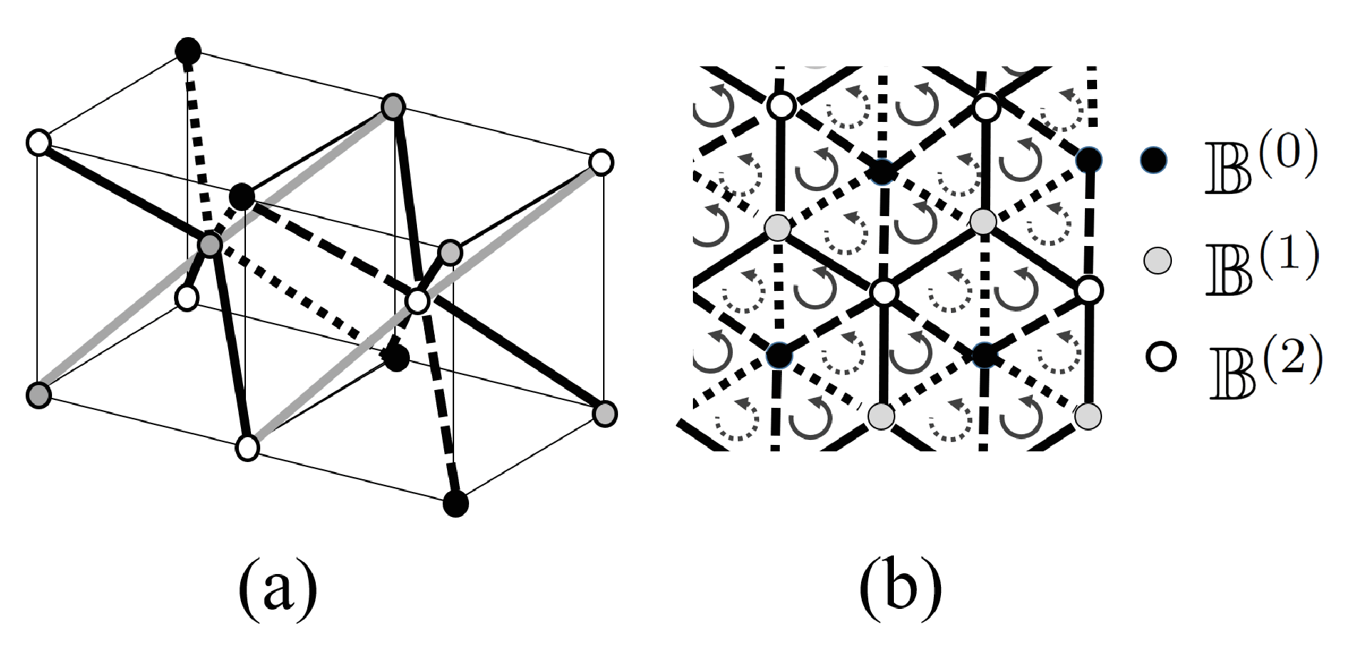
Figure 2. BCC lattice and its projection along the (1,1,1)(1,1,1)-direction: (a) shows the panoramic view of the unit cell of the BCC lattice which contains two triangles whose normal direction is (1,1,1)(1,1,1). (b) shows its projection along the (1,1,1)(1,1,1)-direction corresponding to (a).
Refer to caption
Figure 3. BCC lattice: The black, gray and white dots correspond to the three sheets 𝔹(0){\mathbb{B}}^{(0)}, 𝔹(1){\mathbb{B}}^{(1)} and 𝔹(2){\mathbb{B}}^{(2)}, which are associated with 𝒵BCC(0){\mathcal{Z}_{\mathrm{BCC}}^{(0)}}, 𝒵BCC(1){\mathcal{Z}_{\mathrm{BCC}}^{(1)}} and 𝒵BCC(2){\mathcal{Z}_{\mathrm{BCC}}^{(2)}} respectively.

The lattice 𝔹a{\mathbb{B}}^{a} is group-isomorphic to the multiplicative group

𝔹:={α1ℓ1α2ℓ2α3ℓ3βℓ4|abelian,ℓ1,ℓ2,ℓ3,ℓ4∈ℤ,β2α1−1α2−1α3−1=1}.{\mathbb{B}}:=\{\alpha_{1}^{\ell_{1}}\alpha_{2}^{\ell_{2}}\alpha_{3}^{\ell_{3}}\beta^{\ell_{4}}\,|\,\mbox{abelian},\ell_{1},\ell_{2},\ell_{3},\ell_{4}\in{\mathbb{Z}},\,\beta^{2}\alpha_{1}^{-1}\alpha_{2}^{-1}\alpha_{3}^{-1}=1\}.

Let us denote by 𝔸4{\mathbb{A}}_{4} the multiplicative free abelian group of rank 44 generated by α1\alpha_{1}, α2\alpha_{2}, α3\alpha_{3} and β\beta, i.e.,

𝔸4:={α1ℓ1α2ℓ2α3ℓ3βℓ4|abelian,ℓ1,ℓ2,ℓ3,ℓ4∈ℤ}.{\mathbb{A}}_{4}:=\{\alpha_{1}^{\ell_{1}}\alpha_{2}^{\ell_{2}}\alpha_{3}^{\ell_{3}}\beta^{\ell_{4}}\,|\,\mbox{abelian},\,\ell_{1},\ell_{2},\ell_{3},\ell_{4}\in{\mathbb{Z}}\}.

Then, 𝔹{\mathbb{B}} is also described as the quotient group

𝔹=𝔸4/⟨β2​α1−1​α2−1​α3−1⟩,{\mathbb{B}}={\mathbb{A}}_{4}/\langle\beta^{2}\alpha_{1}^{-1}\alpha_{2}^{-1}\alpha_{3}^{-1}\rangle,

where ⟨β2​α1−1​α2−1​α3−1⟩\langle\beta^{2}\alpha_{1}^{-1}\alpha_{2}^{-1}\alpha_{3}^{-1}\rangle is the (normal) subgroup generated by β2​α1−1​α2−1​α3−1\beta^{2}\alpha_{1}^{-1}\alpha_{2}^{-1}\alpha_{3}^{-1}. We shall consider the group ring ℂ⁡[𝔹]{\mathbb{C}}[{\mathbb{B}}] of 𝔹{\mathbb{B}},

ℛ6:=ℂ⁡[𝔹]=ℂ⁡[α1,α2,α3,α1−1,α2−1,α3−1,β,β−1]/(β2−α1​α2​α3).{\mathcal{R}}_{6}:={\mathbb{C}}[{\mathbb{B}}]={\mathbb{C}}[\alpha_{1},\alpha_{2},\alpha_{3},\alpha_{1}^{-1},\alpha_{2}^{-1},\alpha_{3}^{-1},\beta,\beta^{-1}]/(\beta^{2}-\alpha_{1}\alpha_{2}\alpha_{3}).

4.3. Algebraic Structure of BCC Lattice for (1,1,1)(1,1,1)-Direction

It is known that a screw dislocation in the BCC lattice is basically given by the (1,1,1)(1,1,1)-direction since the Burgers vector is parallel to the (1,1,1)(1,1,1)-direction [Na].

In this subsection, we consider the algebraic structure of the BCC lattice of (111)-direction to describe its fibering structure by noting Figure 2 (a) and (b). Let us consider the subgroup of 𝔹{\mathbb{B}}, which corresponds to the translation in the plane vertical to (1,1,1)(1,1,1)-direction,

𝔹H:={(α1α3−1)ℓ1(α2α3−1)ℓ2|ℓ1,ℓ2∈ℤ},{\mathbb{B}}_{H}:=\{(\alpha_{1}\alpha_{3}^{-1})^{\ell_{1}}(\alpha_{2}\alpha_{3}^{-1})^{\ell_{2}}\,|\,\ell_{1},\ell_{2}\in{\mathbb{Z}}\},

and ℂ⁡[𝔹H]{\mathbb{C}}[{\mathbb{B}}_{H}]-modules.

Lemma 4.4.

There are isomorphisms as ℂ⁡[𝔹H]{\mathbb{C}}[{\mathbb{B}}_{H}]-modules:

ℛ6/(α1​α2​α3−1)\displaystyle{\mathcal{R}}_{6}/(\alpha_{1}\alpha_{2}\alpha_{3}-1) ≅\displaystyle\cong ℂ⁡[𝔹H]⊕ℂ⁡[𝔹H]​α1⊕ℂ⁡[𝔹H]​α1​α2\displaystyle{\mathbb{C}}[{\mathbb{B}}_{H}]\oplus{\mathbb{C}}[{\mathbb{B}}_{H}]\alpha_{1}\oplus{\mathbb{C}}[{\mathbb{B}}_{H}]\alpha_{1}\alpha_{2}
⊕ℂ⁡[𝔹H]​β⊕ℂ⁡[𝔹H]​α1​β⊕ℂ⁡[𝔹H]​α1​α2​β.\displaystyle\quad\oplus{\mathbb{C}}[{\mathbb{B}}_{H}]\beta\oplus{\mathbb{C}}[{\mathbb{B}}_{H}]\alpha_{1}\beta\oplus{\mathbb{C}}[{\mathbb{B}}_{H}]\alpha_{1}\alpha_{2}\beta.
ℛ3:=ℛ6/(β−1)≅ℂ⁡[𝔹H]⊕ℂ⁡[𝔹H]​α1⊕ℂ⁡[𝔹H]​α1​α2.{\mathcal{R}}_{3}:={\mathcal{R}}_{6}/(\beta-1)\cong{\mathbb{C}}[{\mathbb{B}}_{H}]\oplus{\mathbb{C}}[{\mathbb{B}}_{H}]\alpha_{1}\oplus{\mathbb{C}}[{\mathbb{B}}_{H}]\alpha_{1}\alpha_{2}.

These decompositions mean that the BCC lattice has the triple different fiber structures of three sheets. We should note that ℛ6{\mathcal{R}}_{6} can be regarded as a double covering of ℛ3{\mathcal{R}}_{3}. The interval between the sheets is now given by 3​a/6\sqrt{3}a/6, and let us denote ℛ3{\mathcal{R}}_{3} as a set, the image of the forgetful functor to the category of set, by 𝔹a{\mathbb{B}}^{a} as a subset of the vector space ℝ3{\mathbb{R}}^{3} corresponding to the three sheets:

Lemma 4.5.

As a set, 𝔹a{\mathbb{B}}^{a} is also decomposed as

𝔹a=𝔹(0)​∐𝔹(1)​∐𝔹(2),{\mathbb{B}}^{a}={\mathbb{B}}^{(0)}\coprod{\mathbb{B}}^{(1)}\coprod{\mathbb{B}}^{(2)},

where

𝔹(0):={ℓ1(a1−a3)+ℓ2(a2−a3)+ℓ3b|ℓ1,ℓ2,ℓ3∈ℤ}⊂ℝ3,𝔹(1):={ℓ1(a1−a3)+ℓ2(a2−a3)+a1+ℓ3b|ℓ1,ℓ2,ℓ3∈ℤ}⊂ℝ3,𝔹(2):={ℓ1(a1−a3)+ℓ2(a2−a3)+a1+a2+ℓ3b|ℓ1,ℓ2,ℓ3∈ℤ}⊂ℝ3.\begin{array}[]{rl}{\mathbb{B}}^{(0)}&:=\{\ell_{1}(a_{1}-a_{3})+\ell_{2}(a_{2}-a_{3})+\ell_{3}b\,|\,\ell_{1},\ell_{2},\ell_{3}\in{\mathbb{Z}}\}\subset{\mathbb{R}}^{3},\\ {\mathbb{B}}^{(1)}&:=\{\ell_{1}(a_{1}-a_{3})+\ell_{2}(a_{2}-a_{3})+a_{1}+\ell_{3}b\,|\,\ell_{1},\ell_{2},\ell_{3}\in{\mathbb{Z}}\}\subset{\mathbb{R}}^{3},\\ {\mathbb{B}}^{(2)}&:=\{\ell_{1}(a_{1}-a_{3})+\ell_{2}(a_{2}-a_{3})+a_{1}+a_{2}+\ell_{3}b\,|\,\ell_{1},\ell_{2},\ell_{3}\in{\mathbb{Z}}\}\subset{\mathbb{R}}^{3}.\\ \end{array}

4.4. Fiber Structure of BCC Lattice and Eisenstein Integers

We can regard 𝔹(a){\mathbb{B}}^{(a)} as trivial covering space of ℓ3\ell_{3}-direction. On the other hand, the additive group of 𝔹H{\mathbb{B}}_{H},

𝔹Ha:={ℓ1(a1−a3)+ℓ2(a2−a3)|ℓ1,ℓ2∈ℤ}⊂ℝ2,{\mathbb{B}}_{H}^{a}:=\{\ell_{1}(a_{1}-a_{3})+\ell_{2}(a_{2}-a_{3})\,|\,\ell_{1},\ell_{2}\in{\mathbb{Z}}\}\subset{\mathbb{R}}^{2},

can be expressed by the the Eisenstein integers.

We define

d0:=32​a=|b|,d1:=2​a,d2:=13​d1=23​a,d3:=36​a=d03.d_{0}:=\frac{\sqrt{3}}{2}a=|b|,\quad d_{1}:=\sqrt{2}a,\quad d_{2}:=\frac{1}{\sqrt{3}}d_{1}=\frac{\sqrt{2}}{\sqrt{3}}a,\quad d_{3}:=\frac{\sqrt{3}}{6}a=\frac{d_{0}}{3}.

and 𝒵BCC(a):=(ℤ⁡[ω6]+μc)​d1{\mathcal{Z}_{\mathrm{BCC}}^{(a)}}:=({\mathbb{Z}}[\omega_{6}]+\mu_{c})d_{1} (a=0,1,2)(a=0,1,2) using (4.1), i.e.,

𝒵BCC(0)=ℤ⁡[ω6]​d1,𝒵BCC(1)=ℤ⁡[ω6]​d1+ν0​d1,𝒵BCC(2)=ℤ⁡[ω6]​d1+ν1​d1,{\mathcal{Z}_{\mathrm{BCC}}^{(0)}}={\mathbb{Z}}[\omega_{6}]d_{1},\quad{\mathcal{Z}_{\mathrm{BCC}}^{(1)}}={\mathbb{Z}}[\omega_{6}]d_{1}+\nu_{0}d_{1},\quad{\mathcal{Z}_{\mathrm{BCC}}^{(2)}}={\mathbb{Z}}[\omega_{6}]d_{1}+\nu_{1}d_{1},\quad

which correspond to 𝔹(0){\mathbb{B}}^{(0)}, 𝔹(1){\mathbb{B}}^{(1)} and 𝔹(2){\mathbb{B}}^{(2)} respectively as in Figure 3, i.e., there are natural projections for bb-direction, πBCC(a):𝔹(a)→𝒵BCC(a)\pi_{{\mathrm{BCC}}}^{(a)}:{\mathbb{B}}^{(a)}\to{\mathcal{Z}_{\mathrm{BCC}}^{(a)}}.

Remark 4.6.

The projection πBCC(a)\pi_{{\mathrm{BCC}}}^{(a)} of these 𝔹(0){\mathbb{B}}^{(0)}, 𝔹(1){\mathbb{B}}^{(1)} and 𝔹(2){\mathbb{B}}^{(2)} are essentially equal to ℤ⁡[ω6]{\mathbb{Z}}[\omega_{6}] up to translation and dilatation d1d_{1}. Further μc\mu_{c} and νi\nu_{i} are third points in the lattice νi∈13​ℤ​[ω6]\nu_{i}\in\frac{1}{3}{\mathbb{Z}}[\omega_{6}]. They have the algebraic properties of Lemmas 4.1 and 4.2 and Remark 4.3, whose origin in the ring of integers of the cyclotomic field ℚ⁡[ω6]{\mathbb{Q}}[\omega_{6}]. They have studied in the number theory and algebraic geometry [FKMPA, Appendix], and their application to physics [Ma].

As shown in the following, the z3z_{3} position of each sheet in the screw dislocations along the (1,1,1)(1,1,1)-direction and the local energy due to the dislocation can be regarded as functions on ℤ⁡[ω6]{\mathbb{Z}}[\omega_{6}], more precisely on 𝒵BCC(c):=(ℤ⁡[ω6]+μc)​d1{\mathcal{Z}_{\mathrm{BCC}}^{(c)}}:=({\mathbb{Z}}[\omega_{6}]+\mu_{c})d_{1} (c=0,1,2)(c=0,1,2). Thus Lemmas 4.1 and 4.2 govern the computations of the functions in Lemma 4.11 and make them very simple and connected with the Epstein-Hurwitz zeta function as in Theorem 4.14.

Though in the previous works including [HMNSU], such properties had not been mentioned, these properties show algebraic nature of the BCC lattice and the screw dislocation in the BCC lattice.

For a point δ=(δ1,δ2,δ3)∈𝔼3\delta=(\delta_{1},\delta_{2},\delta_{3})\in{\mathbb{E}}^{3}, we consider the embedding ιδ:𝔹a→𝔼3\iota_{\delta}:{\mathbb{B}}^{a}\to{\mathbb{E}}^{3} and its image ιδ​(𝔹a)\iota_{\delta}({\mathbb{B}}^{a}). Corresponding to ιδ\iota_{\delta}, for the point δℂ=δ1+−1​δ2∈𝔼ℂ\delta_{\mathbb{C}}=\delta_{1}+{\sqrt{-1}}\delta_{2}\in{\mathbb{E}}_{\mathbb{C}}, let us also consider the embedding ιδℂ:𝒵BCC(c)→𝒵BCC(c)+δℂ∈𝔼ℂ\iota_{\delta_{\mathbb{C}}}:{\mathcal{Z}_{\mathrm{BCC}}^{(c)}}\to{\mathcal{Z}_{\mathrm{BCC}}^{(c)}}+\delta_{\mathbb{C}}\in{\mathbb{E}}_{\mathbb{C}} and the bundle maps ι^δℂ\widehat{\iota}_{\delta_{\mathbb{C}}}. Further for γδ=e−1​δ3/d0∈S1\gamma_{\delta}=\mathrm{e}^{{\sqrt{-1}}\delta_{3}/d_{0}}\in S^{1} and a constant section 𝔲δ∈Γ⁡(𝔼ℂ,S𝔼ℂ1)\mathfrak{u}_{\delta}\in\Gamma({\mathbb{E}}_{\mathbb{C}},S^{1}_{{\mathbb{E}}_{\mathbb{C}}}) (𝔲δ​(z)=γδ)(\mathfrak{u}_{\delta}(z)=\gamma_{\delta}), we consider 𝔲δBCC∈Γ⁡(𝒵BCC,S𝒵BCC1)\mathfrak{u}^{\mathrm{BCC}}_{\delta}\in\Gamma({\mathcal{Z}_{\mathrm{BCC}}},S^{1}_{{\mathcal{Z}_{\mathrm{BCC}}}}) as

𝔲δBCC:=𝔲δ∘ιδℂ.\mathfrak{u}^{\mathrm{BCC}}_{\delta}:=\mathfrak{u}_{\delta}\circ\iota_{\delta_{\mathbb{C}}}.

where S𝒵BCC1S^{1}_{{\mathcal{Z}_{\mathrm{BCC}}}} is the trivial S1S^{1} bundle over 𝒵BCC{\mathcal{Z}_{\mathrm{BCC}}}.

Proposition 4.7.

The BCC lattice ιδ​(𝔹a)\iota_{\delta}({\mathbb{B}}^{a}) is expressed by

⋃c=02ι^δℂ​(ψ^d0−1​(ω3−c​𝔲δBCC​(𝒵BCC(c))))⊂𝔼𝔼ℂ=𝔼3.\bigcup_{c=0}^{2}\widehat{\iota}_{\delta_{\mathbb{C}}}\left(\widehat{\psi}_{d_{0}}^{-1}\left(\omega_{3}^{-c}\mathfrak{u}^{\mathrm{BCC}}_{\delta}({\mathcal{Z}_{\mathrm{BCC}}^{(c)}})\right)\right)\subset{\mathbb{E}}_{{\mathbb{E}}_{\mathbb{C}}}={\mathbb{E}}^{3}.

Here we set d=d0=|b|d=d_{0}=|b| of ψd\psi_{d} in Section 2.

4.5. Spiral Structure in Graph of BCC Lattice
Refer to caption
Figure 4. Spiral Structure in Graph of BCC Lattice: (a) is a panoramic view of a part of GδBCCG^{\mathrm{BCC}}_{\delta} consisting of two unit cells of the BCC lattice with edges, where the gray line shows the (1,1,1)(1,1,1)-direction, and the black lines means the edges of GδBCCG^{\mathrm{BCC}}_{\delta}. The edges drawn by the short dotted line, long dotted line and solid line corresponds to those of the projected graph πG​GδBCC\pi_{G}G^{\mathrm{BCC}}_{\delta} as in (b). The arrows of solid lines show the ascendant triangles whereas the arrows of dot lines correspond to the descendant triangles

In the BCC lattice ιδ​(𝔹a)\iota_{\delta}({\mathbb{B}}^{a}), let us consider the graph GδBCCG^{\mathrm{BCC}}_{\delta} whose nodes are given as the lattice points of the BCC lattice and edges are given as the shortest connections of the nodes as shown in Figure 4 (a). We regard GδBCCG^{\mathrm{BCC}}_{\delta} as a subset of 𝔼3{\mathbb{E}}^{3}. The 0-th sheet ιδ​(𝔹(0))\iota_{\delta}({\mathbb{B}}^{(0)}) (ιδℂ​(𝒵BCC(0))\iota_{\delta_{\mathbb{C}}}({\mathcal{Z}_{\mathrm{BCC}}^{(0)}})) whose nodes are denoted by the black dots is connected with the first sheet ιδ​(𝔹(1))\iota_{\delta}({\mathbb{B}}^{(1)}) (OPENιδℂ​𝒵BCC(1))\iota_{\delta_{\mathbb{C}}}{\mathcal{Z}_{\mathrm{BCC}}^{(1)}})) which corresponds to the gray dots, via the long dots lines in Figure 4 (a). The short dot line connects ιδ​(𝔹(2))\iota_{\delta}({\mathbb{B}}^{(2)}) (OPENιδℂ​𝒵BCC(2))\iota_{\delta_{\mathbb{C}}}{\mathcal{Z}_{\mathrm{BCC}}^{(2)}})) and ιδ​(𝔹(0))\iota_{\delta}({\mathbb{B}}^{(0)}) (OPENιδℂ​𝒵BCC(0))\iota_{\delta_{\mathbb{C}}}{\mathcal{Z}_{\mathrm{BCC}}^{(0)}})) whereas the black lines connect ιδ​(𝔹(1))\iota_{\delta}({\mathbb{B}}^{(1)}) (OPENιδℂ​𝒵BCC(1))\iota_{\delta_{\mathbb{C}}}{\mathcal{Z}_{\mathrm{BCC}}^{(1)}})) and ιδ​(𝔹(2))\iota_{\delta}({\mathbb{B}}^{(2)}) (OPENιδℂ​𝒵BCC(2))\iota_{\delta_{\mathbb{C}}}{\mathcal{Z}_{\mathrm{BCC}}^{(2)}})).

The graph GδBCCG^{\mathrm{BCC}}_{\delta} has a projection to a plane 𝔼ℂ{\mathbb{E}}_{\mathbb{C}} as in Figure 4 (b): πG:GδBCC→𝔼ℂ\pi_{G}:G^{\mathrm{BCC}}_{\delta}\to{\mathbb{E}}_{\mathbb{C}}, These edges give the paths which connect these covering sheets. As in Figure 4 (b), let us consider the path whose projection is a cycle πG​(GδBCC)\pi_{G}(G^{\mathrm{BCC}}_{\delta}) consisting of tree edges, which is called ”spiral path” because the end point pp and the start point qq exist on the different covering sheets but q∈πG−1​(πG​(p))q\in\pi_{G}^{-1}(\pi_{G}(p)); if the start point is (ℓ1,ℓ2,ℓ3)(\ell_{1},\ell_{2},\ell_{3}) in ιδ​(𝔹(a))\iota_{\delta}({\mathbb{B}}^{(a)}), the end point is given as (ℓ1,ℓ2,ℓ3′)(\ell_{1},\ell_{2},\ell_{3}^{\prime}) in ιδ​(𝔹(a))\iota_{\delta}({\mathbb{B}}^{(a)}) for |ℓ3′−ℓ3|=d0=|b||\ell_{3}^{\prime}-\ell_{3}|=d_{0}=|b|. Thus the path shows the spiral curve in 𝔼3{\mathbb{E}}^{3}.

The set of the spiral paths is classified by two types. We assign an orientation on 𝔼ℂ{\mathbb{E}}_{\mathbb{C}} and the orientation of the arrowed graph [πG​(GδBCC)][\pi_{G}(G^{\mathrm{BCC}}_{\delta})] is naturally induced from it. For the oriental cycle in πG​(GδBCC)\pi_{G}(G^{\mathrm{BCC}}_{\delta}), the spiral path is ascendant or decedent with respect to ℓ3\ell_{3}. We call these triangle cells ascendant cell and descendant cell respectively. They are illustrated in Figure 5 (a) and (b) respectively.

For a center point zcz_{c} of a ascendant triangle cell of πG​(GδBCC)\pi_{G}(G^{\mathrm{BCC}}_{\delta}), the nodes in GδBCCG^{\mathrm{BCC}}_{\delta} are given by

(4.2) ψd0−1​(γδ​z−zc|z−zc|),\psi_{d_{0}}^{-1}\left(\gamma_{\delta}\frac{z-z_{c}}{|z-z_{c}|}\right),

whereas for a center point zcz_{c} of a descendant triangle cell of πG​(GδBCC)\pi_{G}(G^{\mathrm{BCC}}_{\delta}), the nodes are expressed by

(4.3) ψd0−1​(γδ​z−zc¯|z−zc|).\psi_{d_{0}}^{-1}\left(\gamma_{\delta}\frac{\overline{z-z_{c}}}{|z-z_{c}|}\right).

These pictures are well-described in the works of Ramasubramaniam, Ariza and Ortiz [ARO] and [AO] using the homological investigations more precisely.

Refer to caption
Figure 5. Spiral Paths in BCC lattice: (a) and (c) are ascendant spiral paths and (b) and (d) decedent spiral paths. (a) and (b) are normal cases whereas (c) and (d) are the behavior when in the center, the screw dislocation exists.

4.6. Algebraic Description of Screw Dislocations in BCC Lattice

As defined in Subsection 4.5, for δ∈𝔼3\delta\in{\mathbb{E}}^{3} and z0∈𝔼ℂz_{0}\in{\mathbb{E}}_{\mathbb{C}}, we use the embedding ιδℂ:𝒵BCC(i)→𝒵BCC(i)+δℂ∈𝔼ℂ∖{z0}\iota_{\delta_{\mathbb{C}}}:{\mathcal{Z}_{\mathrm{BCC}}^{(i)}}\to{\mathcal{Z}_{\mathrm{BCC}}^{(i)}}+\delta_{\mathbb{C}}\in{\mathbb{E}}_{\mathbb{C}}\setminus\{z_{0}\}, δℂ=δ1+−1​δ2∈𝔼ℂ\delta_{\mathbb{C}}=\delta_{1}+{\sqrt{-1}}\delta_{2}\in{\mathbb{E}}_{\mathbb{C}}, γδ=e−1​δ3/d0∈S1\gamma_{\delta}=\mathrm{e}^{{\sqrt{-1}}\delta_{3}/d_{0}}\in S^{1} and the bundle map ψ^d0\widehat{\psi}_{d_{0}} so that the description of the screw dislocation is obtained as follows. Let us consider the non-trivial S1S^{1}-bundle over 𝒵BCC{\mathcal{Z}_{\mathrm{BCC}}} induced from the embedding ιδℂ\iota_{\delta_{\mathbb{C}}}. Using the section of 𝔲z0,δ∈Γ⁡(𝔼ℂ∖{z0},S𝔼ℂ∖{z0}1)\mathfrak{u}_{z_{0},\delta}\in\Gamma({\mathbb{E}}_{\mathbb{C}}\setminus\{z_{0}\},S^{1}_{{\mathbb{E}}_{\mathbb{C}}\setminus\{z_{0}\}}) in (2.5), we define the section 𝔲^z0,δ\widehat{\mathfrak{u}}_{z_{0},\delta} in Γ⁡(𝒵BCC,S𝒵BCC1)\Gamma({\mathcal{Z}_{\mathrm{BCC}}},S^{1}_{{\mathcal{Z}_{\mathrm{BCC}}}}),

𝔲z0,δBCC=ιδℂ∗​𝔲δ,z0=𝔲z0,δ∘ιδℂ.\mathfrak{u}^{\mathrm{BCC}}_{z_{0},\delta}=\iota^{*}_{\delta_{\mathbb{C}}}\mathfrak{u}_{\delta,z_{0}}=\mathfrak{u}_{z_{0},\delta}\circ\iota_{\delta_{\mathbb{C}}}.

It implies that

𝔲z0,δBCC(ℓd1)=γδd1​ℓ+δℂ−z0|d1​ℓ+δℂ−z0|,for ℓd1∈𝒵BCC(c).(c=0,1,2).\mathfrak{u}^{\mathrm{BCC}}_{z_{0},\delta}(\ell d_{1})=\gamma_{\delta}\frac{d_{1}\ell+\delta_{\mathbb{C}}-z_{0}}{|d_{1}\ell+\delta_{\mathbb{C}}-z_{0}|},\qquad\mbox{\rm for }\ell d_{1}\in{\mathcal{Z}_{\mathrm{BCC}}^{(c)}}.\quad(c=0,1,2).
Proposition 4.8.

The single screw dislocation around π𝔼−1​(z0)⊂𝔼3=𝔼𝔼ℂ\pi_{{\mathbb{E}}}^{-1}(z_{0})\subset{\mathbb{E}}^{3}={\mathbb{E}}_{{\mathbb{E}}_{\mathbb{C}}} expressed by

⋃c=02ι^δℂ​(ψ^d0−1​(ω3−c​𝔲z0,δBCC​(𝒵BCC(c))))\bigcup_{c=0}^{2}\widehat{\iota}_{\delta_{\mathbb{C}}}\left(\widehat{\psi}_{d_{0}}^{-1}\left(\omega_{3}^{-c}\mathfrak{u}^{\mathrm{BCC}}_{z_{0},\delta}({\mathcal{Z}_{\mathrm{BCC}}^{(c)}})\right)\right)

is a subset of 𝔼3{\mathbb{E}}^{3}.

Proof.

𝔼𝔼∖{z0}{\mathbb{E}}_{{\mathbb{E}}\setminus\{z_{0}\}} is obviously a subset of 𝔼3=𝔼𝔼ℂ{\mathbb{E}}^{3}={\mathbb{E}}_{{\mathbb{E}}_{\mathbb{C}}}. ∎

Remark 4.9.

Though it is obvious that the screw dislocation exists in 𝔼3{\mathbb{E}}^{3} in physics, it is not obvious that a geometrical object constructed in algebraic topology is realized in 𝔼3{\mathbb{E}}^{3}, e.g, the Klein bottle. Proposition 4.8 is crucial in the description of the physical object in terms of algebraic language.

As in the SC lattice, we also consider the graph Gz0,δBCCG_{z_{0},\delta}^{\mathrm{BCC}}. In the following, we also assume that γ=1\gamma=1 and δℂ=0\delta_{\mathbb{C}}=0 for simplicity.

4.7. Note on the Core Region of Screw Dislocations in BCC Lattice

Though the core structure in the screw dislocations in the BCC lattices has been studied well, e.g., in [Ta, ARO, AATMO] and using the first principle approach [Cl, GD, IKY], we show the description of the core region in terms of our framework.

Noting the equations (4.2) and (4.3), we consider the core region of the screw dislocation. The core region is the cells neighborhood of z0z_{0}.

If z0z_{0} is the center of the ascendant triangle, for a vertex zz of the triangle, the set of the fiber direction is

D⁡(z)=ψd0−1​(γδ​(z−zc)2|z−zc|2)=ψd0−1​(γδ​z−zcz−zc¯).D(z)=\psi_{d_{0}}^{-1}\left(\gamma_{\delta}\frac{(z-z_{c})^{2}}{|z-z_{c}|^{2}}\right)=\psi_{d_{0}}^{-1}\left(\gamma_{\delta}\frac{z-z_{c}}{\overline{z-z_{c}}}\right).

On the other hand, if z0z_{0} is the center of the decedent triangle, the set of the fiber direction is

D⁡(z)=ψd0−1​(γδ)D(z)=\psi_{d_{0}}^{-1}\left(\gamma_{\delta}\right)

for each vertex zz of the triangle. They are illustrated in Figure 5 (c) and (d) respectively. In the former case, there might exist different connections illustrated by the dotted lines. Thus the screw dislocation in the BCC lattice shows the quite different aspect from the case of the SC lattice.

The operation in Remark 2.3 can be applied to this system so that we have Figure 5 (c) and (d). By the operation, the connected spiral paths are deformed the disjointed paths. The disjoint subgraphs characterize the direction of the screw dislocations.

4.8. Energy of Screw Dislocation in BCC Lattice

In this section, we estimate the stress energy of the screw dislocation in the BCC lattice in the meso-scopic scale. We basically investigate the energy in parallel with the computations in the SC lattice.

For simply convention, we denote 𝔲z0,δBCC\mathfrak{u}^{\mathrm{BCC}}_{z_{0},\delta} etc. simply by 𝔲z0BCC\mathfrak{u}^{\mathrm{BCC}}_{z_{0}} etc. by suppressing δ\delta.

For ℓ∈ℤ⁡[ω6]+μc\ell\in{\mathbb{Z}}[\omega_{6}]+\mu_{c} (c=0,1,2)(c=0,1,2), we define the relative height differences εℓ(c,j)\varepsilon_{\ell}^{(c,j)} (j=0,1,⋯,5)(j=0,1,\cdots,5),

(4.4) εℓ(c,j)=d02​π​−1​(log⁡(𝔲z0BCC​((ℓ+νj)​d1)−log⁡(𝔲z0BCC​(ℓ​d1)))CLOSE=d04​π​−1​(log⁡(1+d1​νjℓ​d1−z0)−log⁡(1+d1​νj¯ℓ​d1−z0¯)).\begin{split}\varepsilon_{\ell}^{(c,j)}&=\frac{d_{0}}{2\pi{\sqrt{-1}}}\left(\log(\mathfrak{u}^{\mathrm{BCC}}_{z_{0}}((\ell+\nu_{j})d_{1})-\log(\mathfrak{u}^{\mathrm{BCC}}_{z_{0}}(\ell d_{1}))\right)\\ &=\frac{d_{0}}{4\pi{\sqrt{-1}}}\left(\log\left(1+\frac{d_{1}\nu_{j}}{\ell d_{1}-z_{0}}\right)-\log\left(1+\frac{\overline{d_{1}\nu_{j}}}{\overline{\ell d_{1}-z_{0}}}\right)\right).\end{split}

Here we require that −d3/2<εℓ(c,j)<d3/2-d_{3}/2<\varepsilon_{\ell}^{(c,j)}<d_{3}/2. Let us introduce a parameter ε>0\varepsilon>0 and using it, we define the core region Cε,IBCC⁡(j)C^{{\mathrm{BCC}}(j)}_{\varepsilon,I} of type I,

Cε,IBCC⁡(c):={ℓ∈ℤ[ω6]+μc|j∃=0,1,⋯,5 such that |εℓ(c,j)|>ε}.C^{{\mathrm{BCC}}(c)}_{\varepsilon,\mathrm{I}}:=\{\ell\in{\mathbb{Z}}[\omega_{6}]+\mu_{c}\ |\ {}^{\exists}{j}=0,1,\cdots,5\mbox{ such that }|\varepsilon_{\ell}^{(c,j)}|>\varepsilon\}.

Assume that ε<d3/2\varepsilon<d_{3}/2. The difference of length in each segment between ℓ∈𝒵BCC(c)∖d1​Cε,IBCC⁡(c)\ell\in{\mathcal{Z}_{\mathrm{BCC}}^{(c)}}\setminus d_{1}C^{{\mathrm{BCC}}(c)}_{\varepsilon,\mathrm{I}} and its nearest neighbor lattice points is given by

Δℓ(c,j)=(d3+(−1)j​εℓ(c,j))2+d22−d32+d22,\Delta_{\ell}^{(c,j)}=\sqrt{\left(d_{3}+(-1)^{j}\varepsilon_{\ell}^{(c,j)}\right)^{2}+d_{2}^{2}}-\sqrt{d_{3}^{2}+d_{2}^{2}},

for j=0,1,⋯,5j=0,1,\cdots,5. Here we note that d32+d22=3​a/2=d0\sqrt{d_{3}^{2}+d_{2}^{2}}=\sqrt{3}a/2=d_{0}.

We have the following.

Lemma 4.10.

If d1|ℓ​d1−z0|2\displaystyle{\frac{d_{1}}{\sqrt{|\ell d_{1}-z_{0}|^{2}}}} for an ℓ∈ℤ⁡[ω6]+μc\ell\in{\mathbb{Z}}[\omega_{6}]+\mu_{c} (c=0,1,2)(c=0,1,2) is sufficiently small, εℓ(c,j)\varepsilon^{(c,j)}_{\ell}’s are approximated by

(4.5) εℓ(c,j)=d0​d14​π​−1​(νjℓ​d1−z0−νj¯(ℓ​d1−z0)¯)+o⁡(d1|ℓ​d1−z0|2),\varepsilon_{\ell}^{(c,j)}=\frac{d_{0}d_{1}}{4\pi{\sqrt{-1}}}\left(\frac{\nu_{j}}{\ell d_{1}-z_{0}}-\frac{\overline{\nu_{j}}}{\overline{(\ell d_{1}-z_{0})}}\right)+o\left(\frac{d_{1}}{\sqrt{|\ell d_{1}-z_{0}|^{2}}}\right),

respectively, whereas Δℓ(c,j)\Delta_{\ell}^{(c,j)} are approximated by

(4.6) Δℓ(c,j)=(−1)j​d3d0​εℓ(c,j)+o⁡(d1|ℓ​d1−z0|2).\displaystyle{\Delta_{\ell}^{(c,j)}=\frac{(-1)^{j}d_{3}}{d_{0}}\varepsilon_{\ell}^{(c,j)}+o\left(\frac{d_{1}}{\sqrt{|\ell d_{1}-z_{0}|^{2}}}\right).}
Proof.

Noting log⁡(1+z)=z+o⁡(z2)\log(1+z)=z+o(z^{2}), 1+z−1=12​z+o⁡(z2)\displaystyle{\sqrt{1+z}-1=\frac{1}{2}z+o(z^{2})}, d32+d23=3​a/2=d0\sqrt{d_{3}^{2}+d_{2}^{3}}=\sqrt{3}a/2=d_{0}, the direct computations show them. ∎

As mentioned in Remark 4.6, due to the properties of the Eisenstein integers ℤ⁡[ωg]{\mathbb{Z}}[\omega_{g}] in Lemmas 4.1 and 4.2, we have the simple expression:

Lemma 4.11.

If d1|ℓ​d1−z0|2\displaystyle{\frac{d_{1}}{\sqrt{|\ell d_{1}-z_{0}|^{2}}}} for an ℓ∈ℤ⁡[ω6]+μc\ell\in{\mathbb{Z}}[\omega_{6}]+\mu_{c} (c=0,1,2)(c=0,1,2) is sufficiently small,

(4.7) 12​∑j=05(Δℓ(c,j))2=1384​π2​d14|ℓ​d1−z0|2+o⁡(d1|ℓ​d1−z0|23).\frac{1}{2}\sum_{j=0}^{5}(\Delta_{\ell}^{(c,j)})^{2}=\frac{1}{384\pi^{2}}\frac{d_{1}^{4}}{|\ell d_{1}-z_{0}|^{2}}+o\left(\frac{d_{1}}{\sqrt{|\ell d_{1}-z_{0}|^{2}}^{3}}\right).
Proof.

The left hand side is equal to

−12d02​d12​d3216​π2​d02∑j=05(νjℓ​d1−z0−νj¯ℓ​d1−z0¯)2+o(d1|ℓ​d1−z0|23),-\frac{1}{2}\frac{d_{0}^{2}d_{1}^{2}d_{3}^{2}}{16\pi^{2}d_{0}^{2}}\sum_{j=0}^{5}\left(\frac{\nu_{j}}{\ell d_{1}-z_{0}}-\frac{\overline{\nu_{j}}}{\overline{\ell d_{1}-z_{0}}}\right)^{2}+o\left(\frac{d_{1}}{\sqrt{|\ell d_{1}-z_{0}|^{2}}^{3}}\right),

and thus using Lemmas 4.1 and 4.2, it becomes

=d14384​π2​1|ℓ​d1−z0|2+o⁡(d1|ℓ​d1−z0|23).=\frac{d_{1}^{4}}{384\pi^{2}}\frac{1}{|\ell d_{1}-z_{0}|^{2}}+o\left(\frac{d_{1}}{\sqrt{|\ell d_{1}-z_{0}|^{2}}^{3}}\right).

Here the extra terms are canceled due to the properties of 13​ℤ​[ω6]\frac{1}{3}{\mathbb{Z}}[\omega_{6}]. ∎

Remark 4.12.

As we show in Remark 3.3, εℓ(c,j)\varepsilon_{\ell}^{(c,j)} is a real analytic function of wj:=d1​νjℓ​d1−z0\displaystyle{w_{j}:=\frac{d_{1}\nu_{j}}{\ell d_{1}-z_{0}}} and w¯j\overline{w}_{j} for |wj|≪1|w_{j}|\ll 1, i.e.,

εℓ(c,j)=εℓ​(wj,wj¯)=d04​π​−1​log⁡(1+wj1+wj¯),\varepsilon_{\ell}^{(c,j)}=\varepsilon_{\ell}(w_{j},\overline{w_{j}})=\frac{d_{0}}{4\pi{\sqrt{-1}}}\log\left(\frac{1+w_{j}}{\overline{1+w_{j}}}\right),

and thus Δℓ(c,j)\Delta_{\ell}^{(c,j)} is also a real analytic function of ww and w¯\overline{w}.

As we mentioned in Remark 4.3, we have the cyclotomic symmetry in ℤ⁡[ω6]{\mathbb{Z}}[\omega_{6}], or ℭ6{\mathfrak{C}}_{6} action on ℤ⁡[ω6]{\mathbb{Z}}[\omega_{6}]; there is the element g∈ℭ6g\in{\mathfrak{C}}_{6} such that g​νj=νj+1g\nu_{j}=\nu_{j+1} whose index is given modulo 6. The action induces the action on the function ff over ℤ⁡[ω6]{\mathbb{Z}}[\omega_{6}], i.e., g∗​f​(x)=f⁡(g​x)g^{*}f(x)=f(gx). By fixing ℓ​d1−z0\ell d_{1}-z_{0}, the action is given as

g∗​εℓ(c,j)=g∗​εℓ​(wj,wj¯)=εℓ(c,j+1),g^{*}\varepsilon_{\ell}^{(c,j)}=g^{*}\varepsilon_{\ell}(w_{j},\overline{w_{j}})=\varepsilon_{\ell}^{(c,j+1)},

and ∑j=05(Δℓ(c,j))2\displaystyle{\sum_{j=0}^{5}(\Delta_{\ell}^{(c,j)})^{2}} in Lemma 4.11 is invariant for the action g∈ℭ6g\in{\mathfrak{C}}_{6}.

For a positive number ρ\rho, let us define another core region Cρ,IIBCC⁡(c)C^{{\mathrm{BCC}}(c)}_{\rho,\mathrm{II}} of type II,

Cρ,IIBCC⁡(c):={ℓ∈ℤ⁡[ω6]+μc||ℓ​d1−z0|<ρ​d1}.C^{{\mathrm{BCC}}(c)}_{\rho,\mathrm{II}}:=\left\{\ell\in{\mathbb{Z}}[\omega_{6}]+\mu_{c}\ |\ \left|\ell d_{1}-z_{0}\right|<\rho d_{1}\right\}.

In order to avoid to count doubly, we should concentrate one of 𝒵BCC(c){\mathcal{Z}_{\mathrm{BCC}}^{(c)}}’s and choose 𝒵BCC(0){\mathcal{Z}_{\mathrm{BCC}}^{(0)}} in this paper. Let the core region of type III and its compliments be

Cε,ρ,IIIBCC⁡(0):={ℓ∈ℤ⁡[ω6]|ℓ∈Cε,IBCC⁡(0)∪Cρ,IIBCC⁡(0)​ or ​Ad​(ℓ​d1)⊂⋃c=12Cε,IBCC⁡(c)}C^{{\mathrm{BCC}}(0)}_{\varepsilon,\rho,\mathrm{III}}:=\{\ell\in{\mathbb{Z}}[\omega_{6}]\ |\ \ell\in C^{{\mathrm{BCC}}(0)}_{\varepsilon,\mathrm{I}}\cup C^{{\mathrm{BCC}}(0)}_{\rho,\mathrm{II}}\mbox{ or }\mathrm{Ad}(\ell d_{1})\subset\bigcup_{c=1}^{2}C^{{\mathrm{BCC}}(c)}_{\varepsilon,\mathrm{I}}\}

and

Aε,ρω6:=ℤ[ω6]∖Cε,ρ,IIIBCC⁡(0),Aε,ρ,Nω6:={ℓ∈Aε,ρω6||distz0(Ad(ℓd1)|<Nd1}.A^{\omega_{6}}_{\varepsilon,\rho}:={\mathbb{Z}}[\omega_{6}]\setminus C^{{\mathrm{BCC}}(0)}_{\varepsilon,\rho,\mathrm{III}},\qquad A^{\omega_{6}}_{\varepsilon,\rho,N}:=\{\ell\in A^{\omega_{6}}_{\varepsilon,\rho}\ |\ |\mathrm{dist}_{z_{0}}(\mathrm{Ad}(\ell d_{1})|<Nd_{1}\}.

where for a node vv in the plane graph πG​(Gz0BCC)\pi_{G}(G_{z_{0}}^{\mathrm{BCC}}), we denote the set of the adjacent nodes of vv by Ad⁡(v)\mathrm{Ad}(v) and we define

distz0​({vi}):=maxv∈{vi}⁡|v−z0|.\mathrm{dist}_{z_{0}}(\{v_{i}\}):=\max_{v\in\{v_{i}\}}|v-z_{0}|.

For the case that ρ\rho is sufficiently large for given ε(<d32)\varepsilon\displaystyle{\left(<\frac{d_{3}}{2}\right)} so that Cε,ρ,IIIBCC⁡(0)⊂Cρ,IIBCC⁡(0)C^{{\mathrm{BCC}}(0)}_{\varepsilon,\rho,\mathrm{III}}\subset C^{{\mathrm{BCC}}(0)}_{\rho,\mathrm{II}}, we also define

Aρω6:=Aε,ρω6,Aρ,Nω6:=Aε,ρ,Nω6.A^{\omega_{6}}_{\rho}:=A^{\omega_{6}}_{\varepsilon,\rho},\quad A^{\omega_{6}}_{\rho,N}:=A^{\omega_{6}}_{\varepsilon,\rho,N}.

We compute the stress energy caused by the screw dislocation in the BCC lattice as in the SC lattice case. We compute the energy density for unit length in the (1,1,1)(1,1,1)-direction, and call it simply the stress energy of dislocation again.

Let kdk_{d} be the spring constant of the edges. The stress energy of dislocation in the annulus region Aε,ρ,Nω6A^{\omega_{6}}_{\varepsilon,\rho,N} is given by

(4.8) Eε,ρ,NBCC​(z0):=∑ℓ∈Aε,ρ,Nω6ℰℓBCC,E^{\mathrm{BCC}}_{\varepsilon,\rho,N}(z_{0}):=\sum_{\ell\in A^{\omega_{6}}_{\varepsilon,\rho,N}}{\mathcal{E}}^{\mathrm{BCC}}_{\ell},

where ℰℓBCC{\mathcal{E}}^{\mathrm{BCC}}_{\ell} for every ℓ∈ℤ⁡[ω6]\ell\in{\mathbb{Z}}[\omega_{6}] is the energy density defined by

(4.9) ℰℓBCC:=12​kd​∑j=05(Δℓ(j))2.{\mathcal{E}}^{\mathrm{BCC}}_{\ell}:=\frac{1}{2}k_{d}\sum_{j=0}^{5}\left(\Delta_{\ell}^{(j)}\right)^{2}.

As in Proposition 3.7 in the SC lattice, we summarize the above results as the stress energy of the dislocation of the BCC lattice case:

Proposition 4.13.
  • (1)(1)

    For ℓ∈Aε,ρ,Nω6\ell\in A^{\omega_{6}}_{\varepsilon,\rho,N}, the energy density ℰℓ{\mathcal{E}}_{\ell} is expressed by a real analytic function ℰBCC​(w,w¯){\mathcal{E}}^{\mathrm{BCC}}(w,\overline{w}) of ww and w¯∈ℂ\bar{w}\in{\mathbb{C}} with |w|<1/2|w|<1/\sqrt{2} in such a way that

    ℰℓBCC=ℰBCC​(d1ℓ​d1−z0,d1ℓ​d1−z0¯).{\mathcal{E}}^{\mathrm{BCC}}_{\ell}={\mathcal{E}}^{\mathrm{BCC}}\left(\frac{d_{1}}{\ell d_{1}-z_{0}},\frac{d_{1}}{\overline{\ell d_{1}-z_{0}}}\right).
  • (2)(2)

    Let us consider the power series expansion

    ℰBCC​(w,w¯)=∑s=0∞ℰBCC(s)​(w,w¯),ℰBCC(s)​(w,w¯):=∑i+j=s,i,j≥0Ci,j​wi​w¯j,{\mathcal{E}}^{\mathrm{BCC}}(w,\overline{w})=\sum_{s=0}^{\infty}{\mathcal{E}}_{\mathrm{BCC}}^{(s)}(w,\overline{w}),\quad{\mathcal{E}}_{\mathrm{BCC}}^{(s)}(w,\overline{w}):=\sum_{i+j=s,i,j\geq 0}C_{i,j}w^{i}\overline{w}^{j},

    for some Ci,j∈ℂC_{i,j}\in{\mathbb{C}}. Then, we have the following:

    • (a)

      ℰBCC(0)​(w,w¯)=ℰBCC(1)​(w,w¯)=0{\mathcal{E}}_{\mathrm{BCC}}^{(0)}(w,\overline{w})={\mathcal{E}}_{\mathrm{BCC}}^{(1)}(w,\overline{w})=0,

    • (b)

      the leading term is given by

      (4.10) ℰBCC(2)​(w,w¯)=d14384​π2​kd​w​w¯,ℰBCC(2)​(d1ℓ​d1−z0,d1ℓ​d1−z0¯)=1384​π2​kd​[d14|ℓ​d1−z0|2],{\mathcal{E}}_{\mathrm{BCC}}^{(2)}(w,\overline{w})=\frac{d_{1}^{4}}{384\pi^{2}}k_{d}w\overline{w},\qquad{\mathcal{E}}_{\mathrm{BCC}}^{(2)}\left(\frac{d_{1}}{\ell d_{1}-z_{0}},\frac{d_{1}}{\overline{\ell d_{1}-z_{0}}}\right)=\frac{1}{384\pi^{2}}k_{d}\left[\frac{d_{1}^{4}}{|\ell d_{1}-z_{0}|^{2}}\right],
    • (c)

      Ci,j=Cj,i¯C_{i,j}=\overline{C_{j,i}}, and

    • (d)

      for every s≥2s\geq 2, there is a constant Ms>0M_{s}>0 such that

      |ℰBCC(s)​(w,w¯)|≤Ms​|w|s.|{\mathcal{E}}_{\mathrm{BCC}}^{(s)}(w,\overline{w})|\leq M_{s}|w|^{s}.
Proof.

Remark 4.12 Lemmas 4.10 and 4.11 show (1) and (2) (a), (b). Since the energy density is a real number, we obtain the relation in item (c). The analyticity in item (1) implies (d). This completes the proof. ∎

As the summation in (4.8) is finite, we have

(4.11) Eε,ρ,NBCC​(z0)=∑s=2∞∑ℓ∈Aε,ρ,Nω6ℰBCC(s)​(d1ℓ​d1−z0,d1ℓ​d1−z0¯).E^{\mathrm{BCC}}_{\varepsilon,\rho,N}(z_{0})=\sum_{s=2}^{\infty}\sum_{\ell\in A^{\omega_{6}}_{\varepsilon,\rho,N}}{\mathcal{E}}_{\mathrm{BCC}}^{(s)}\left(\frac{d_{1}}{\ell d_{1}-z_{0}},\frac{d_{1}}{\overline{\ell d_{1}-z_{0}}}\right).

In particular, we have the following theorem for the “principal part” of the stress energy.

Theorem 4.14.

For the case that ρ\rho is sufficiently large for given ε(<d32)\varepsilon\displaystyle{\left(<\frac{d_{3}}{2}\right)} so that Cε,ρ,IIIBCC⁡(0)⊂Cρ,IIBCC⁡(0)C^{{\mathrm{BCC}}(0)}_{\varepsilon,\rho,\mathrm{III}}\subset C^{{\mathrm{BCC}}(0)}_{\rho,\mathrm{II}}. Let Aρ,Nω6:=Aε,ρ,Nω6A^{\omega_{6}}_{\rho,N}:=A^{\omega_{6}}_{\varepsilon,\rho,N}. The principal part of the stress energy Eρ,N​(z0)E_{\rho,N}(z_{0}), defined by

Eρ,NBCC⁡(p)​(z0)\displaystyle E^{{\mathrm{BCC}}(\mathrm{p})}_{\rho,N}(z_{0}) :⁣=\displaystyle:= ∑ℓ∈Aρ,Nω6ℰBCC(2)​(d1ℓ​d1−z0,d1ℓ​a−z0¯)\displaystyle\sum_{\ell\in A^{\omega_{6}}_{\rho,N}}{\mathcal{E}}_{\mathrm{BCC}}^{(2)}\left(\frac{d_{1}}{\ell d_{1}-z_{0}},\frac{d_{1}}{\overline{\ell a-z_{0}}}\right)
=\displaystyle= 1384​π2​kd​∑ℓ∈Aρ,Nω6[d14|ℓ​d1−z0|2],\displaystyle\frac{1}{384\pi^{2}}k_{d}\sum_{\ell\in A^{\omega_{6}}_{\rho,N}}\left[\frac{d_{1}^{4}}{|\ell d_{1}-z_{0}|^{2}}\right],

is given by the truncated Epstein-Hurwitz zeta function (see Appendix),

(4.12) Eρ,NBCC⁡(p)(z0)=1384​π2kdd12ζρ,Nω6(2,−z0/d1).E^{{\mathrm{BCC}}(\mathrm{p})}_{\rho,N}(z_{0})=\frac{1}{384\pi^{2}}k_{d}d_{1}^{2}\zeta_{\rho,N}^{\omega_{6}}(2,-z_{0}/d_{1}).

It is noted that this theorem is obtained due to the properties of 13​ℤ​[ω6]\displaystyle{\frac{1}{3}{\mathbb{Z}}[\omega_{6}]} cf. Remark 4.6.

By Proposition 4.13 (2) (d), we can estimate each of the other terms appearing in the power series expansion (4.11) by the truncated Epstein-Hurwitz zeta function for Eisenstein integers as follows.

Proposition 4.15.

For each s≥3s\geq 3, there exists a positive constant Ms′M_{s}^{\prime} such that

(4.13) ∑ℓ∈Aρ,Nω6ℰBCC(s)(d1ℓ​d1−z0,d1ℓ​d1−z0¯)≤Ms′ζAρ,Nω6ω6(s,−z0/d1).\sum_{\ell\in A^{\omega_{6}}_{\rho,N}}{\mathcal{E}}_{\mathrm{BCC}}^{(s)}\left(\frac{d_{1}}{\ell d_{1}-z_{0}},\frac{d_{1}}{\overline{\ell d_{1}-z_{0}}}\right)\leq M_{s}^{\prime}\zeta_{A_{\rho,N}^{\omega_{6}}}^{\omega_{6}}(s,-z_{0}/d_{1}).

5. Discussion

In this paper, we investigated the screw dislocations of the SC lattice and the BCC lattice using the number theoretic descriptions in terms of the Gauss integers ℤ⁡[−1]{\mathbb{Z}}[{\sqrt{-1}}] and the Eisenstein integers ℤ⁡[ω6]{\mathbb{Z}}[\omega_{6}].

As mentioned in Remark 4.6, using the properties of the Eisenstein integers ℤ⁡[ω6]{\mathbb{Z}}[\omega_{6}], e.g., Lemmas 4.1 and 4.2, we obtain the simple description of the stress energy for the screw dislocation for the finite region except the core region. It reflects the symmetry of the screw dislocations. It is quite natural to investigate the symmetry of a mathematical object using algebraic language. Without the representation of the dislocation in terms of the Eisenstein integers ℤ⁡[ω6]{\mathbb{Z}}[\omega_{6}], it is very difficult to obtain the result because the dislocation in the BCC lattice is very complicate. Even for the core region, we can investigate it as in Subsection 4.7 using the properties of ℤ⁡[ω6]{\mathbb{Z}}[\omega_{6}]. Our description is natural even when we consider the analytic property like the energy minimum point of the screw dislocations because the symmetry is built in the descriptions.

We could estimate the dislocation of meso-scopic scale because the stress energy EtotalE_{\mathrm{total}} is given by

Etotal=Ecore+Emeso.E_{\mathrm{total}}=E_{\mathrm{core}}+E_{\mathrm{meso}}.

The effect in the core region should be investigated by the first principle computations but the meso-scopic energy could not be obtained. Even though we need more precise investigation for the estimation because there are some parameters, we have the formula to evaluate the meso-scopic energy. It is noted that the core energy is determined by the local data whereas the meso-scopic energy is determined by the meso-scopic data.

Refer to caption
Figure 6. The graph of ζρ,Nτ​(2,0)\zeta_{\rho,N}^{\tau}(2,0) v.s. log⁡N\log N for ρ=5.1\rho=5.1

The energy of the meso-scale essentially diverges and thus it is important to determine the cut-off parameter NN. Let ζρ,Nτ​(s,z0):=ζAρ,Nττ​(s,z0)\zeta_{\rho,N}^{\tau}(s,z_{0}):=\zeta_{A_{\rho,N}^{\tau}}^{\tau}(s,z_{0}). As we show the behaviors of the ζρ,Nτ​(2,0)\zeta_{\rho,N}^{\tau}(2,0) for τ=−1\tau={\sqrt{-1}} and ω6\omega_{6} in Figure 6, they are approximated well by the logarithmic function. It is natural since the continuum theory, in which the dislocation energy Etotal​(R)E_{\mathrm{total}}(R) in the inner region {z∈ℂ||z−z0|<R}\{z\in{\mathbb{C}}\ ||z-z_{0}|<R\} is written by the logarithmic function with respect to the radius from the dislocation line; Etotal​(R)∝log⁡RE_{\mathrm{total}}(R)\propto\log R.

Further we show the density of the ζρ,Nτ​(2,x+y​τ′)\zeta_{\rho,N}^{\tau}(2,x+y\tau^{\prime}) as in Figure 7 by numerical computations; the region of z0/dz_{0}/d is divided by 20×2020\times 20 blocks. These aspects in the regions are different though the differences are not large due to the divergent properties like the logarithmic function.

Refer to caption
Figure 7. The graph of ζρ,Nτ​(2,x+y​τ′)\zeta_{\rho,N}^{\tau}(2,x+y\tau^{\prime}) for. (ρ,N)=(7.2,75)(\rho,N)=(7.2,75): (a) ζρ,N−1​(2,x+y​−1)\zeta_{\rho,N}^{\sqrt{-1}}(2,x+y{\sqrt{-1}}) with gray scale: black = 14.664, white = 14.779 and (b) ζρ,Nω6​(2,x+y​ω6)\zeta_{\rho,N}^{\omega_{6}}(2,x+y\omega_{6}) with gray scale: black =16.061, white = 16.907

As we computed the double dislocations case in the SC lattice in the previous work [HMNSU, Appendix], they are described well by the Green function in the statistical field theory like vortexes as in [AO, ID]. In the computations of the Green function, there appear the quadratic form k​ℓ∈ℂk\ell\in{\mathbb{C}} modulo 2​π​ℤ2\pi{\mathbb{Z}}, where k∈ℚ⁡(τ)​π/dk\in{\mathbb{Q}}(\tau)\pi/d and ℓ∈ℤ⁡(τ)​d\ell\in{\mathbb{Z}}(\tau)d for d=ad=a or d=d1d=d_{1}. These computations are very crucial in the quadratic number theory [Tr]. If the distance between the dislocation is larger enough, the behavior of the dislocations are determined by the continuum theory. However otherwise, it implies that the prime numbers in the Gauss integer or the Eisenstein integer (Gauss primes or Eisenstein primes) might have effects on the configurations of the dislocations if the meso-scopic energy plays crucial in the total energy.

6. Conclusion

In this paper, we show a discrete investigation on the screw dislocations of the SC lattices and the BCC lattices in terms of the elementary number theory. It is well-known that the two-dimensional lattices in the SC lattice perpendicular to (0,0,1)(0,0,1)-direction, and in the BCC lattices perpendicular to (1,1,1)(1,1,1)-direction are described in terms of the Gauss integers ℤ⁡[−1]{\mathbb{Z}}[{\sqrt{-1}}] and the Eisenstein integers ℤ⁡[ω6]{\mathbb{Z}}[\omega_{6}] respectively. Since the Burger vectors in the screw-dislocation are the (0,0,1)(0,0,1) and the (1,1,1)(1,1,1) directions for the SC and the BCC lattices respectively, we use the facts and show the following:

  1. (1)

    The displacement caused by the screw dislocations are expressed by the functions of the Gauss integers ℤ⁡[−1]{\mathbb{Z}}[{\sqrt{-1}}] in the SC lattice case, and of the Eisenstein integers ℤ⁡[ω6]{\mathbb{Z}}[\omega_{6}] in the BCC lattice case respectively, as in Propositions 3.2 and 4.8.

  2. (2)

    As mentioned in Remarks 3.1 and 4.3, the cyclic groups ℭ4{\mathfrak{C}}_{4} and ℭ6{\mathfrak{C}}_{6} act on the dislocations via ℤ⁡[−1]{\mathbb{Z}}[{\sqrt{-1}}] and ℤ⁡[ω6]{\mathbb{Z}}[\omega_{6}] respectively, and the action plays important roles in the evaluation of the stress energy of the dislocations in these lattices as in Remarks 3.3 and 4.12.

  3. (3)

    Due to the symmetry, we explicitly evaluate the stress energy density of the screw dislocations in the meso-scopic scale in terms of the truncated Epstein-Hurwitz zeta functions as in Propositions 3.7 and 4.13. We remark that without number theoretic descriptions, it is difficult to obtain these expressions of the energy in terms of the truncated Epstein-Hurwitz zeta functions.

  4. (4)

    With knowledge in the elementary number theory, we can explicitly evaluate the leading term of the stress energy density in the meso-scopic scale using the truncated Epstein-Hurwitz zeta functions as in Theorems 3.8 and 4.14, and Figures 6 and 7 in Discussion. They show the meso-scopic contributions of the stress density in the screw dislocations.

As mentioned in Introduction, since the crystal lattices with dislocations even have high symmetries, we should investigate the dislocations by considering the symmetries. The number theoretic approach is a practical tool to describe their symmetries, translations and rotations. We demonstrated that the number theoretic approach reveals the properties of the dislocations and recovers the stress energy in the continuum picture using the Epstein-Hurwitz zeta functions. Further since the Gauss integers, the Eisenstein integers and the Epstein-Hurwitz zeta functions have interesting properties, we might find more crucial phenomenon by cooperating with analytic considerations in the future. Thus we expect that our method shed light on novel investigations on dislocations.

Acknowledgments

The author thanks to all those who participated in the problem session “Mathematical description of disordered structures in crystal” in the Study Group Workshop 2015 held in Kyushu University and in the University of Tokyo during July 29–August 4, 2015, and to the participants in the “IMI workshop II: Mathematics of Screw Dislocation”, September 1–2, 2016, in the “IMI workshop I: Mathematics in Interface, Dislocation and Structure of Crystals”, August 28–30, 2017, “IMI workshop I: Advanced Mathematical Investigation of Screw Dislocation”, September 10–11, 2018” held in Institute of Mathematics for Industry (IMI), in Kyushu University, especially Shun-ichi Amari, Toshikazu Sunada, Tetsuji Tokihiro, Kenji Higashida, Hiroyuki Ochiai, and Kazutoshi Inoue for variable discussions and comments. He is also grateful to the authors in [HMNSU], Hiroyasu Hamada, Junichi Nakagawa, Osamu Saeki and Masaaki Uesaka for helpful discussions and comments. The author has been supported by JSPS KAKENHI Grant Number 15K13438 and by Takahashi Industrial and Economic Research Foundation 2018-2019, 08-003-181. He also thanks to anonymous referees for critical and helpful comments.

Appendix A Two-dimensional lattices and the Epstein-Hurwitz zeta function

When we regard two dimensional lattice L(a1,a2)L_{(a_{1},a_{2})} as the free ℤ{\mathbb{Z}}-modules, L(a1,a2)=ℤ​a1+ℤ​a2(⊂ℝ2),L_{(a_{1},a_{2})}={\mathbb{Z}}a_{1}+{\mathbb{Z}}a_{2}(\subset{\mathbb{R}}^{2}), for unit vectors a1,a2∈ℂa_{1},a_{2}\in{\mathbb{C}}, where a1a_{1} and a2a_{2} are linear independent. It is obvious that the lattice has the unit cell. When we consider the classification of L(a1,a2)L_{(a_{1},a_{2})}, or its moduli space (its parameter space), it is natural to introduce the normalized lattice Lτ=ℤ+ℤ​τ,L_{\tau}={\mathbb{Z}}+{\mathbb{Z}}\tau, for (1,τ:=a2/a1)(1,\tau:=a_{2}/a_{1}). We assume τ∈ℍ:={x+−1​y∈ℂ|y>0}\tau\in{\mathbb{H}}:=\{x+{\sqrt{-1}}y\in{\mathbb{C}}\ |\ y>0\} without loss of generality. However there are ambiguities which ones are regarded as the unit vectors. There is an action of SL⁡(2,ℤ)\mathrm{SL}(2,{\mathbb{Z}}) as an automorphism on Lτ×LτL_{\tau}\times L_{\tau}; for (ℓ1,ℓ2)(\ell_{1},\ell_{2}) and g:=(abcd)∈SL⁡(2,ℤ){g:=\begin{pmatrix}a&b\\ c&d\end{pmatrix}\in\mathrm{SL}(2,{\mathbb{Z}})} g(ℓ1,ℓ2)=(g(ℓ1,ℓ2)t)t=(aℓ1+bℓ2τ,aℓ1+dℓ2τ)\displaystyle{g(\ell_{1},\ell_{2})={}^{t}(g\ {}^{t}(\ell_{1},\ell_{2}))=(a\ell_{1}+b\ell_{2}\tau,a\ell_{1}+d\ell_{2}\tau)} so that the area of the parallelogram generated by ℓ1\ell_{1} and ℓ2\ell_{2} preserves. Here for the parallelogram generated by z1=x1+y1​−1z_{1}=x_{1}+y_{1}{\sqrt{-1}} and z2=x2+y2​−1z_{2}=x_{2}+y_{2}{\sqrt{-1}}, its area is equal to x1​y2−x2​y1x_{1}y_{2}-x_{2}y_{1}. Thus we regard every element g⁡(1,τ)g(1,\tau) in SL⁡(2,ℤ)​(1,τ)={g⁡(1,τ)|g∈SL⁡(2,ℤ)}\mathrm{SL}(2,{\mathbb{Z}})(1,\tau)=\{g(1,\tau)\ |\ g\in\mathrm{SL}(2,{\mathbb{Z}})\} as the unit vector in LτL_{\tau}.

Therefore the Möbius transformation (for g∈SL⁡(2,ℤ)g\in\mathrm{SL}(2,{\mathbb{Z}}), g⁡(z1:z2):=(a​z1+b​z2:c​z1+d​z2)g(z_{1}:z_{2}):=(az_{1}+bz_{2}:cz_{1}+dz_{2})) is also introduced, which is denoted by PSL⁡(2,ℤ)\mathrm{PSL}(2,{\mathbb{Z}}). By regarding g​τ:=g⁡(1:τ)g\tau:=g(1:\tau), it induces a natural group action of PSL⁡(2,ℤ)\mathrm{PSL}(2,{\mathbb{Z}}) on ℍ{\mathbb{H}}. The fundamental domain as the moduli of LτL_{\tau} turns out to be ℍ/PSL⁡(2,ℤ){\mathbb{H}}/\mathrm{PSL}(2,{\mathbb{Z}}).

The following are well-known facts: e.g.,[Kn, Theorem 8.5]

Lemma A.1.

For a point τ∈ℍ/PSL⁡(2,ℤ)\tau\in{\mathbb{H}}/\mathrm{PSL}(2,{\mathbb{Z}}), the stabilizer subgroup GτG_{\tau} of SL⁡(2,ℤ)\mathrm{SL}(2,{\mathbb{Z}}), Gτ:={g∈SL⁡(2,ℤ)|g⁡(1,τ)=(1,τ)}G_{\tau}:=\{g\in\mathrm{SL}(2,{\mathbb{Z}})|g(1,\tau)=(1,\tau)\}, becomes a cyclic group ℭn:={tℓ|ℓ=0,1,…,n−1,tn=t0}{\mathfrak{C}}_{n}:=\{t^{\ell}\ |\ \ell=0,1,\ldots,n-1,\ t^{n}=t^{0}\} of the order nn, i.e.,

  1. (1)

    τ=−1=ω4\tau={\sqrt{-1}}=\omega_{4}, Gτ=ℭ4G_{\tau}={\mathfrak{C}}_{4}

  2. (2)

    τ=ω6\tau=\omega_{6}, Gτ=ℭ6G_{\tau}={\mathfrak{C}}_{6}, and

  3. (3)

    otherwise, Gτ=ℭ2G_{\tau}={\mathfrak{C}}_{2},

where ωp:=e2​π​−1/p\omega_{p}:=\mathrm{e}^{2\pi{\sqrt{-1}}/p}.

In this paper, the both ω4\omega_{4} and ω6\omega_{6} play the crucial role. Let ℤ[τ]:={ℓ1+ℓ2τ|ℓ1,ℓ2∈ℤ}{\mathbb{Z}}[\tau]:=\{\ell_{1}+\ell_{2}\tau\ |\ \ell_{1},\ell_{2}\in{\mathbb{Z}}\} as a discrete subset of ℝ2{\mathbb{R}}^{2} and ℂ{\mathbb{C}}. The set of the Gauss integers is denoted by ℤ⁡[−1]{\mathbb{Z}}[{\sqrt{-1}}] and the set of the Eisenstein integers is by ℤ⁡[ω6]=ℤ⁡[ω3]{\mathbb{Z}}[\omega_{6}]={\mathbb{Z}}[\omega_{3}] for ω3=ω62\omega_{3}=\omega_{6}^{2} noting ω3+1=ω6\omega_{3}+1=\omega_{6}.

The truncated Epstein-Hurwitz zeta function of τ∈ℍ\tau\in{\mathbb{H}}, ζAτ​(s,z0)\zeta_{A}^{\tau}(s,z_{0}) is defined by [Te]

(A.1) ζAτ​(s,z0):=∑ℓ∈A1(|ℓ+z0|2)s/2,\zeta_{A}^{\tau}(s,z_{0}):=\sum_{\ell\in A}\frac{1}{(|\ell+z_{0}|^{2})^{s/2}},

where z0:=x0+y0​−1∈ℂz_{0}:=x_{0}+y_{0}{\sqrt{-1}}\in{\mathbb{C}} and AA is a subset of ℤ⁡[τ]{\mathbb{Z}}[\tau].

References

  • [AHL] P. M. Anderson, J. P. Hirth and J. Lothe, Theory of Dislocations 3rd ed., Cambridge University Press, 2017.
  • [ARO] M. P. Ariza A. Ramasubramaniam and M. Ortiz, A discrete mechanics approach to dislocation dynamics in bcc crystal, J. Mech. Phys. Solids 55 (2007), 615–647.
  • [ACP] R. Alicandro, M. Cicalese and M. Ponsiglione Variational equivalence between Ginzburg-Landau, XY spin systems and screw dislocations energies, Indiana Univ. Math. J., 60 (2011) 171-208.
  • [A1] S. Amari, On some primary structures of non-Riemannian plasticity theory, RAAG Memoirs 3 (1962), 163–172.
  • [A2] S. Amari, A geometrical theory of moving dislocations and an elasticity, RAAG Memoirs 4 (1968), 284–294.
  • [AO] M. P. Ariza and M. Ortiz, Discrete crystal elasticity and discrete dislocations in crystals, Arch Rat. Mech. Anal 178 (2005), 149–226.
  • [AATMO] M. P. Ariza, E. Tellechea, A. S. Menguiano, and M. Ortiz, Double kink mechanisms for discrete dislocations in bcc crystals, Int. J. Fract 174 (2012), 29–40.
  • [BBO] J. Braun , M. Buze, and C. Ortner, The Effect of crystal symmetries on the locality of screw dislocation cores, SIAM J. Math. Anal., 51 (2019), 1108-1136.
  • [Br] J.-L. Brylinski, Loop spaces, characteristic classes and geometric quantization, Birkhäuser, 1993.
  • [Cl] E. Clouet, Screw dislocation in zirconium: An ab initio study, Phys. Rev. B 86 (2012), 144104.
  • [CS] J.H. Conway and N.J.A. Sloane, Sphere packings, lattices and groups, 3rd ed., Springer, 1999.
  • [CF] V. Capasso and F. Flandoli, On stochastic distributions and currents, Math. Mech Complex Systems 4 (2016) 373-406.
  • [ENA] F. Ebobisse, P. Neff, and E. C Aifantis, Existence result for a dislocation based model of single crystal gradient plasticity with isotropic or linear kinematic hardening, Quar. J. Mech. Appl Math., 71,(2018) 99-124.
  • [FKMPA] Y. Fedorov, J. Komeda, S. Matsutani, E. Previato, and K. Aomoto, The sigma function over a family of cyclic trigonal curves with a singular fiber arXiv.1909.03858.
  • [GD] M. R. Gilbert and S. L. Dudarev, Ab initio multi-string Frenkel-Kontorova model for a b =a/2​[111]=a/2[111] screw dislocation in bcc iron, Phil. Mag.  90, (2010) 1035-1061.
  • [HMNSU] H. Hamada, S. Matsutani, J. Nakagawa, O. Saeki, and M. Uesaka, An algebraic description of screw dislocations in SC and BCC crystal lattices, Pasific J. Math. for Industry 10 (2018), 3.
  • [HB] D. Hull and D. J. Bacon, Introduction to dislocation, 4th ed., Elsevier, 2011.
  • [HO] T. Hudson and C. Ortner, Existence and stability of a screw dislocation under anti-plane deformation. Arch. Rational Mech. Anal., 213 (2014) 887-929. D. Hull and D. J. Bacon, Introduction to dislocation, 4th ed., Elsevier, 2011.
  • [ISCKI] K. Inoue, M. Saito, C. Chen, M. Kotani, and Y. Ikuhara, Mathematical analysis and STEM observations of arrangement of structural units in ⟨001⟩\langle 001\rangle symmetrical tilt grain boundaries, Microscopy 65 (2016), 479–487.
  • [IR] K. Ireland and M. Rosen, A classical introduction to modern number theory, 2nd ed., Springer, 1998.
  • [IKY] M. Itakura, H. Kaburaki and M. Yamaguchi, First-principles study on the mobility of screw dislocations in bcc iron, Acta Materialia 60 (2012) 3698-3710.
  • [ID] C. Itzykson and J-M. Drouffe, Statistical field theory vol.1 and vol. 2, Cambridge, 1991.
  • [KE] A. Kadić and D.G.B. Edelen, A gauge theory of dislocations and disclinations, Springer, 1983.
  • [KAKT] K. Kawahara, R. Arafune, M. Kawai and N. Takagi, Pragmatic Application of Abstract Algebra to Two-Dimensional Lattice Matching, e-J. Surf. Sci. Nanotech., 13 (2015), 361-365.
  • [KF] M. Kleman and J. Friedel, Disclinations, dislocations, and continuous defects: A reappraisal, Rev. Mod. Phys. 80 (2008), 68–115.
  • [Kn] A. W. Knapp, Elliptic curves, Princeton Univ. Press, 1992.
  • [KV] F.Kroupa and V. Vitek, Splitting of dislocations in B.C.C. metals on {110} planes, Czech J Phys 14B (1964) 337-346.
  • [Ko] I. Kondo, On the analytical and physical foundations of the theory of dislocations and yielding by the differential geometry of continua, Int. J. Engng. Sci. 2 (1964), 219–251.
  • [LA] M. Lazar and C. Anastassiadis, The gauge theory of dislocations: Static solutions of screw and edge dislocations, Phil. Mag., 89 (2009), 199-231.
  • [Ma] S. Matsutani, Trigonal Toda lattice Equation J. Nonliner Math. Phys., 27 (2020) 697-704.
  • [Me] N. D. Mermin, The topological theory of defects in ordered media, Rev. Mod. Phys. 51 (1978), 591–648.
  • [Na] F.R.N. Nabarro, Theory of crystal dislocations, Oxford Univ. Press, 1967.
  • [NN] S. Nesenenko and P. Neff, Well-Posedness for dislocation-based gradient viscoplasticity II: general nonassociative monotone plastic flows, Math. Mech Complex Systems 1 (2013) 149-176.
  • [P] M. Ponsiglione, Elastic energy stored in a crystal induced by screw dislocations: from discrete to continuous, SIAM Journal on Mathematical Analysis 39 (2007) 449-469.
  • [SG] , R. Scala, and N. van Goethem, Constraint reaction and the Peach-Koehler force for dislocation networks, Math. Mech Complex Systems 4 (2016) 105-138.
  • [S] T. Sunada, Crystals that nature might miss creating, Notices Amer. Math. Soc. 55 (2008), 208-215.
  • [Ta] S. Takeuchi, Core structure of a screw dislocation in the b.c.c. lattice and its relation to slip behaviour of a-iron, Phil. Mag. A 39 (1979), 661-671.
  • [TH1] M. Tanaka and K. Higashida, High-voltage electron-microscopical observation of crack-tip dislocations in silicon crystals, Mat. Sci. Eng. A 400-401 (2005) 426-430.
  • [TH2] M. Tanaka and K. Higashida, Temperature dependence of effective stress in severely deformed ultralow-carbon steel, Philo. Mag. 96 (2016), 1-14.
  • [Te] A. Terras, Harmonic analysis on symmetric spaces – higher rank spaces, positive definite matrix space and generalizations, Springer, 2016.
  • [Tr] M. Trifković, Algebraic theory of quadratic numbers, Springer, 2013.
  • [W] M. Wadati, Quantum field theory of crystals and extended objects, Phys. Rep. 50 (1979) 87-l55.

Shigeki Matsutani
Graduate School of Natural Science and Technology,
Kanazawa University
Kakuma Kanazawa, 920-1192, JAPAN
s-matsutani@se.kanazawa-u.ac.jp