]compiled August 11, 2026
Multi-waveform cross-correlation search method for intermediate-duration gravitational waves from gamma-ray bursts
Abstract
Gamma-ray Bursts (GRBs) are flashes of -rays thought to originate from rare forms of massive star collapse (long GRBs), or from mergers of compact binaries (short GRBs) containing at least one neutron star (NS). The nature of the post-explosion / post-merger remnant (NS versus black hole, BH) remains highly debated. In of both long and short GRBs, the temporal evolution of the X-ray afterglow that follows the flash of -rays is observed to “plateau” on timescales of s since explosion, possibly signaling the presence of energy injection from a long-lived, highly magnetized NS (magnetar). The Cross-Correlation Algorithm (CoCoA) proposed by [R. Coyne et. al., Phys Rev D. 93 104059 (2016)] aims to optimize searches for intermediate-duration ( s) gravitational waves (GWs) from GRB remnants. In this work, we test CoCoA on real data collected with ground-based GW detectors. We further develop the detection statistics on which CoCoA is based to allow for multi-waveform searches spanning a physically-motivated parameter space, so as to account for uncertainties in the physical properties of GRB remnants.
I Introduction
Gamma-ray Bursts (GRBs) are the most relativistic explosions we know of in the universe. Observationally, they are characterized by a burst of -rays followed by a slower-evolving, multi-wavelength emission dubbed “afterglow”. They are divided in two major classes based on the duration of their -ray emission (Kouveliotou et al. 1993). Long-duration GRBs, whose -ray emission lasts for more than 2 s, are thought to originate from rare forms of massive star collapses. On the other hand, short GRBs with duration less than 2 s are linked to mergers of compact binaries containing at least one neutron star (NS). The nature of the GRB central engine, also referred to as GRB remnant, is still highly debated as its properties cannot be probed directly using light. While it had been theorized that black holes (BHs) may act as central engines of both short and long GRBs Woosley 1993; Popham et al. 1999; Piran 1999; Lei et al. 2013; Lei et al. 2017, the identification of “plateaus” in % of both short- and long-duration GRBs observed by Swift (e.g., Dainotti and Del Vecchio 2017; Kisaka et al. 2017) has renewed interest in the role of long-lived highly-magnetized neutron stars (magnetars) as GRB central engines Nousek et al. 2006; Zhang et al. 2006; Liang and Zhang 2006; Starling et al. 2008; Bernardini et al. 2012; Gompertz et al. 2013; Rowlinson et al. 2013; Yi et al. 2014; Ravi and Lasky 2014; Yu et al. 2017.
The recent detection of gravitational waves (GWs) from the in-spiral phase of a compact binary merger (GW170817) associated with the short GRB 170817A Abbott et al. 2017a has spurred new investigations into the nature of GRB remnants Abbott et al. 2017b; Abbott et al. 2019. Some models predict that magnetars formed in GRB explosions may undergo deformations, such as magnetic field induced ellipticities Bonazzola and Gourgoulhon 1996; Palomba 2001; Cutler 2002, unstable bar-modes Lai and Shapiro 1995; Corsi and Mészáros 2009, and unstable r-modes Owen et al. 1998; Lindblom et al. 1998; Andersson 1998, that would make them efficient GW emitters. A detection of GWs in coincidence with a GRB X-ray plateau would provide clear evidence that a magnetar can act as a GRB central engine (Zhang and Mészáros 2001; Corsi and Mészáros 2009, e.g.,).
The Cross-Correlation Algorithm (CoCoA) proposed by Coyne et al. Coyne et al. 2016 is a GW data analysis technique that aims to optimize searches for intermediate-duration ( s) GWs from GRB remnants. While several other methods have been used for this purpose (Abbott et al. 2017b; Thrane et al. 2011; The LIGO Scientific Collaboration et al. 2019; Abbott et al. 2019; Sun and Melatos 2018; Miller et al. 2018; Klimenko et al. 2016; Oliver et al. 2019, e.g.,), CoCoA is among a small number of methods (such as Klimenko et al. 2016) that can target both slow- and fast-evolving signals () while using a technique that bridges stochastic and continuous wave searches Coyne et al. 2016. Indeed, as shown by Coyne et al. Coyne et al. 2016, the strength of CoCoA lies in its tuneability for sensitivity and robustness. Traditional in-spiral and continuous wave GW searches make use of matched filters that maximize sensitivity at the expense of robustness, thus requiring highly accurate GW waveforms (Blair 1991; Jaranowski et al. 1998; Hinder et al. 2013; Apostolatos 1995; Sampson et al. 2014). At the other extreme, stochastic (based on cross-correlating the data of two different GW detectors) and burst (based on excess power) searches maximize robustness at the expense of sensitivity Brady and Creighton 2000; Allen 2005; Cutler et al. 2005; Abbott et al. 2007; Abbott et al. 2009; Coughlin et al. 2011; The LIGO Scientific Collaboration et al. 2014. CoCoA allows one to smoothly tune search robustness and sensitivity in between these two extremes.
Here, we further develop the CoCoA algorithm so as to make it a practical tool for real GW data analyses. Specifically, we (i) adapt the pipeline so that it can handle real data from the Laser Interferometer Gravitational Wave Observatory (LIGO) and Virgo (rather than simulated Gaussian data only, as in Coyne et al. 2016); (ii) we re-work the cross-correlation detection statistic on which CoCoA is based so that the algorithm can be employed to carry out multi-waveform searches spanning a realistic parameter space (as opposed to only single-waveform analyses); (iii) we make more realistic estimates of the detection efficiency by including uncertainties in the delay between the GRB trigger time and the start of the GW signal, and by accounting for non-ideal sky locations.
This paper is organized as follows. In Section II we briefly review CoCoA as developed by Coyne et al. Coyne et al. 2016. In Section III we describe the waveforms on which the performance of CoCoA is tested. In Section IV we compare results of searches run over real noise to results when simulated data are used. In Section V we introduce the CoCoA multi-trial statistic for spanning a broad parameter space. In Section VI we test CoCoA’s multi-trial statistics and quantify its sensitivity and detection efficiency for searches of secularly-unstable magnetars. Finally, in Section VII we summarize our results and conclude.
II The Cross-Correlation Algorithm (CoCoA)
The detection of GWs that last for durations in the range s requires different data analysis techniques than those used in traditional inspiral/continuous wave searches. If the waveform of the GW signal can be accurately predicted, then matched filtering is the ideal technique as it maximizes sensitivity Blair 1991; Jaranowski et al. 1998. On the other hand, if the predicted GW signal is affected by large uncertainties, more robust data analysis techniques are necessary. One of these is the so-called “stochastic” method, which requires no prior knowledge of the evolution of the GW signal and is based on cross-correlating the output of two different detectors, under the assumption that the noise of the two detectors is uncorrelated.
The cross-correlation method first developed by Dhurandar et al. Dhurandhar et al. 2008 for continuous GW searches, and later adapted by Coyne et al. Coyne et al. 2016 to searches of intermediate-duration signals, targets quasi-monochromatic GWs whose time-frequency evolution is known to a certain degree. The resulting (single-trial) semi-coherent statistic bridges the gap between matched-filtering (i.e., fully-coherent) and stochastic-like methods, allowing one to tune the search sensitivity and robustness in between the two extremes of most sensitive but least robust, and least sensitive but most robust. In this Section, we briefly review the (single-trial) cross-correlation statistic following closely the notation adopted by Coyne et al. 2016.
II.1 The cross-correlation statistic
At any given time , a GW detector output can be represented as the linear combination of a GW signal, , and noise, :
| (1) |
Spectral information about the detector output can be obtained by performing a Discrete Fourier Transform (DFT) on each of data segments of identical duration (Short Fourier Transform; SFT) Dhurandhar et al. 2008:
| (2) |
| (3) |
In the above Equation 3, is a windowing function applied to reduce spectral leakage11 1 In Eq. 3 the windowing function, , absorbs the factor 1/; refers to the number of frequency bins within each SFT, defined as where is the sampling frequency; is the frequency corresponding to the -th frequency bin:
| (4) |
| (5) |
The -th time sample, spans the duration where I refers to the SFT number (), is the total duration of the signal, while is the central time of the SFT. While all tests in this paper make use of a Hann-window in order to reduce spectral leakage, hereafter we simplify all equations by using Equation (2) for the SFT.
We work under the assumption that the signal is quasi-monochromatic i.e., during each time interval of length the signal power is, to good approximation, all contained in one single frequency bin so that:
| (6) |
where are amplitude factors dependent on the physical system’s inclination angle (for on-axis GRBs, is the angle between the jet axis and the line of sight):
| (7) | ||||
| (8) |
and are the antenna factors that quantify a detector’s sensitivity to each polarization state. We note that in Eq. (II.1) may contain an unknown initial phase constant and, generally speaking, is a detector-dependent term. For simplicity, hereafter we assume that data streams from different detectors are corrected for the expected time lag in the GW signal arrival time before calculating the detection statistic. This is a reasonable assumption because our analysis focuses on searches for GWs from sources of known sky location (such as -ray triggered bursts). With this choice, we eliminate the dependence of on the detector and, in what follows, we do not need to introduce a detector-dependent index for the phase difference (see Eq. (13)).
The raw cross-correlation statistic is defined as Dhurandhar et al. 2008:
| (9) |
where and refer to SFT times, and and are the frequencies at which all of the signal power is concentrated during the -th and -th time intervals, respectively. The detection statistic can then be built as a weighted sum of the raw cross-correlation:
| (10) |
where Dhurandhar et al. 2008:
| (11) |
In the above Equation, is defined as (Coyne et al. 2016):
| (12) |
where
| (13) |
(see Eq. 31), and is the single-sided power spectral density (PSD) of the detector noise which can be calculated as in Eq. 2.20 of Dhurandhar et al. 2008
| (14) |
where is the average value of the square of the transformed detector data of a given frequency (as in Eq. 2 or 3) over a period of time where the detector data may be assumed to be stationary and Gaussian.
Hereafter, we assume that the antenna factors are constant in time throughout the duration of the GW signals here considered. However, they can vary based on detector’s location and arms’ orientation. Inserting Equation (9) into (10) one gets:
| (15) |
which shows that the distribution of depends on the pairs we choose to correlate. As we discuss in what follows, with the statistic one can encompass various regimes, from matched-filter (fully coherent) to stochastic-like searches, with a semi-coherent approach in between. We stress that the only information needed to construct the above statistic is the signal time-frequency evolution. Thus, hereafter we refer to a model time-frequency track as a template (see Sec. V for more details). Generally speaking, a given time-frequency track will map onto specific physical parameters of the emitting source (see e.g. Eqs. (29)-(30) and Figure 1 in Section III for the specific case of a secularly unstable magnetar).
II.2 Stochastic limit
In the stochastic limit, we only correlate SFTs from different detectors (such as LIGO Hanford, LH; and LIGO Livingston, LL) at the same time (after correcting for the GW time-of-flight in case of non co-located detectors). With this choice, one minimizes computational cost and maximizes robustness against GW waveform uncertainties, at the expense of sensitivity (when compared to e.g. the matched-filter or the semi-coherent approaches). The number of correlated pairs in Eq. (15) is , and we can write:
| (16) |
As evident from the above equation, is a weighted sum of independent random variables that, under the assumption of stationary Gaussian noise, are each the product of two Gaussian variables. By the central limit theorem this sum converges to a Gaussian-distributed random variable with mean and variance given by (see also Eqs. (4.17) and (4.18) in (Coyne et al. 2016)):
| (17) |
| (18) |
The mean of is zero in the absence of a signal (assuming noise from the two detectors is uncorrelated), and has a non-zero positive value when a GW signal is present in the detectors’ data.
II.3 Matched-filter limit
In the matched-filter limit, we correlate all possible SFT pairs (including self-pairs), so we have , , where is the number of detectors from which data are taken. In this limit it can be shown that Equation (10) becomes (see also Eq. (4.29) in Coyne et al. 2016):
| (19) |
where is defined as:
| (20) |
For stationary Gaussian noise with zero mean, the real and imaginary parts of are still Gaussian distributed, as is the case for , and so are their sums. More specifically, in the absence of a signal, the sums of the real and imaginary parts of have zero mean and variance given by:
| (21) |
Thus, may be re-written as the sum of the squares of two normally distributed variables, scaled by a factor :
| (22) |
which follows a distribution with two degrees of freedom, with variance and mean given by (see also Eqs. (4.36) and (4.34) in (Coyne et al. 2016)):
| (23) |
| (24) |
and with non-centrality parameter given by (see also Eq. (4.37) in (Coyne et al. 2016)):
| (25) |
II.4 Semi-coherent approach
In the semi-coherent approach, the total observation time 22 2 In the case of searches for GWs associated with GRB plateaus, since we do not know the fate of the secularly unstable magnetar once it stops pumping energy into the afterglow, is taken to be comparable to the observed duration of the GRB X-ray plateau. is broken up into coherent segments, each of duration . The coherence time is defined as the length of time wherein the signal is expected to maintain phase coherence (and therefore good agreement) with the model predictions. All possible SFT-pairs within each coherent time segment are cross-correlated (thus , with ), and the results for each coherent time segment are then combined incoherently. A semi-coherent search can thus be regarded as the sum of matched-filter searches carried out over time segments each of duration Thus, may be written as:
| (26) |
where and are defined from Eqs. (23) and (24) for the duration of the M-th coherent segment only. If the PSDs of the detectors are relatively flat over the range of frequencies of interest for the searched GW signal, if their antenna factors and are comparable (as is the case for co-located detectors with parallel arms) and slowly varying over , then is approximately constant through each coherent segment and the resulting statistic for the cross-correlation is that of a -distributed random variable with degrees of freedom, whose variance and mean are given by (see Eqs. (4.41) and (4.42) in Coyne et al. 2016):
| (27) |
| (28) |
where is defined in the same way as for the matched-filter limit, Eq. (25). Note that the above equations reduce to Eqs. (23) and (24) for , while for large the distribution of approaches a Gaussian.
III Test waveforms
Throughout this paper we test CoCoA on waveforms representing GW signals that may be expected from secularly unstable, long-lived magnetars formed in GRBs (either long or short), as proposed by Corsi and Mészáros 2009. As discussed in Section I, highly-magnetized NSs may be the long-lived remnants powering (via magnetic dipole losses) the X-ray plateaus observed in GRB afterglows. Rotating NSs can also be efficient emitters of GWs if the ratio of their rotational kinetic energy to their gravitational binding energy, , is in the range Lai and Shapiro 1995. Values of in this interval make NSs unstable for secular bar-mode deformations whose characteristic timescales are compatible with the observed durations of GRB X-ray plateaus ( s). Under the effect of GW losses, a secularly unstable NS will follow a quasi-static evolution along an equilibrium sequence of tri-axial ellipsoidal figures. Adding the effect of magnetic field losses, the NS spin-down law can be written as (see Eq. 11 in Corsi and Mészáros 2009):
| (29) |
where is the total energy; accounts for GW energy losses; is the energy loss due to magnetic dipole radiation, calculated by conserving the magnetic field flux over a sphere of radius equal to the mean stellar radius (see Costa et al. 1997, for more details); is the magnetic dipole field strength at the poles; is the geometric mean of the principal axes of the star; is the pattern angular frequency of the ellipsoidal surface of the star; is an effective angular frequency which includes both the ellipsoidal pattern speed and the effects of the internal fluid motions; is the ellipticity (with and as the principal axes of the ellipsoidal figure in the equatorial plane); and is the moment of inertia with respect to the star’s rotation axis. The GW losses result in a quasi-periodic GW signal of frequency
| (30) |
and amplitude given by (see Eq. (14) in Corsi and Mészáros 2009):
| (31) |
where is the distance to the source.
| Waveform | |||||||||||
|---|---|---|---|---|---|---|---|---|---|---|---|
| () | (km) | (Gauss) | (s) | (Hz) | (Hz) | (Hz/s) | (Hz/s) | (erg) | (erg) | ||
| CM09long | 0.2 | 1.4 | 20 | 2917 | 153 | 48 | 0.05 | 0.06 | |||
| CM09short | 0.26 | 1.4 | 20 | 470 | 251 | 79 | 0.60 | 3.07 | |||
| Bar1 | 0.2 | 2.6 | 12 | 277 | 449 | 139 | 1.21 | 7.15 | |||
| Bar2 | 0.2 | 2.6 | 14 | 509 | 356 | 111 | 0.51 | 3.06 | |||
| Bar3 | 0.2 | 2.6 | 12 | 237 | 449 | 139 | 1.37 | 7.19 | |||
| Bar4 | 0.2 | 2.6 | 14 | 396 | 356 | 111 | 0.64 | 3.09 | |||
| Bar5 | 0.2 | 2.6 | 12 | 107 | 449 | 139 | 3.09 | 7.84 | |||
| Bar6 | 0.2 | 2.6 | 14 | 136 | 356 | 111 | 1.89 | 3.70 |


In Fig. 1 we show the time evolution of the GW frequency and strain amplitude for signals associated with secularly unstable magnetars located at Mpc, with physical parameters listed in Table 1. In this Table we also list the approximate frequency range and duration of the waveforms. Note that since in general we do not know how long a magnetar will survive before potentially collapsing to a BH, the time duration in Table 1 is the time it takes for the GW luminosity to drop below 1 of its peak value (so as to enclose the bulk of the emitted GW energy, which is reported in the second to last column of this Table).
The waveform dubbed CM09long was first presented in Corsi and Mészáros 2009, and further used in Coyne et al. 2016 to test the performance of CoCoA on detecting such a signal when embedded in simulated white Gaussian noise. CM09short was introduced and used for similar purposes in Coyne et al. 2016. These CM09 waveforms represent what could be a typical newly-born, rapidly-rotating NS. The initial for CM09long lies in the middle of the range expected for secularly unstable NSs, while the initial for CM09short approaches the upper bound of this range. Moreover, these waveforms span a frequency range well matched to the most sensitive portion of the LIGO PSD. In order to allow for direct comparison with the results presented in Coyne et al. 2016, hereafter the CM09long (CM09short) waveform is further cut to consider only the 1024 s (256 s) where a sliding average on the signal amplitude returns the highest average strain. We use CM09long in Section IV to compare CoCoA performance on real LIGO data with that on simulated noise. We use both CM09 waveforms in Section VI to test the multi-trial approach of CoCoA introduced in Section V.3.
Finally, in Appendix B we use six waveforms first presented in the post-merger analysis of GW170817 Abbott et al. 2017b, so as to allow for a more direct comparison of the CoCoA algorithm with other GW data analysis techniques described in (Abbott et al. 2017b). All of these waveforms assume the same NS mass of (see Table 1), close to the lower bound of the estimated total mass range for GW170817 (), and to the lower bound for the total mass range of other known binary systems (; Abbott et al. 2017). Magnetic field values range from to Gauss (Table 1). Magnetic field strengths below Gauss are unrealistic given the post-merger remnant dynamics which produce strong fields, while fields above Gauss dominate the NS total energy loss, breaking down model assumptions (see Corsi and Mészáros 2009 for more details) and making the GW contribution irrelevant. NS radii of 12-14 km are assumed to account for the fact that realistic equations of state would require quite large radii for a NS as heavy as Abbott et al. 2017b.
IV Simulated Gaussian noise vs. real noise performance of CoCoA
In this section we test the performance of CoCoA on both real detector data (from LIGO sixth Science run, S6, and advanced LIGO first and second observing runs, O1 and O2) and simulated Gaussian noise with sensitivity matched to the nominal LIGO sensitivity (during S6, O1, or O2, see Abbott et al. 2018a). We compare and contrast these results with the analytical estimates discussed in Section II. To allow also for a direct comparison with Coyne et al. 2016, all the tests described in this section use 1024 s of the waveform CM09long (see Section III), an SFT baseline of s, and for the semi-coherent approach, . With these choices and for , we have and thus in the stochastic limit, in the matched-filter limit, and in the semi-coherent approach.
The real noise tests are performed by running CoCoA on data available for public download at the LIGO Open Science Center (LOSC). Specifically, we select 6000 s of S6 data following the GPS time 946030004, 15000 s of O1 data following the GPS time 1132937620, and 15000 s of O2 data following the GPS time 1186923047. These represent long segments of detector data that passed all of the basic data quality checks (cat1-3 vetoes as defined in the LOSC). We use these stretches of data to calculate the statistical distribution of along the 1024s-long time-frequency track of CM09long. The maximum number of independent realizations of obtainable from each of the S6/O1/O2 data segments is determined by the number of non-overlapping CM09long time-frequency tracks that can be fitted in such segments. This is demonstrated in Figure 3, where we show how CM09long time-frequency tracks with start times 14 s (or ) apart never overlap. Thus, by calculating along each of these tracks we populate the statistical distributions shown in Fig. 4 with more than 300 independent realizations of from S6 data, and almost realizations from O1/O2 data.
Colored Gaussian noise is generated by first simulating white Gaussian noise in the time-domain, transforming it into the frequency domain (via an SFT), scaling it by the desired PSD, and then transforming it back to the time-domain. Both real and simulated data are sampled at kHz.
We also test the performance of CoCoA when a CM09long signal is added to the data (real and simulated). To this end, for each search limit (matched-filter, stochastic, and semi-coherent) we inject CM09long at the distance where the signal at the detector has amplitude (Eq. (31)) such that, with a false alarm probability () of , the false dismissal probability () is (as in Coyne et al. 2016).
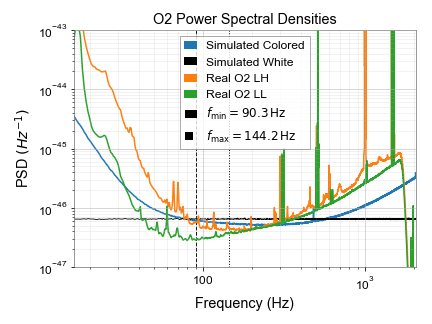
As evident from Table 2 and Figure 4, we find relatively good agreement (within %) of the recovered parameters of the CoCoA detection statistic on real data, simulated colored noise, and simulated white Gaussian noise (in both the absence and presence of a signal), with the analytical predictions described in Section II.

Ratio between analytical (Section II) and recovered values of the statistic for: simulated white Gaussian noise matched to LIGO S6, O1, and O2 sensitivities in the frequency range spanned by CM09long (Fig. 2, black); simulated colored Gaussian noise matched to S6, O1, and O2 sensitivities (Fig. 2, blue); real LIGO S6, O1, and O2 data (Fig. 2, orange and green). We note that in the matched-filter and semi-coherent limits the recovered number of d.o.f. is also consistent with the expectations of 2 and , respectively, within .
| Stochastic limit | |||
| PSD | |||
| (noise only) | (noise+signal) | (noise+signal) | |
| White S6 | 1.00 | 0.93 | 1.04 |
| Colored S6 | 0.98 | 0.92 | 0.98 |
| Real S6 | 0.90 | 0.96 | 0.98 |
| White O1 | 0.99 | 1.09 | 0.99 |
| Colored O1 | 1.03 | 1.13 | 0.99 |
| Real O1 | 1.08 | 1.09 | 0.99 |
| White O2 | 0.98 | 1.07 | 0.99 |
| Colored O2 | 1.01 | 1.11 | 1.02 |
| Real O2 | 1.05 | 1.09 | 1.02 |
| Matched-filter limit | |||
| PSD | |||
| (noise only) | (noise+signal) | (noise+signal) | |
| White S6 | 0.99 | 1.13 | 0.97 |
| Colored S6 | 0.98 | 1.00 | 1.06 |
| Real S6 | 0.97 | 0.95 | 1.02 |
| White O1 | 1.04 | 1.01 | 1.02 |
| Colored O1 | 0.95 | 1.06 | 0.98 |
| Real O1 | 1.11 | 0.96 | 0.94 |
| White O2 | 0.91 | 0.93 | 0.99 |
| Colored O2 | 1.00 | 1.00 | 1.02 |
| Real O2 | 1.04 | 0.96 | 1.02 |
| Semi-coherent approach () | |||
| PSD | |||
| (noise only) | (noise+signal) | (noise+signal) | |
| White S6 | 1.00 | 1.12 | 0.91 |
| Colored S6 | 1.12 | 0.97 | 1.09 |
| Real S6 | 1.02 | 0.84 | 1.10 |
| White O1 | 1.05 | 1.02 | 1.03 |
| Colored O1 | 1.09 | 1.02 | 1.03 |
| Real O1 | 1.04 | 1.09 | 0.97 |
| White O2 | 0.99 | 0.99 | 0.94 |
| Colored O2 | 1.00 | 1.06 | 1.01 |
| Real O2 | 1.02 | 0.90 | 1.03 |


V Multi-trial search for GRB remnants
In a realistic search for GWs from GRB remnants, the large uncertainties that affect the post-merger / post-explosion physics need to be taken into account. Even though CoCoA allows tuning of sensitivity/robustness so that some degree of uncertainty can be tolerated on the expected time-frequency track of the GW signal (see Section II), larger departures from such a track would cause the search to fail. In this Section we address the need for a large parameter space exploration, give an order-of-magnitude estimate for the implied computational cost of a search spanning such space, and describe the practical implementation of a multi-trial detection statistic for CoCoA.
V.1 Remnant properties and timing uncertainties
For the specific case of GWs from bar-mode instabilities of rotating magnetars discussed in Section III, a realistic search with CoCoA should be performed over a template bank spanning the possible range of parameters (, , , , ), where accounts for the uncertainty on the onset time of the secular bar-mode instability, something not considered in Coyne et al. 2016.
In Coyne et al. Coyne et al. 2016 we have shown that, for searches based on CM09long, the maximum errors one could tolerate on the assumed magnetar properties are of the order of M⊙, Gauss, km. With these errors, the sensitivity of a CoCoA semi-coherent search with optimized approaches that of a stochastic search on a perfectly matching template33 3 The last is also comparable to the maximum sensitivity of more robust and less computationally expensive algorithms that don’t rely on any prior knowledge of the signal time-frequency evolution (e.g. STAMP; see Abbott et al. 2017b)..
For GRBs observed on-axis and forming a long-lived, secularly unstable magnetar, the expected X-ray plateau duration and luminosity depend on the initial values of , , and , which can thus be constrained to some specific ranges by comparison with the observations Tang et al. 2019. Moreover, as demonstrated in the case of GW170817 Abbott et al. 2017b, for short GRBs some constraints on the remnant mass can be derived from the analysis of the pre-merger signal itself. The optimal case, of course, would be that of a short GRB with an observed X-ray plateau for which an in-spiral signal is also detected. In this case, joint electromagnetic and GW observations would enable us to set some constraints on all relevant parameters.
Regarding the uncertainty on , for long GRBs formed from collapsing massive stars we can reasonably assume that the delay between the collapse (and formation of the remnant) and that of the GRB trigger itself is of order 120 s Abbott et al. 2017a; Abadie et al. 2012. Thus, s (where is the GRB trigger time in -rays). In the case of short GRBs from merger of compact objects, the delay between the merger and the GRB trigger time is expected to be of the order of a few seconds, thus we assume s Abbott et al. 2017a; Abadie et al. 2012. The timing uncertainty on may be further reduced when or are more distinctly known through the detection of GWs produced by the merger/collapse. This was the case for GW170817, in which s Abbott et al. 2017b.
Motivated by the above considerations, in this analysis we vary between (where is 120 s for long GRBs and s for short GRBs) and , in steps of .
V.2 Computational cost: Order-of-magnitude estimate
As an order of magnitude estimate of the computational cost for a multi-trial CoCoA search that accounts for the uncertainties described in the previous Section, let us consider a post-merger search similar to that performed by (Abbott et al. 2017b) for GW170817. The last assumed fixed values of and , and large uncertainties in and (see also Bar1-Bar6 in Table 1). With a parameter space resolution of G and km for the magnetic field and NS radius, respectively, ranges of G and km, (see Section III for discussion of this range) could be spanned with a total of templates. With s and s we take 10 trials to cover the full timing uncertainty, making the total number of templates become (see Section VI.1).
A search with of requires running on order 2500 background realizations per template. This number of realizations ensures that the probability distribution above the threshold is populated with 25 events, thus resulting in an error of for the corresponding detection efficiency.
A CoCoA search on a single time-frequency track (as described in Section II) with of and 2500 background realizations is estimated to require core-hours or ‘‘Standard Units’’ (SUs44 4 An “SU” is an XSEDE Service Unit on Stampede, equal to 1 CPU core-hour on a 2.7 GHz E5-2680 Intel Xeon (Sandy Bridge) processor. E.g., a 1 hour allocation on a 8-core Stampede CPU would consume 8 SUs.). So a GRB search at on a template bank with time-frequency tracks would require MSUs. Assuming potentially nearby GRBs with X-ray plateaus and good LIGO Hanford/Livingston data in a 1 yr run, we estimate a full-run multi-trial GRB search to require MSUs, which is similar to the computational cost of other LIGO searches (e.g., Caride et al. 2019).
For a two-detector CoCoA search with a template bank similar to the GW170817 post-merger analysis described here, constructing 2500 independent background realizations per template requires d of coincident background data. This is comparable to e.g. what was used in Abbott et al. 2017b, where 5.6 d of background data were derived from non-continuous stretches of LL and LH coincident data from 2017 August 13-21 UT. We estimate that the SFTs of a d-long stretch of data will consume 80 GB of disk space per detector.
V.3 Multi-trial detection statistic
When uncertainties on the signal properties are large and searching over multiple time-frequency tracks (template bank) becomes necessary, the detection statistic of CoCoA needs to be modified to account for the larger number of trials. Hereafter, a CoCoA search on a single template in a bank (see Section II) will be referred to as a single trial.
To cover a given template bank, one performs a total of searches, each returning a certain value of the single-trial statistic defined as in Section II. In general, the probability distribution of changes across the template bank because it depends on the properties of the time-frequency tracks that constitute the bank itself. It is thus convenient to introduce a normalized statistic, which in the stochastic limit we define as
| (32) |
where is a Gaussian random variable calculated along the m-th template as in Eq. (16), with mean and standard deviation and given by Eqs. (17) and (18), respectively. In the matched filter limit, we define the normalized statistic as:
| (33) |
where and are calculated along the m-th template as in Eqs. (21) and (22), respectively, with a random variable distributed as a with two degrees of freedom and with non-centrality parameter given by Eq. (25). Finally, in the semi-coherent approach we set:
| (34) |
where and are calculated along the -th template as in Eqs. (21) and Eq. (26), respectively, with a random variable distributed as a with degrees of freedom, and non-centrality parameter given by Eq. (25). In the above definition, we also assume that the same is adopted (and optimized) across trials (see Section VI).
With the above normalization, we define the maximum statistic as =max for , which we use to identify the most statistically promising detection candidates. Generally speaking, in the presence of a signal, we expect the template that is most similar to the signal to return the maximum value of the statistic. For a given choice of , we thus set the corresponding detection threshold as:
| (35) |
where is the probability that any of the templates in the bank (trial) returns the largest value . For completely independent trials, this probability reads:
| (36) |
where is the probability distribution of .
In the absence of a signal, the probability distribution of the normalized statistic is the same for all trials, thus for all and above Equation simplifies to Abadie et al. 2010:
| (37) |
Integrating both sides of the above Equation, and considering Eq. (35), we get:
| (38) |
If the FAP is small, then for and we can approximate Eq. (38) as:
| (39) |
The above approximation is useful as it shows that the threshold of a multi-trial search can be estimated analytically from the threshold of a single trial search. We finally note that for searches where the individual trials are not fully independent, the probability of a given is generally lower than what is predicted in Equation (36), so one can define an effective number of trials . In the case of GRB magnetars, templates are fully independent only when their time-frequency tracks as determined by (, , , , ) do not intersect.
VI CoCoA multi-trial search tests
As discussed in Section V, in a post-GRB search for GWs from secularly unstable magnetars, it is necessary to build a multi-trial search that accounts not only for the uncertainties on the magnetar properties (, , , ), but also for the uncertainty that affects the timing between the GRB trigger time as established by -ray observations, and the onset of the bar-mode instability. Hereafter, we present the results of tests aimed at verifying the agreement between the analytical expectations for the CoCoA multi-trial statistic described in Section V and the actual code performance on simulated data, as well as demonstrating the sensitivity of a CoCoA search. Our tests proceed as follows:
- 1.
We simulate colored Gaussian noise with PSD matching that of LIGO O2, sampled at kHz. We assume two detectors with identical PSDs, use s, and set =1% for determining our detection threshold (see Eq. (35)).
- 2.
We simulate a region of data extending between and , where is an arbitrary GRB trigger time, is the timing uncertainty between the collapse/merger and the GRB trigger time and is the duration of the waveform being searched for. We take two values for , 120 s to simulate a standard long GRB and 2 s to simulate an event similar to GW170817 (see Section V.2).
- 3.
We assume a known GRB sky location and set and for LIGO Hanford, and and for LIGO Livingston (comparable to those of GW170817 Abbott et al. 2017; Abbott et al. 2017b).
- 4.
When constructing a template bank for the search we vary in the range (see Section V.1) for each choice of . We sample this range in steps that are multiples of i.e., . The choice of is made with computational cost in mind given that the smaller , the larger the number / of templates required to account for the timing uncertainty.
- 5.
To estimate our detection efficiency, we inject signals in the simulated O2 data assuming we are aligned with the GRB jet axis (i.e., in Eqs. (7)-(8)), as expected for GRBs with X-ray plateaus. The injection time is set to always fall exactly in between the onset times of two randomly chosen, temporally adjacent templates in the bank, i.e. . With this choice, we maximize the temporal mismatch between the injected signal and the closest template in the bank, thus obtaining a conservative estimate of CoCoA’s detection efficiency.
- 6.
Similarly to what is done in Coyne et al. 2016, for each waveform we calculate the detection efficiency as a function of luminosity distance, and derive a distance horizon by requiring a false dismissal probability (see Figure 10).
VI.1 Timing uncertainties
In order to first isolate the effects of timing uncertainties only, here we carry out a multi-trial CoCoA search where the signal we search for is assumed to be produced by a magnetar with exactly known parameters (, , , ), but with unknown onset time . We thus define a template bank composed of CM09long-like/CM09short-like waveforms (see Section III) whose onset time is varied as described in the previous Section.
VI.1.1 Background statistic


As shown in Figure 5, in the absence of a signal, the recovered multi-trial background statistic (grey histogram) for various choices of and can show deviations from the analytical expectations described in Section V.3 (black dashed line; see also Eq. (37)). Those expectations assumed that trials are completely independent (see Eq. (37)), which is not always the case. Indeed, varying the onset times of otherwise identical time-frequency tracks can introduce dependencies between trials, which in turn imply that the recovered background distribution is equivalent to a predicted background distribution with an effective number of trials that is lower than the one obtained assuming that all templates in the bank are independent.
Dependencies among templates become more important for smaller values of , as evident by comparing the top-left and top-right panels of Figure 5. The recovered probability distribution (grey histogram) agrees well with the predictions discussed in Section V.3 (black-dashed line) for large (top-left panel). However, for smaller in an otherwise identical search (top-right), the recovered results deviate from the expected ones.
To describe the actual recovered background statistic for a non-fully independent template bank, we thus introduce an effective number of trials determined as described in Appendix A. The red-dashed lines in Figure 5 show that this effective background distribution agrees well with the recovered one (histogram; note that in the top-left panel the black- and red-dashed lines overlap completely).
Other factors affecting the effective number of trials include the rate at which the considered waveform evolves. For example, in a search for the faster evolving waveform CM09short, the time-frequency tracks of different trials in the bank are less likely to have significant overlaps (and thus related trial dependencies) even for small values of (bottom-right panel in Figure 5). Finally, smaller values of result in a larger degree of statistical dependence between templates (compare the top-left and bottom-left panels in Figure 5). Indeed, for a given number of overlapping time-frequency bins between two templates in a bank, the smaller the coherence time, the larger the fraction of dependent pairs (i.e. pairs generated from cross-correlation products containing time-frequency bins in the overlapping portion of the templates time-frequency track) to the total number of pairs entering in the computation of along each template. Incidentally we note that, conceptually, this effect is similar to what is behind the larger robustness of semi-coherent searches with smaller coherence timescales: if only a few time-frequency bins overlap between the injected signal and the closest template in a bank, smaller coherence times imply that cross-correlation products from these few overlapping bins have a larger relative weight in the computation of along the template.
VI.1.2 Detection efficiency and search sensitivity
= 120 s


= 120 s


= 2 s


Our goal with CoCoA is to use its tunability so that we can maximize detection efficiency and ensure that the achieved distance horizon for a semi-coherent multi-trial search is always larger than even the most sensitive stochastic (and thus less computationally expensive) search, i.e. a single-trial stochastic search with a template perfectly matching the injected waveform. This justifies the use of CoCoA over less computationally demanding stochastic algorithms Thrane et al. 2011; Thrane and Coughlin 2013; Thrane and Coughlin 2014; Thrane et al. 2015; Coughlin et al. 2011; Abbott et al. 2017b. In what follows, we demonstrate that we can reach this goal in a multi-trial CoCoA search accounting for timing uncertainties.
In Figures 6-8 we quantify the sensitivity of a CoCoA search incorporating timing uncertainties in the presence of CM09long/CM09short signals for a source located at the GW170817 position (see Section VI). Specifically, in the various panels of Figures 6-8 we show the distance horizon corresponding to a of 50% as a function of the coherence time of the search, for the CM09long/CM09short waveforms with different values of timing uncertainties, s.
Unsurprisingly, the best sensitivities (largest distance horizons) are achieved when is equal to a single SFT baseline (as this implies minimizing the difference between the injected waveform and the closest template in the bank). Note also that the smaller the , the larger the optimal coherence time of the search. This is to be expected as larger coherent times improve sensitivity at the expense of robustness against signal uncertainties. Thus, we can afford larger coherence times for smaller differences between the closest template in our bank and the injected waveform, i.e. for smaller . These Figures also show that a coarser choice of reduces the computational cost of the search, as larger correspond to smaller . This occurs at the expense of sensitivity: indeed, for , the CoCoA distance horizon with optimized coherence time approaches the stochastic-like horizon (blue-dashed line). On the other hand, smaller greatly improve sensitivity but imply larger number of trials and increased computational cost. To make a concrete example, the distance horizon we achieve for a search on CM09long with 120 s of timing uncertainty and in O2-like data is Mpc (top-left panel in Figure 6). However, such a search would require nearly 500 individual trials just to account for the timing uncertainty, and it would quickly become prohibitively costly computationally if one were to also account for uncertainties in the magnetar physical parameters (see Section V.2). Thus, a more realistic search for CM09long and s would be one with , as this produces 9 trials, which can be handled computationally even when uncertainties on the magnetar physical parameters are considered (see Section V.2). We note that an CoCoA search with timing uncertainties produces a distance horizon of Mpc. The last, rescaled for an optimally located source and for advanced LIGO nominal sensitivity (as in Abbott et al. 2018a), corresponds to Mpc (only slightly less than the actual distance of GW170817).
If the timing uncertainty can be reduced to s (see Section V.1), as was the case for GW170817, then a search with produces only 9 trials, and would be computationally accessible even considering uncertainties on the post-GRB magnetar properties (see discussion in Section V.2). We stress that the horizon distance of a search with s and is Mpc (see Figure 8), or Mpc for an optimally oriented source and for advanced LIGO nominal sensitivity. We note that this is comparable to the sensitivity of a single-trial search of CM09long with advanced LIGO nominal sensitivity and the same choices of and , which produces a distance horizon of 63 Mpc with a of 1.
Finally, as shown in Figure 7, faster evolving waveforms (such as CM09short) with large timing uncertainties ( s) are more effectively searched for with a stochastic-like algorithm rather than with a semi-coherent CoCoA approach as the last produces horizon distances smaller than the stochastic-like horizon (blue-dashed lines) for . However, as evident from Figure 8, when the timing uncertainty can be reduced s (as for GW170817), CoCoA can achieve large distance horizons ( Mpc) for a very reasonable number of trials. This implies that a search for a CM09short waveform for an optimally oriented source with advanced LIGO at nominal sensitivity could reach distances of order 100 Mpc. We note that this is comparable to the sensitivity of a single-trial search of CM09short with advanced LIGO nominal sensitivity and the same choices of and , which produces a distance horizon of 140 Mpc with a of 1.
VI.2 Uncertainties in both timing and magnetar properties
In this Section we follow an approach similar to what is described in the previous one to quantify the CoCoA sensitivity and detection efficiency in the presence of both timing uncertainties and uncertainties in the physical parameters of the GRB remnant (see Section V.1). Namely, we inject CM09long/CM09short in simulated data with sensitivity matched to LIGO O2, and run a search using a template bank that accounts for both and uncertainties on (, , , ). The last are taken into account by constructing a template bank where waveforms corresponding to steps of sizes G, km, around the values of CM09long/CM09short are used (see also Coyne et al. 2016). All combinations of shifts to , , and are included in our template bank, giving a total of 26 unique time-frequency tracks per each of the CM09long and CM09short waveforms. We note that we do not include the exact injected waveform in our template bank so as to derive a conservative estimate of the detection efficiency.


In Figure 9 (left) we show the results of a search for CM09long with and s, which produces 9 trials accounting for timing uncertainties per each of the 26 possible choices of steps in , , and accounting for uncertainties in these parameters. This yields a total of 234 trials. As evident by comparing the results in Figure 9 (left panel) with those shown in the center-right panel of Figure 6, in spite of the increased number of trials, when all possible uncertainties are considered overall the template in the bank closest to the injected waveform has a smaller mismatch than it would have by only considering timing uncertainties. In other words, small shifts in magnetar parameter values can compensate the mismatch introduced by timing uncertainties.
Similar results are found for a search of the CM09short waveform, with s, (compare the right panel in Figure 9 to the right panel in Figure 8). In this case we find that for a fast-evolving waveform such as CM09short, small shifts in magnetar parameters combined with small shifts in the start time of GW emission may still compensate eachother, potential error of the onset time of GW emission is smaller than a single SFT. This is a surprising, yet welcome result as this compensation provides an even higher degree of sensitivity to our search. Indeed, this result provides a distance horizon of 51.3 0.7 Mpc, which scales above 110 Mpc for an optimally oriented source with advanced LIGO nominal sensitivity.

VII Summary and conclusion
In this work we have demonstrated the potential that CoCoA has for realistic targeted searches of GW signals of durations ranging from a few hundred to a few thousand seconds. Results have been shown specifically for the case of bar-mode instabilities of millisecond magnetars formed in GRBs Corsi and Mészáros 2009, but can be easily generalized to other time-frequency tracks of similar durations associated with quasi-monochromatic GW signals.
Compared to the results originally presented in Coyne et al. 2016, we have further developed CoCoA to ensure it can run on real GW detectors data, and that it can incorporate a multi-trial statistic allowing for searches spanning a bank of templates accounting for signal uncertainties. We have also provided order-of-magnitude estimates for the computational cost associated with various types of CoCoA searches.
Overall our results are encouraging, as the expected distance horizons for CoCoA searches on an optimally oriented source are comparable to, or exceed, the distance of GW170817 when assuming advanced LIGO nominal sensitivity. For a binary NS merger rate in the range (0.32 - 4.760) Mpc-3 yr-1 Abbott et al. 2018b; Abbott et al. 2017, we expect 0.1 - 1 events yr-1 within 40 Mpc, and 1 - 20 events yr-1 within 100 Mpc (which should be within CoCoA reach once advanced LIGO reaches nominal sensitivity, as demonstrated here). Of these, based on current limited estimates of short GRBs opening angles (e.g., (Fong et al. 2012)), would launch jets aligned with our line of sight and could thus show X-ray plateaus which would enable us to set even more stringent constraints on a potential magnetar remnant. Thus, a targeted CoCoA search for short GRB remnants that employs a full parameter space at full advanced detectors’ sensitivity may be capable of either making detections, or else significantly constraining the most optimistic theoretical models.
In terms of sensitivity, our results improve substantially on the ones previously presented e.g. in Abbott et al. 2017b, but require stricter conditions on the timing uncertainties so as to ensure that a template-based CoCoA search is computationally feasible. In Appendix B we discuss in more details how the CoCoA results presented here complement past searches such as the ones in Abbott et al. 2017b.
We finally note that magnetars may also be formed in long-duration GRBs. Thus, long GRBs (and specifically those with the characteristic X-ray plateau), will also provide interesting targets for CoCoA. Long-duration GRBs are estimated to have observed rates in the range 0.7-103 Gpc-3 yr-1 (depending on luminosity; see e.g. (Liang and Zhang 2006; Virgili et al. 2009; Sun et al. 2015)). Using the nominal advanced LIGO horizon distance for a CoCoA search of CM09long of (30 Mpc; see Section VI.1), we can expect events yr-1. Thus, targeted searches for magnetars formed in long GRBs will likely need to wait for second or third generation ground-based detectors Daw a; Daw b; Miller et al. 2015. For example, the recently funded upgrade for advanced LIGO envisions an increase in the volume of space the observatory can survey by as much as seven times Daw a, which would make long GRB searches with CoCoA come into reach on more reasonable timescales.
Appendix A Effective number of trials and detection efficiency error estimation
In Section VI.1 and Figure 5 we discuss results of the CoCoA background distribution from multi-trial tests. These results show a difference in the expected probability distribution (as in Eq. (37)) and the recovered distribution. This difference is caused by overlapping time-frequency tracks of different templates in the template bank, and is quantified in Figure 5 via the definition of an effective number of trials. The method we use to calculate the effective number of trials is defined below.
We start by solving Equation (37) for many different probability distribution functions (P()) using values of effective trials () ranging from 0.1 to the true + 1 with steps of 0.1 trials. After generating the probability function in Equation (37) for each sampled value of we take the integral of the probability function to generate the cumulative distribution function (CDF55 5 Integration performed using the python scipy integration tool cumtrapz, which uses cumulative trapezoidal integration technique. For more information see httpsdocs.scipy.org/doc/scipy/reference/tutorial/integrate.html Jones et al. 2001– ). The CDF for each value of is then compared to the empirical cumulative distribution function (ECDF66 6 ECDFs are calculated using the python library statsmodels’ ECDF function in the distributions sub-library. For more information see https Josef Perktold 2009–.) from the recovered results. The comparison is done by using the coefficient of determination () which is defined by:
| (40) |
where refers to observed data, refers to the mean of observed data and refers to expected data Barrett 1974. In our case refers to the ECDF from recovered results and refers to the analytic CDF generated from a given value of . The that produces an value closest to 1 is taken as the chosen value of .
The error on the effective number of trials is calculated considering that an ECDF has an error bound by the Dvoretzky-Kiefer-Wolowitz (DKW) inequality Wei and Dudley 2011; Dvoretzky et al. 1956. The DKW inequality is a concentration inequality which provides bounds on how a variable deviates from its expected value. Specifically, the error on the ECDF (such that the true ECDF lies between the recovered ECDF + and the recovered ECDF - ), is defined as:
| (41) |
where is the associated probability, is the number of samples (in our case the number of background realizations as in Section V.2). To estimate the error on we thus perform tests similarly to what described above, but using the ECDF . The difference between the found when performing the test on the ECDF and those found when performing the same test on the ECDF is taken as the error in . As the test only considers discretely sampled values of , 0.1 effective trials apart, we also add an additional systematic error of 0.05 on the estimated .
The DKW inequality is also used in the calculation of errors on the detection efficiency and distance horizons. Because the threshold for a given search makes use of the ECDF, the in Equation (41) also puts bounds on our error on the detection efficiency for a chosen (red errors bars in Figure 10). The recovered efficiencies at each injected distance, as well as their upper- and lower-error ranges are then fit to sygmoid curves (see the dashed lines in Figure 10). The distance that corresponds to the point where the chosen level (black-dotted line in Figure 10) crosses the sigmoid fit to the detection efficiency (black-dashed line in Figure 10), is then taken as the distance horizon for that given (marked in green in Figure 10). The error on such distance is estimated by using the points where the sygmoids fits to the upper and lower bounds of the efficiency curve (red-dashed lines in Figure 10) cross the chosen (black-dotted line in Figure 10).
Appendix B Order-of-magnitude comparison with previous GW170817 post-merger results
Searches for post-merger GWs from secularly unstable magnetars with parameters matched to those of Bar1-Bar6 (see Section III) have been performed for GW170817 using the Stochastic Analysis Multi-detector Pipeline (STAMP) Coughlin et al. 2011; Thrane and Coughlin 2013; Abbott et al. 2017b. STAMP searches for excess power in time-frequency maps by cross-correlating data streams of different detectors and using pattern recognition algorithms rather than a template bank of time-frequency tracks. For the pattern recognition, STAMP uses both seed-based (Zebraguard) and seedless (Lonetrack) algorithms. Because STAMP searches are most similar to the CoCoA stochastic limit, here we compare expectations for a stochastic-limit CoCoA search on Bar1-Bar6 with STAMP results on these same waveforms reported in Abbott et al. 2017b.
We consider a CoCoA search similar to that described in Section VI, with s, and and matching those used for the STAMP search in Abbott et al. 2017b. An appropriate template bank for such as CoCoA search would include waveforms Bar1-6, as well as a range of other waveforms with same and but spanning ranges of km for the NS radius, and G for the magnetic field, in steps of G and km (see Section VI.2). For this choice in step size the CoCoA template bank would contain 100 templates to span the possible values of , and 490 templates to span the possible values of . Temporal uncertainty can be accounted for by choosing s, which is comparable to the delay between the merger time of GW170817 and its associated GRB 170817A (see Sections V.2 and VI.1 for more discussion). With s (as in Section VI), this would result in 9 choices of for each (, , , ). Thus, we expect a CoCoA search to include trials.
In order to estimate the sensitivity of a CoCoA search without spending a large amount of computational time, we compute our background statistic using a reduced template bank that only considers Bar1-6 and all combinations of physical parameters that are one step away from Bar1-6. The background is built using 9.1 days of coincident detector data during the O2 LIGO run, starting 20 days before the GW170817 merger and ending 1 hour before. The results are displayed in Figure 11. From the grey histogram in this Figure we calculate the corresponding to a and find this to be in excellent agreement with what expected from simulated Gaussian noise with O2-like sensitivity (pink histogram in Fig. 11). Next, we use Eq. (39) to estimate the of a search with (see above) and . We then estimate the CoCoA distance horizon for Bar1-Bar6 by injecting those signals in the longest O2 stretch of data closest to the trigger time of GW170817 (starting at GPS time 1186898000), and searching with a template bank that considers all combinations of physical parameters one step away from the injected waveform (this is similar to what is done in Section VI.2). The results of this test are compared to STAMP’s results for GW170817 in Figure 12.


From Figure 12 we see that CoCoA (blue bars), even in its least sensitive stochastic limit, is more sensitive than STAMP. But, the gained sensitivity comes at the expenses of computational cost. This is ultimately related to the fact that while CoCoA is a template-based search that considers the expected physics behind the time-frequency tracks it searches for, STAMP time-frequency maps are build using analytic methods that do not consider specific models. While this reduces the STAMP search sensitivity, it makes it computationally more feasible in the presence of large signal uncertainties. Indeed, the red and green bars in Figure 12 show the results of the STAMP search reported in Abbott et al. 2017b. The last targeted bar-like GWs starting at the time of the GW170817 merger and ending 8.5 days after the merger, thus allowing for a much greater than the 2 s considered for a CoCoA search (light and dark blue bars). The STAMP search was carried out using time-frequency maps of duration 500 s, times with 50 overlap from the previous time-frequency map, and an SFT duration of 1 s, for a total of trials. If we were to build a CoCoA search with the same choice of days and keeping s, we would need choices of for each (, , , ) and trials for the full search (Fig. 12, light blue). A search of this magnitude would cost 250 GSUs, which is 5 orders of magnitude larger than other LIGO searches, (e.g., Caride et al. 2019) and is therefore computationally unfeasible.
In conclusion, we can say that the STAMP and CoCoA approaches are complementary, and we advocate for running searches with both as the most likely way for maximizing chances of detecting intermediate-duration post-merger signals.
Appendix C Additional Tests
In this Section we show how the performance of CoCoA changes by changing some of the assumptions we made in Section VI.1. Specifically, we consider (i) changing the from 50% to 10%; and (ii) randomizing the injection time rather than having it always fall exactly in between two adjacent SFT bins (a choice that maximizes the mismatch between injections and templates). We test these changes on two representative searches. A first search of CM09long with s, , and s; and a second search of CM09short with s, , and and s. These coherence time values are chosen based on the optimization procedure shown in Figures 6 and 8.
Our results are reported in Table 3, where for reference we also show the distance horizons obtained for , for injections times matching exactly the start times of the template waveforms (which eliminates the mismatch between the two; see and in Table 3), and for injection times always in between adjacent SFT bins (which maximizes the mismatch between injected and template waveforms; see and in Table 3).
| Waveform | |||||||||
|---|---|---|---|---|---|---|---|---|---|
| (s) | (s) | (Mpc) | (Mpc) | (Mpc) | (Mpc) | (Mpc) | (Mpc) | ||
| CM09long | 1 | 120 | 60 | 15.0 0.5 | 12.3 0.4 | 12.8 0.5 | 10.4 0.4 | 13.6 0.5 | 11.5 0.4 |
| CM09short | 4 | 2 | 1 | 60.0 0.7 | 46.0 0.7 | 45.5 0.7 | 37.9 0.6 | 52.8 0.7 | 42.6 0.6 |
Unsurprisingly, when the onset time is randomized, the sensitivity of the search (see and in Table 3) falls in between the two extremes of no mismatch and maximized mismatch. Also unsurprisingly, we find that decreasing the allowed reduces the sensitivity of the search, so the distance horizons for are smaller than for .
Acknowledgements.
This work is supported by the National Science Foundation via CAREER award #1455090 (PI: Alessandra Corsi). We thank Benjamin J. Owen for general discussions on topics related to this work. This paper has document number LIGO-P1500226.References
- Kouveliotou et al. (1993) C. Kouveliotou, C. A. Meegan, G. J. Fishman, N. P. Bhat, M. S. Briggs, T. M. Koshut, W. S. Paciesas, and G. N. Pendleton, Identification of two classes of gamma-ray bursts, Astrophys. J. Lett. 413, L101 (1993).
- Woosley (1993) S. E. Woosley, Gamma-ray bursts from stellar mass accretion disks around black holes, Astrophys. J. 405, 273 (1993).
- Popham et al. (1999) R. Popham, S. E. Woosley, and C. Fryer, Hyperaccreting Black Holes and Gamma-Ray Bursts, Astrophys. J. 518, 356 (1999), eprint astro-ph/9807028.
- Piran (1999) T. Piran, Gamma-ray bursts and the fireball model, Physics Reports 314, 575 (1999), eprint astro-ph/9810256.
- Lei et al. (2013) W.-H. Lei, B. Zhang, and E.-W. Liang, Hyperaccreting Black Hole as Gamma-Ray Burst Central Engine. I. Baryon Loading in Gamma-Ray Burst Jets, Astrophys. J. 765, 125 (2013), eprint 1209.4427.
- Lei et al. (2017) W.-H. Lei, B. Zhang, X.-F. Wu, and E.-W. Liang, Hyperaccreting Black Hole as Gamma-Ray Burst Central Engine. II. Temporal Evolution of the Central Engine Parameters during the Prompt and Afterglow Phases, Astrophys. J. 849, 47 (2017), eprint 1708.05043.
- Dainotti and Del Vecchio (2017) M. G. Dainotti and R. Del Vecchio, Gamma Ray Burst afterglow and prompt-afterglow relations: An overview, New Astronomy Reviews 77, 23 (2017), eprint 1703.06876.
- Kisaka et al. (2017) S. Kisaka, K. Ioka, and T. Sakamoto, Bimodal Long-lasting Components in Short Gamma-Ray Bursts: Promising Electromagnetic Counterparts to Neutron Star Binary Mergers, Astrophys. J. 846, 142 (2017), eprint 1707.00675.
- Nousek et al. (2006) J. A. Nousek, C. Kouveliotou, D. Grupe, K. L. Page, J. Granot, E. Ramirez-Ruiz, S. K. Patel, D. N. Burrows, V. Mangano, S. Barthelmy, et al., Evidence for a Canonical Gamma-Ray Burst Afterglow Light Curve in the Swift XRT Data, Astrophys. J. 642, 389 (2006), eprint arXiv:astro-ph/0508332.
- Zhang et al. (2006) B. Zhang, Y. Z. Fan, J. Dyks, S. Kobayashi, P. Mészáros, D. N. Burrows, J. A. Nousek, and N. Gehrels, Physical Processes Shaping Gamma-Ray Burst X-Ray Afterglow Light Curves: Theoretical Implications from the Swift X-Ray Telescope Observations, Astrophys. J. 642, 354 (2006), eprint arXiv:astro-ph/0508321.
- Liang and Zhang (2006) E. Liang and B. Zhang, Calibration of gamma-ray burst luminosity indicators, Mon. Not. R. Astron. Soc. 369, L37 (2006), eprint astro-ph/0512177.
- Starling et al. (2008) R. L. C. Starling, P. T. O’Brien, R. Willingale, K. L. Page, J. P. Osborne, M. de Pasquale, Y. E. Nakagawa, N. P. M. Kuin, K. Onda, J. P. Norris, et al., Swift captures the spectrally evolving prompt emission of GRB070616, Mon. Not. R. Astron. Soc. 384, 504 (2008), eprint 0711.3753.
- Bernardini et al. (2012) M. G. Bernardini, R. Margutti, J. Mao, E. Zaninoni, and G. Chincarini, The X-ray light curve of gamma-ray bursts: clues to the central engine, Astron. Astrophys. 539, A3 (2012), eprint 1112.1058.
- Gompertz et al. (2013) B. P. Gompertz, P. T. O’Brien, G. A. Wynn, and A. Rowlinson, Can magnetar spin-down power extended emission in some short GRBs?, Mon. Not. R. Astron. Soc. 431, 1745 (2013), eprint 1302.3643.
- Rowlinson et al. (2013) A. Rowlinson, P. T. O’Brien, B. D. Metzger, N. R. Tanvir, and A. J. Levan, Signatures of magnetar central engines in short GRB light curves, Mon. Not. R. Astron. Soc. 430, 1061 (2013), eprint 1301.0629.
- Yi et al. (2014) S. X. Yi, Z. G. Dai, X. F. Wu, and F. Y. Wang, X-Ray Afterglow Plateaus of Long Gamma-Ray Bursts: Further Evidence for Millisecond Magnetars, ArXiv e-prints (2014), eprint 1401.1601.
- Ravi and Lasky (2014) V. Ravi and P. D. Lasky, The birth of black holes: neutron star collapse times, gamma-ray bursts and fast radio bursts, Mon. Not. R. Astron. Soc. 441, 2433 (2014), eprint 1403.6327.
- Yu et al. (2017) Y.-W. Yu, L.-D. Liu, and Z.-G. Dai, A long-lived remnant neutron star after GW170817 inferred from its associated kilonova, ArXiv e-prints (2017), eprint 1711.01898.
- Abbott et al. (2017a) B. P. Abbott, R. Abbott, T. D. Abbott, F. Acernese, K. Ackley, C. Adams, T. Adams, P. Addesso, R. X. Adhikari, V. B. Adya, et al., GW170817: Observation of Gravitational Waves from a Binary Neutron Star Inspiral, Physical Review Letters 119, 161101 (2017a), eprint 1710.05832.
- Abbott et al. (2017b) B. P. Abbott, R. Abbott, T. D. Abbott, F. Acernese, K. Ackley, C. Adams, T. Adams, P. Addesso, R. X. Adhikari, V. B. Adya, et al., Search for Post-merger Gravitational Waves from the Remnant of the Binary Neutron Star Merger GW170817, Astrophys. J. Lett. 851, L16 (2017b), eprint 1710.09320.
- Abbott et al. (2019) B. P. Abbott, R. Abbott, T. D. Abbott, F. Acernese, K. Ackley, C. Adams, T. Adams, P. Addesso, R. X. Adhikari, V. B. Adya, et al., Search for Gravitational Waves from a Long-lived Remnant of the Binary Neutron Star Merger GW170817, Astrophys. J. 875, 160 (2019), eprint 1810.02581.
- Bonazzola and Gourgoulhon (1996) S. Bonazzola and E. Gourgoulhon, Gravitational waves from pulsars: emission by the magnetic-field-induced distortion., Astronomy and Astrophysics 312, 675 (1996), eprint astro-ph/9602107.
- Palomba (2001) C. Palomba, Gravitational radiation from young magnetars: Preliminary results, Astronomy and Astrophysics 367, 525 (2001).
- Cutler (2002) C. Cutler, Gravitational waves from neutron stars with large toroidal B fields, Phys. Rev. D 66, 084025 (2002), eprint gr-qc/0206051.
- Lai and Shapiro (1995) D. Lai and S. L. Shapiro, Gravitational radiation from rapidly rotating nascent neutron stars, Astrophys. J. 442, 259 (1995), eprint arXiv:astro-ph/9408053.
- Corsi and Mészáros (2009) A. Corsi and P. Mészáros, Gamma-ray Burst Afterglow Plateaus and Gravitational Waves: Multi-messenger Signature of a Millisecond Magnetar?, Astrophys. J. 702, 1171 (2009), eprint 0907.2290.
- Owen et al. (1998) B. J. Owen, L. Lindblom, C. Cutler, B. F. Schutz, A. Vecchio, and N. Andersson, Gravitational waves from hot young rapidly rotating neutron stars, Phys. Rev. D 58, 084020 (1998), eprint gr-qc/9804044.
- Lindblom et al. (1998) L. Lindblom, B. J. Owen, and S. M. Morsink, Gravitational Radiation Instability in Hot Young Neutron Stars, Physical Review Letters 80, 4843 (1998), eprint gr-qc/9803053.
- Andersson (1998) N. Andersson, A New Class of Unstable Modes of Rotating Relativistic Stars, Astrophys. J. 502, 708 (1998), eprint gr-qc/9706075.
- Zhang and Mészáros (2001) B. Zhang and P. Mészáros, Gamma-Ray Burst Afterglow with Continuous Energy Injection: Signature of a Highly Magnetized Millisecond Pulsar, Astrophys. J. Lett. 552, L35 (2001), eprint arXiv:astro-ph/0011133.
- Coyne et al. (2016) R. Coyne, A. Corsi, and B. J. Owen, Cross-correlation method for intermediate-duration gravitational wave searches associated with gamma-ray bursts, Phys. Rev. D 93, 104059 (2016), eprint 1512.01301.
- Thrane et al. (2011) E. Thrane, S. Kandhasamy, C. D. Ott, W. G. Anderson, N. L. Christensen, M. W. Coughlin, S. Dorsher, S. Giampanis, V. Mandic, A. Mytidis, et al., Long gravitational-wave transients and associated detection strategies for a network of terrestrial interferometers, Phys. Rev. D 83, 083004 (2011), eprint 1012.2150.
- The LIGO Scientific Collaboration et al. (2019) The LIGO Scientific Collaboration, the Virgo Collaboration, B. P. Abbott, R. Abbott, T. D. Abbott, S. Abraham, F. Acernese, K. Ackley, C. Adams, R. X. Adhikari, et al., All-sky search for long-duration gravitational-wave transients in the second Advanced LIGO observing run, arXiv e-prints (2019), eprint 1903.12015.
- Sun and Melatos (2018) L. Sun and A. Melatos, Application of hidden Markov model tracking to the search for long-duration transient gravitational waves from the remnant of the binary neutron star merger GW170817, arXiv e-prints (2018), eprint 1810.03577.
- Miller et al. (2018) A. Miller, P. Astone, S. D’Antonio, S. Frasca, G. Intini, I. La Rosa, P. Leaci, S. Mastrogiovanni, F. Muciaccia, C. Palomba, et al., Method to search for long duration gravitational wave transients from isolated neutron stars using the generalized frequency-Hough transform, Phys. Rev. D 98, 102004 (2018), eprint 1810.09784.
- Klimenko et al. (2016) S. Klimenko, G. Vedovato, M. Drago, F. Salemi, V. Tiwari, G. A. Prodi, C. Lazzaro, K. Ackley, S. Tiwari, C. F. Da Silva, et al., Method for detection and reconstruction of gravitational wave transients with networks of advanced detectors, Phys. Rev. D 93, 042004 (2016), eprint 1511.05999.
- Oliver et al. (2019) M. Oliver, D. Keitel, and A. M. Sintes, The Adaptive Transient Hough method for long-duration gravitational wave transients, Phys. Rev. D99, 104067 (2019), eprint 1901.01820.
- Blair (1991) D. G. Blair, The Detection of Gravitational Waves (1991).
- Jaranowski et al. (1998) P. Jaranowski, A. Królak, and B. F. Schutz, Data analysis of gravitational-wave signals from spinning neutron stars: The signal and its detection, Phys. Rev. D 58, 063001 (1998), eprint arXiv:gr-qc/9804014.
- Hinder et al. (2013) I. Hinder, A. Buonanno, M. Boyle, Z. B. Etienne, J. Healy, N. K. Johnson-McDaniel, A. Nagar, H. Nakano, Y. Pan, H. P. Pfeiffer, et al., Error-analysis and comparison to analytical models of numerical waveforms produced by the NRAR Collaboration, Classical and Quantum Gravity 31, 025012 (2013), eprint 1307.5307.
- Apostolatos (1995) T. A. Apostolatos, Search templates for gravitational waves from precessing, inspiraling binaries, Phys. Rev. D 52, 605 (1995), URL http://link.aps.org/doi/10.1103/PhysRevD.52.605.
- Sampson et al. (2014) L. Sampson, N. Cornish, and N. Yunes, Mismodeling in gravitational-wave astronomy: The trouble with templates, Phys. Rev. D 89, 064037 (2014), eprint 1311.4898.
- Brady and Creighton (2000) P. R. Brady and T. Creighton, Searching for periodic sources with LIGO. II. Hierarchical searches, Phys. Rev. D 61, 082001 (2000), eprint arXiv:gr-qc/9812014.
- Allen (2005) B. Allen, 2 time-frequency discriminator for gravitational wave detection, Phys. Rev. D 71, 062001 (2005), eprint arXiv:gr-qc/0405045.
- Cutler et al. (2005) C. Cutler, I. Gholami, and B. Krishnan, Improved stack-slide searches for gravitational-wave pulsars, Phys. Rev. D 72, 042004 (2005), eprint arXiv:gr-qc/0505082.
- Abbott et al. (2007) B. Abbott, R. Abbott, R. Adhikari, J. Agresti, P. Ajith, B. Allen, R. Amin, S. B. Anderson, W. G. Anderson, M. Arain, et al., Upper limit map of a background of gravitational waves, Phys. Rev. D 76, 082003 (2007), eprint arXiv:astro-ph/0703234.
- Abbott et al. (2009) B. P. Abbott, R. Abbott, F. Acernese, R. Adhikari, P. Ajith, B. Allen, G. Allen, M. Alshourbagy, R. S. Amin, S. B. Anderson, et al., An upper limit on the stochastic gravitational-wave background of cosmological origin, Nature (London) 460, 990 (2009), eprint 0910.5772.
- Coughlin et al. (2011) M. W. Coughlin, LIGO Scientific Collaboration, and Virgo Collaboration, Identification of long-duration noise transients in LIGO and Virgo, Class. Quant. Grav. 28, 235008 (2011), eprint 1108.1521.
- The LIGO Scientific Collaboration et al. (2014) The LIGO Scientific Collaboration, the Virgo Collaboration, J. Aasi, J. Abadie, B. P. Abbott, R. Abbott, T. Abbott, M. R. Abernathy, T. Accadia, F. Acernese, et al., Searching for stochastic gravitational waves using data from the two co-located LIGO Hanford detectors, ArXiv e-prints (2014), eprint 1410.6211.
- Dhurandhar et al. (2008) S. Dhurandhar, B. Krishnan, H. Mukhopadhyay, and J. T. Whelan, Cross-correlation search for periodic gravitational waves, Phys. Rev. D 77, 082001 (2008), eprint 0712.1578.
- Costa et al. (1997) E. Costa, F. Frontera, J. Heise, M. Feroci, J. in’t Zand, F. Fiore, M. N. Cinti, D. Dal Fiume, L. Nicastro, M. Orlandini, et al., Discovery of an X-ray afterglow associated with the -ray burst of 28 February 1997, Nature (London) 387, 783 (1997), eprint arXiv:astro-ph/9706065.
- Abbott et al. (2017) B. P. Abbott, R. Abbott, T. D. Abbott, F. Acernese, K. Ackley, C. Adams, T. Adams, P. Addesso, R. X. Adhikari, V. B. Adya, et al. (LIGO Scientific Collaboration and Virgo Collaboration), Gw170817: Observation of gravitational waves from a binary neutron star inspiral, Phys. Rev. Lett. 119, 161101 (2017), URL https://link.aps.org/doi/10.1103/PhysRevLett.119.161101.
- Abbott et al. (2018a) B. P. Abbott, R. Abbott, T. D. Abbott, M. R. Abernathy, F. Acernese, K. Ackley, C. Adams, T. Adams, P. Addesso, R. X. Adhikari, et al., Prospects for observing and localizing gravitational-wave transients with Advanced LIGO, Advanced Virgo and KAGRA, Living Reviews in Relativity 21, 3 (2018a), eprint 1304.0670.
- Tang et al. (2019) C. H. Tang, Y. F. Huang, J. J. Geng, and Z. B. Zhang, Statistical Study of Gamma-Ray Bursts with a Plateau Phase in the X-ray Afterglow, arXiv e-prints (2019), eprint 1905.07929.
- Abbott et al. (2017a) B. P. Abbott, R. Abbott, T. D. Abbott, M. R. Abernathy, F. Acernese, K. Ackley, C. Adams, T. Adams, P. Addesso, R. X. Adhikari, et al., Search for Gravitational Waves Associated with Gamma-Ray Bursts during the First Advanced LIGO Observing Run and Implications for the Origin of GRB 150906B, Astrophys. J. 841, 89 (2017a), eprint 1611.07947.
- Abadie et al. (2012) J. Abadie, B. P. Abbott, R. Abbott, T. D. Abbott, M. Abernathy, T. Accadia, F. Acernese, C. Adams, R. X. Adhikari, C. Affeldt, et al., Search for Gravitational Waves Associated with Gamma-Ray Bursts during LIGO Science Run 6 and Virgo Science Runs 2 and 3, Astrophys. J. 760, 12 (2012), eprint 1205.2216.
- Abbott et al. (2017b) B. P. Abbott, R. Abbott, T. D. Abbott, F. Acernese, K. Ackley, C. Adams, T. Adams, P. Addesso, R. X. Adhikari, V. B. Adya, et al., Multi-messenger Observations of a Binary Neutron Star Merger, Astrophys. J. Lett. 848, L12 (2017b), eprint 1710.05833.
- Caride et al. (2019) S. Caride, R. Inta, B. J. Owen, and B. Rajbhandari, How to search for gravitational waves from -modes of known pulsars, arXiv:1907.04946 (2019), eprint 1907.04946.
- Abadie et al. (2010) J. Abadie, B. P. Abbott, R. Abbott, M. Abernathy, C. Adams, R. Adhikari, P. Ajith, B. Allen, G. Allen, E. Amador Ceron, et al., First Search for Gravitational Waves from the Youngest Known Neutron Star, Astrophys. J. 722, 1504 (2010), eprint 1006.2535.
- Thrane and Coughlin (2013) E. Thrane and M. Coughlin, Searching for gravitational-wave transients with a qualitative signal model: Seedless clustering strategies, Phys. Rev. D 88, 083010 (2013), eprint 1308.5292.
- Thrane and Coughlin (2014) E. Thrane and M. Coughlin, Seedless clustering in all-sky searches for gravitational-wave transients, Phys. Rev. D 89 (2014).
- Thrane et al. (2015) E. Thrane, V. Mandic, and N. Christensen, Detecting very long-lived gravitational-wave transients lasting hours to weeks, Phys. Rev. D 91, 104021 (2015), eprint 1501.06648.
- Abbott et al. (2018b) B. P. Abbott, R. Abbott, T. D. Abbott, M. R. Abernathy, F. Acernese, K. Ackley, C. Adams, T. Adams, P. Addesso, R. X. Adhikari, et al., Prospects for observing and localizing gravitational-wave transients with Advanced LIGO, Advanced Virgo and KAGRA, Living Reviews in Relativity 21, 3 (2018b), eprint 1304.0670.
- Fong et al. (2012) W. Fong, E. Berger, R. Margutti, B. A. Zauderer, E. Troja, I. Czekala, R. Chornock, N. Gehrels, T. Sakamoto, D. B. Fox, et al., A Jet Break in the X-Ray Light Curve of Short GRB 111020A: Implications for Energetics and Rates, Astrophys. J. 756, 189 (2012), eprint 1204.5475.
- Virgili et al. (2009) F. J. Virgili, E.-W. Liang, and B. Zhang, Low-luminosity gamma-ray bursts as a distinct GRB population: a firmer case from multiple criteria constraints, Mon. Not. R. Astron. Soc. 392, 91 (2009), eprint 0801.4751.
- Sun et al. (2015) H. Sun, B. Zhang, and Z. Li, Extragalactic High-energy Transients: Event Rate Densities and Luminosity Functions, Astrophys. J. 812, 33 (2015), eprint 1509.01592.
- Daw (a) ’Global strategies for gravitational wave astronomy’ Report from the Dawn IV workshop; Amsterdam August 30-31 2018 , https://dcc.ligo.org/LIGO-P1900028-v4/public, lIGO DCC P1900028-v4.
- Daw (b) ’What’s next for LIGO?’ Report from the 3rd Dawn Workshop 6-7 July 2017, Syracuse NY, https://dcc.ligo.org/LIGO-P1800037/public, lIGO DCC P1800037.
- Miller et al. (2015) J. Miller, L. Barsotti, S. Vitale, P. Fritschel, M. Evans, and D. Sigg, Prospects for doubling the range of Advanced LIGO, Phys. Rev. D 91, 062005 (2015), eprint 1410.5882.
- Jones et al. (2001–) E. Jones, T. Oliphant, P. Peterson, et al., SciPy: Open source scientific tools for Python (2001–), [Online; accessed ¡today¿], URL http://www.scipy.org/.
- Josef Perktold (2009–) J. T. s.-d. Josef Perktold, Skipper Seabold, Statsmodels: Open source scientific tools for Python (2009–), [Online; accessed ¡today¿], URL http://www.statsmodels.org/.
- Barrett (1974) J. P. Barrett, The coefficient of determination—some limitations, The American Statistician 28, 19 (1974), eprint https://doi.org/10.1080/00031305.1974.10479056, URL https://doi.org/10.1080/00031305.1974.10479056.
- Wei and Dudley (2011) F. Wei and R. M. Dudley, Dvoretzky–Kiefer–Wolfowitz Inequalities for the Two-sample Case, arXiv e-prints (2011), eprint 1107.5356.
- Dvoretzky et al. (1956) A. Dvoretzky, J. Kiefer, and J. Wolfowitz, Asymptotic minimax character of the sample distribution function and of the classical multinomial estimator, Ann. Math. Statist. 27, 642 (1956), URL https://doi.org/10.1214/aoms/1177728174.