Region of Attraction for Power Systems using Gaussian Process and Converse Lyapunov Function – Part I: Theoretical Framework and Off-line Study
Abstract
This paper introduces a novel framework to construct the region of attraction (ROA) of a power system centered around a stable equilibrium by using stable state trajectories of system dynamics. Most existing works on estimating ROA rely on analytical Lyapunov functions, which are subject to two limitations: the analytic Lyapunov functions may not be always readily available, and the resulting ROA may be overly conservative. This work overcomes these two limitations by leveraging the converse Lyapunov theorem in control theory to eliminate the need for an analytic Lyapunov function and learning the unknown Lyapunov function with the Gaussian Process (GP) approach. In addition, a Gaussian Process Upper Confidence Bound (GP-UCB) based sampling algorithm is designed to reconcile the trade-off between the exploitation for enlarging the ROA and the exploration for reducing the uncertainty of sampling region. Within the constructed ROA, it is guaranteed in the probability that the system state will converge to the stable equilibrium with a confidence level. Numerical simulations are also conducted to validate the assessment approach for the ROA of the single machine infinite bus system and the New England -bus system. Numerical results demonstrate that our approach can significantly enlarge the estimated ROA compared to that of the analytic Lyapunov counterpart.
Index Terms:
Stability assessment, region of attraction, power systems, Lyapunov function, Gaussian processNomenclature
-
a class function
-
Lyapunov function
-
estimation of Lyapunov function
-
an existing Lyapunov function
-
state trajectory of nonlinear dynamical system
-
covariance function of GP or kernel function in the reproducing kernel Hilbert space (RKHS)
-
real region of attraction for nonlinear system
-
level set of Lyapunov function with the upper bound
-
number of stable sampling points.
-
time interval of numerical method for solving the differential equation
-
parameter to specify the confidence level
-
set of stable sampling points
-
mean value of a Gaussian process at the -th iteration
-
standard deviation of a Gaussian process at the -th iteration
-
2-norm in Euclidean space
-
induced RKHS norm with the kernel
I Introduction
The region of attraction (ROA) for complex dynamical systems provides a useful measure of stability level and robustness against external disturbances. Thus, it is of great importance to safety-critical systems (e.g., power systems, nuclear reactor control systems, engine control systems, etc), where the system stability has to be guaranteed before they are implemented in practice. In terms of power systems, the ROA refers to a subspace of operating states that can converge to a steady-state equilibrium. There are various approaches for estimating the ROA of a general nonlinear system such as contraction analysis [1], level sets of Lyapunov function [17, 8], sum of square technique [18, 19], sampling-based method [20], and so on. Nevertheless, these approaches largely rely on deterministic models and may not be applicable to deal with uncertainties in more realistic systems.
As a non-parametric method, GP is flexible to incorporate the prior information as well as to quantify the uncertainty [21]. By regarding the unknown function or dynamics as a GP, Bayesian machine learning provides a powerful tool for both regression and inference using the prior belief and sample data, and it can generate the posterior distribution for the unknown function [22, 7]. Therefore, the GP approach has found wide applications in various fields such as bandit setting [23], robotics [24], and classifier design [25], to name just a few. As is well known, it is always a challenging problem for determining a suitable Lyapunov function for a complex nonlinear dynamical system. For a stable equilibrium point of the dynamical system, the converse Lyapunov theorem ensures the existence of Lyapunov functions and enables us to compute the values using stable state trajectories [17]. In practice, the accurate values of Lyapunov function are not available due to numerical error and time restrictions. For this reason, it would be desirable to regard the unknown Lyapunov function as a GP. In this way, the posterior distribution of Lyapunov function can be obtained by learning the sampling data (i.e., estimated values of Lyapunov function), which makes it possible to construct and evaluate the ROA for nonlinear dynamical systems.
Thus, this paper centers on the quantitative evaluation of ROA for power systems from a GP perspective. Compared with existing work [26, 24, 27], the key contributions of this work lie in
- 1.
Propose a theoretical framework based on the converse Lyapunov theorem for estimating the ROA of general nonlinear systems around an equilibrium without constructing an analytic Lyapunov function.
- 2.
Develop a GP-UCB based sampling algorithm for creating a sampling set and learning the unknown Lyapunov function using stable state trajectories.
- 3.
For an existing Lyapunov function, our approach allows for extending the certified ROA with a guaranteed confidence level.
The remainder of this paper is organized as follows. Section II introduces the region of attraction for a general dynamical system and the estimation of the Lyapunov function. Section III presents the GP approach for learning the known dynamics, followed by the main results on the GP-UCB based sampling algorithm in Section IV. Numerical simulations are conducted to validate the proposed approach on the IEEE test systems in Section V. Finally, Section VI draws a conclusion and discusses future work.
II The ROA of a General Dynamical System
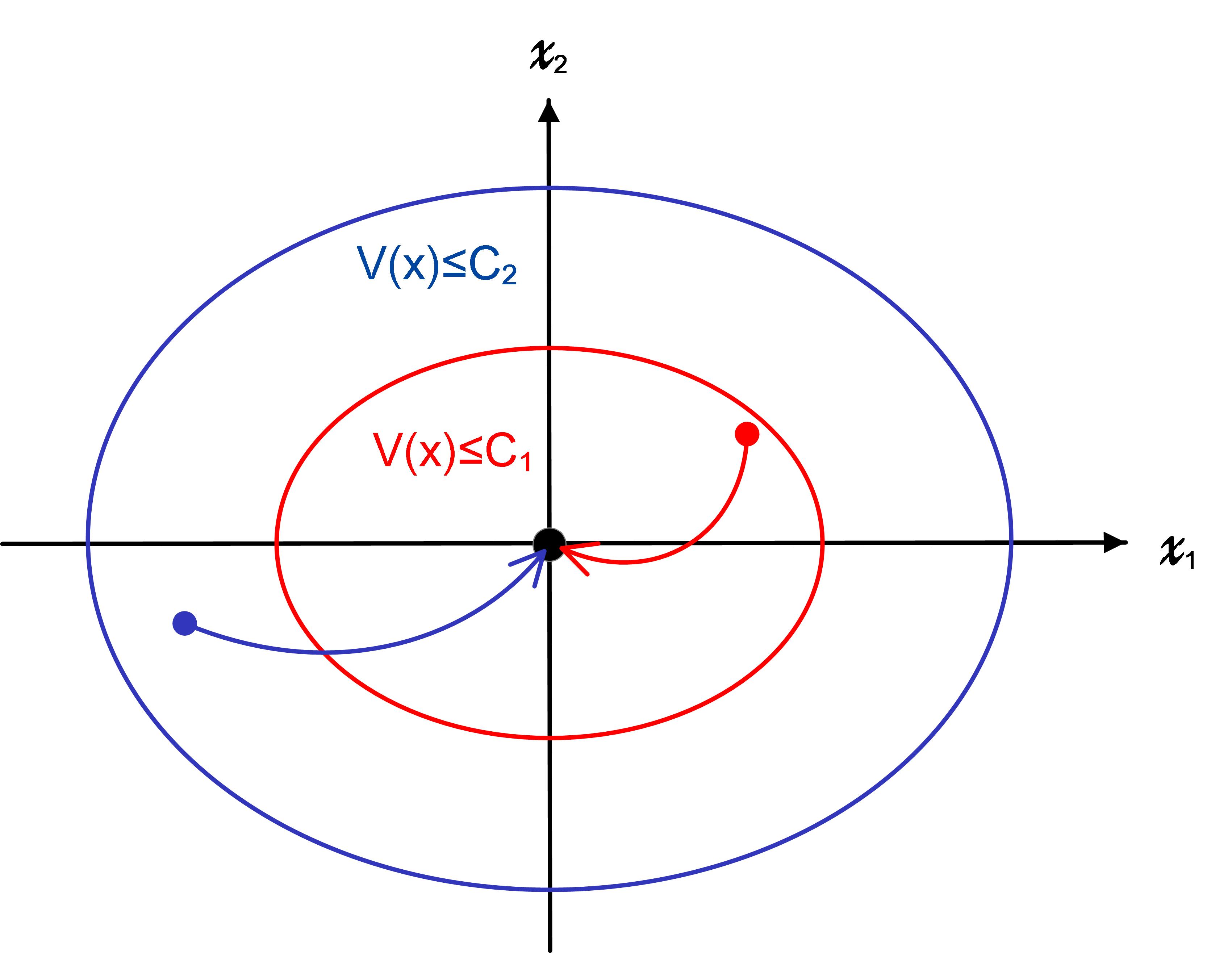
The ROA of a general dynamical system normally refers to a region where each state can converge to the stable equilibrium point as time goes to infinity. Likewise, the ROA of a power system is viewed as a set of operating states such as rotor angles and frequencies able to converge to the stable equilibrium, which corresponds to the solution of power flow problem [9, 10, 4, 11, 12, 16], after being subject to a disturbance. The corresponding convergent trajectory is regarded as a stable state trajectory. The estimation of ROA is basically dependent on the construction of Lyapunov function and its level set (see Fig. 1). In practice, constructing an analytic Lyapunov function for a nonlinear system is a challenging task.
The converse Lyapunov theorem [17] allows for estimating the value of Lyapunov function without using its analytic form. For a power system that has a stable state trajectory , , a commonly used converse Lyapunov function is [27]. We generalize converse Lyapunov function by introducing a more general function (see the definition in Appendix VI-A) and a solution trajectory in Lemma 1. The existence of such generalized Lyapunov function is guaranteed in theory (i.e., Theorem in [17]) as follows.
Lemma 1.
Without loss of generality, let be an asymptotically stable equilibrium point for the nonlinear system , where is locally Lipschitz, and is the region of attraction, then there is a continuous positive definite function such that
and
| (1) |
with
| (2) |
is a class function (see Appendix VI-A), and the level set is a compact subset of .
In Lemma 1, the dynamics of a power system normally represent that of generators which are known as swing equations [28]. Here we explicitly assume that the system dynamics are available, although our framework can be generally extended to incorporate uncertainties with a predefined complexity level, i.e., the smoothness of the unknown components, in the system’s dynamical model. Property (1) implies that the function decays over time. Equation (2) defines a stable trajectory with the initial state . More importantly, the Lyapunov function in Lemma 1 has a nice property that, by increasing the level set of , we can approach the real region of attraction (see Remark 7 for a formal explanation). Note that this property may not hold for any analytical Lyapunov function. Thus, we can leverage the converse Lyapunov function approach to obtain a better ROA by collecting more sampling points in order to enlarge the level sets.
Due to the discrete nature of sampling data, the converse Lyapunov function in Lemma 1 can be discretized and approximated as follows
| (3) |
where denotes the sampling time interval and , . The error caused by the above discretization can be further estimated (see Lemma 2 in Appendix VI-B).
While the approximated can be calculated directly based on samples, the explicit Lyapunov function is unknown. This work therefore learns this unknown Lyapunov function from the discretized counterpart. By treating and as a GP and its measurement, respectively, the estimation error can be regarded as the measurement noise. This enables us to learn the unknown Lyapunov function using the GP approach.
III GP for Learning Unknown Dynamics
The above section introduces the discretized, approximated Lyapunov function and the respective unknown Lyapunov function. In this section, we propose the GP approach for learning the unknown Lyapunov function (i.e., GP regression). Normally, a general GP regression requires a prior distribution of unknown functions specified by a mean function, a covariance function, and the probability of the observations and sampling data to obtain the posterior distribution. Without loss of generality, we consider an unknown function as a GP, which can be sequentially measured by
where refers to the observed function value for the input at the -th sampling step, and the measurement noise is zero-mean, independent and bounded by . With the GP approach, we can obtain the posterior distribution over by using sampling data in the training set .
In this work, it is assumed that the unknown Lyapunov function is a GP prior or its “complexity” can be measured by the RKHS norm. The sampling data are obtained by implementing the GP-UCB based sampling algorithm. Note that, for an existing Lyapunov function, the GP approach allows to extend the certified ROA with a given confidence level.
III-A Gaussian process and RKHS norm
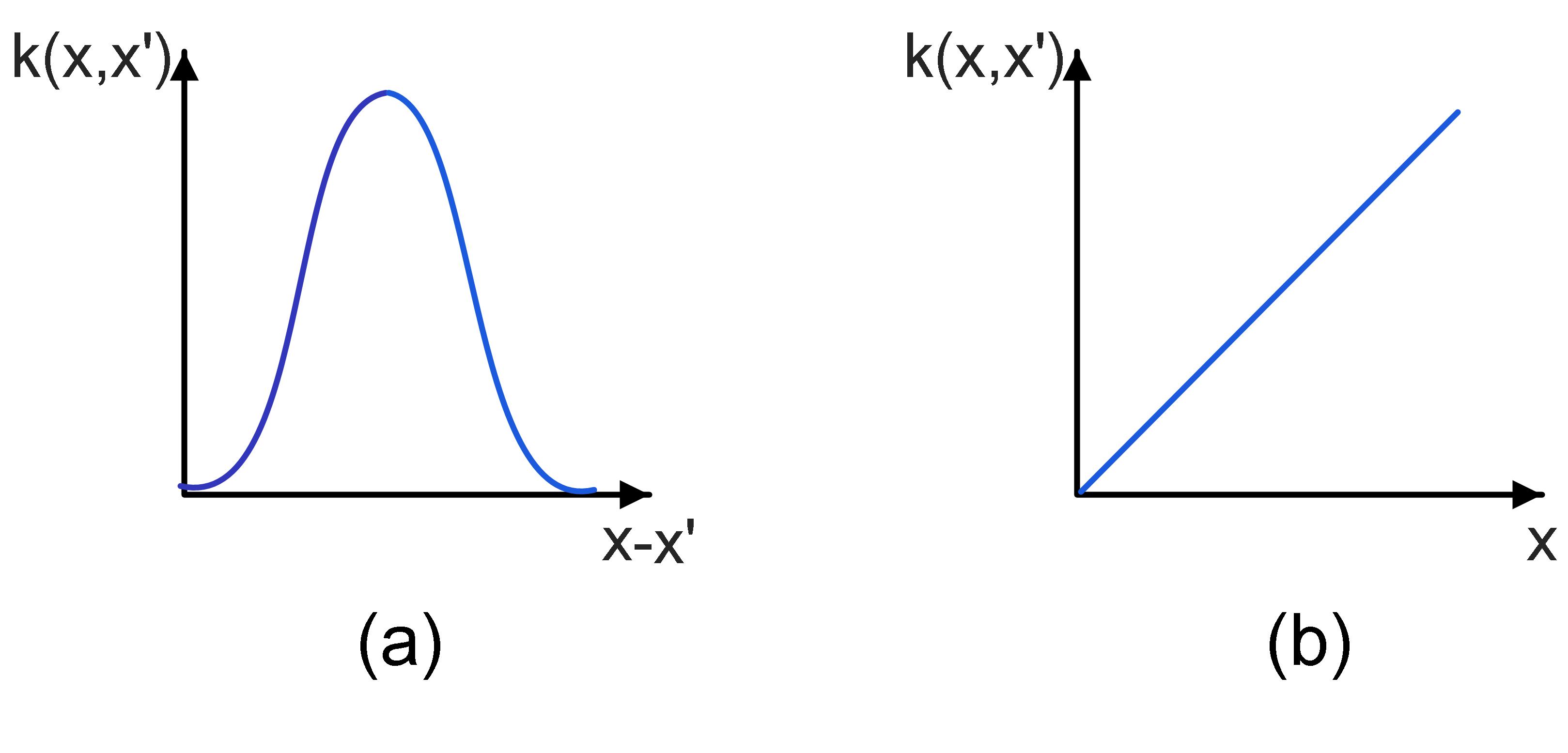
By regarding the values of as random variables, any finite collection of them is multivariate distributed in an overall consistent way. The unknown Lyapunov function can be approximated by a GP. Note that the covariance or kernel function encodes the smoothness property of from the GP (see Fig. 2). For a sample from a known GP distribution at points , with , there are the analytic formulas for mean , covariance and variance of the posterior distribution as follows [23]
| (4) |
where and is the positive definite kernel matrix .
If the prior distribution over is unknown, can be approximated by the linear combination of kernel functions in the RKHS, i.e. . The RKHS with the kernel is a complete subspace of , and its inner product is endowed with the reproducing property: , . Moreover, there exists a uniquely associated RKHS for each kernel [21]. The induced RKHS norm is used to quantify the smoothness of the function with respect to the kernel . In brief, the function gets smoother as decreases. In this work, we consider that Lyapunov functions have relatively low “complexity” or high smoothness, which can be measured by the RKHS norm.
Remark 1.
There is an interesting connection between the kernel function in RKHS and the covariance function of a GP. If the kernel function in RKHS is the same as the covariance function of a GP, the posterior mean of a GP is equivalent to the estimator of kernel ridge regression in RKHS [29]. In addition, the posterior variance of a GP can be regarded as a worst case error in RKHS.
Within the GP approach, how one samples plays an important role because the sampling rule affects the confidence level of the estimated ROA, which is the probability at least with which a trajectory initiated from an inner state of such estimated ROA will converge to the corresponding stable equilibrium. In other words, that is the probability that an estimated ROA is valid. For this work, we use the GP-UCB based sampling rule. Compared with other heuristics in GP optimization [30, 31, 32], the GP-UCB based sampling rule is able to deal with the trade-off between exploitation for optimizing the objective function and exploration for reducing the uncertainty with the guaranteed theoretical performance.
III-B GP-UCB based algorithm
For a given value of and the sampling domain , which is a subset of the state space, our goal is to maximize the region of attraction, wherein each point converges to the origin with probability at least the confident level of . Thus, a GP-UCB based algorithm is developed in Table I to select the sampling points for enlarging the ROA with a guaranteed confidence level. Specifically, a sampling point is selected in by searching for the maxima of , where the term contributes to enlarge the level set of Lyapunov function and the term allows to reduce the uncertainty of sampling region.
Essentially, the sampling rule aims to reconcile the trade-off between the exploitation for enlarging the ROA and the exploration for reducing the uncertainty of sampling region. Let the sampling point serve as the initial condition of nonlinear system , and this allows to generate a state trajectory , . If this state trajectory can converge to the origin, the point is called as a stable sampling point. Then the value of Lyapunov function at is estimated by with (3). By choosing as the training set, and for the unknown Lyapunov function can be updated according to (4). On the other hand, if the state trajectory , fails to converge to the origin, the sampling point is removed from the sampling region . The above process does not terminate until it achieves the specified number of stable sampling points.
| Input: , , , , , , , |
| Output: , , , , , |
| 1: while |
| 2: Choose |
| 3: Generate a state trajectory , |
| 4: if () |
| 5: Sample with (3) |
| 6: Update and with (4) |
| 7: Update |
| 8: else |
| 9: Update . |
| 10: end if |
| 11: end while |
Figure 3 illustrates three different sampling schemes, i.e., Scheme A, Scheme B, Scheme C which correspond to sampling points A, B, C, respectively. Mathematically, Scheme can be described as and Scheme is expressed as . In practice, Scheme is too greedy and tends to get local optima, while Scheme provides a good rule for exploring globally [23]. As a result, Scheme is designed to integrate with by adopting , where the reward function is given by
In addition, the parameter depends on the “complexity” of Lyapunov function, the sample size and information gain (see Appendix VI-C).
Remark 2.
To obtain the global maximum of in the sampling region is generally infeasible due to the non-convexity of . In practice, there are multiple ways to heuristically search for its local maxima. For instance, the local maxima can be readily identified from the finite historic dataset of sampling points instead of the region . In addition, it is expected to approach the local maxima along the gradient ascent of , and the gradient can be approximated with the finite difference method [33].
Remark 3.
For a certified ROA, it is sufficient to judge a stable sampling point if the corresponding state trajectory can overpass the boundary of this ROA without checking its convergence to the stable equilibrium point. This will reduce the computation time for selecting the stable sampling points.
IV Main Results
This section presents main theoretical results on the construction and evaluation of ROA with a given confidence level by using the GP-UCB based algorithm.
Theorem 1.
Let , and the measurement noise is bounded by . Then it holds with probability at least that
where .
Proof.
The results follow directly from Theorem 6 in [23]. ∎
Remark 4.
The RKHS norm characterizes the “complexity” or “smoothness” of the function in RKHS. If the bound of is unknown a prior, it can be computed using kernel ridge regression as , where and denotes a diagonal matrix with the diagonal elements , . Moreover, is a positive tunable parameter for controlling the smoothness of to avoid overfitting. A larger value of leads to the smoother function (see Appendix VI-D).
For a stable equilibrium point, the Lyapunov function is viewed as a GP, and Theorem 1 allows to estimate the ROA of nonlinear system with a given confidence level. If the ROA is already established according to an existing Lyapunov function , the proposed approach is applied to evaluate the stability of the region outside the ROA by treating the mismatch between and as a GP. Thus, theoretical results are summarized as follows.
Theorem 2.
Let and be an existing Lyapunov function for nonlinear system . With GP-UCB based Algorithm in Table I, it holds that
where is given by
with and
For a stable equilibrium point, the above conclusion also holds with .
Proof.
See Appendix VI-E. ∎
Remark 5.
There are alternative schemes to characterize the mismatch between the converse Lyapunov function and the existing Lyapunov function other than the difference scheme . For example, it is also feasible to adopt the proportion scheme as an unknown function for the GP learning. Essentially, a stable equilibrium point can be thought of as a special case of the ROA when the ROA shrinks into a point and thus the existing Lyapunov function becomes .
V Numerical Simulations
This section presents simulation results using the GP-UCB based algorithm for both single machine infinite bus (SMIB) system and IEEE 39 bus system. First of all, swing dynamics of a power system are introduced as follows.
V-A Power system model
Consider a -bus power system described by a set of swing equations as follows [26, 35]
| (5) |
where , and . Note that denotes the angle of the generator at bus , and the superscript represents the steady state condition or the power flow solution. The swing equation (5) describes the evolution of the phase angle due to the power mismatch between the mechanical power and the electrical power. In addition, is the neighbourhood set of bus , and denotes the susceptance of branch . The parameters and refer to inertia and damping coefficients for the machine, respectively. For a load bus , we normally assume that . In the steady state condition, the mechanical power can be expressed as . This allows us to obtain the following perturbed dynamic model
A number of approaches to assess the stability of these systems are presented in [2, 3, 5, 6, 15, 14, 13]. Here, we use an energy-like function for the above system of nonlinear differential equations as follows
and the origin (i.e., ) is locally asymptotically stable, and the certified ROA can be estimated by [26]
| (6) |
where and . In addition, denotes the Laplacian matrix of power network with weights , and is a diagonal matrix that satisfies with . Moreover, is given by with . For simplicity, the class function in Definition 1 is chosen as in order to estimate the value of converse Lyapunov function.
V-B Single machine infinite bus system
In this SMIB system, bus is the generator bus which is connected to the infinity bus where . The swing equation for this SMIB system is given by
where , , and , and thus we have and . All values are in p.u. Then the ROA can be estimated by according to (6) and it is described by the red dashed ellipse in Fig. 4. The GP-UCB based Algorithm in Table I is adopted to assess the confidence level of operating states around the certified ROA. The parameter setting is given as follows: , , , and . In addition, the squared exponential kernel or covariance function is employed to learn the unknown Lyapunov function with the unit characteristic length-scale and . Figure 5 presents the simulation result for the SMIB system. The sampling points are denoted by small green dots, and the region of operating states with confidence level at least has been marked in yellow. This implies that each state point in the yellow region converges to the origin with the probability that is not less than . It is observed that the red dashed ellipse is closely surrounded by the yellow region. Notably, the yellow region covers most sampling points outside the certified ROA except for four sampling points that are far away from the origin.

V-C IEEE 39 bus system
In order to validate the scalability of the proposed approach, numerical simulations are also conducted on the IEEE 39-bus 10-machine system (see Fig. 6), and the parameters are the same as those in [36]. Bus with a generator is assigned as the swing bus. We then consider the dynamics for the remaining machines. The detailed parameter setting and the algorithm can be found in our MATLAB code made available in GitHub [37]. Figure 7 shows the assessment result for the ROA of IEEE bus system with machines. To facilitate the visualization, we project the stable sampling points, the certified ROA and the confidence region onto distinct two-dimensional planes, respectively. Essentially, each plane acts as a cross section to showcase the profile of confidence region and certified ROA with respect to a different machine. In each panel of Fig. 7, the state points inside the red dashed ellipse is guaranteed to converge to the origin, while those in the yellow region are asymptotically convergent with the probability at least .
By Monte Carlo like estimate, the volume of yellow region is about times larger than that of the certified ROA. This achievement is due to the large number of state dimensions or the size of the considered dynamical system. Note that this comparison is not entirely fair as the certified ROA can ensure that the system state will always converge to the stable equilibrium if it starts from the inside, while our estimated yellow region is only confident.
Similar to the case of the SMIB system, the yellow region does not cover the state points that are relatively far away from the origin. Actually, the profile of yellow regions largely depends on the distribution and size of sampling points as well as the choice of kernel functions for GP learning.


V-D Discussions on computational cost
The computational burden associated with GP-UCB algorithm is mostly due to two processes: solving the dynamical equation or swing equation using ODE solvers, and GP optimization presented in (4). While the former depends heavily on the system size, the dimension of differential equation for power systems does not result in the visible increase of computational cost in GP optimization. Indeed, the computational cost is essentially immune to the dimension of power system dynamics. This is because the computation burden largely results from the operation of matrix inverse in (4), where the size of kernel matrix mainly depends on the number of sampling points rather than the dimension of power system dynamics. With Matlab 2017b in the desktop (Intel i7-3770 CPU 3.40GHz and installed RAM 8GB), it takes around minutes for IEEE -bus system and seconds for the SMIB system in our simulations. For the large-size sampling data, many efficient approaches for training the GP with the desirable performance [38] are available. For instance, the sparse representation of GP model is developed to overcome the limitations for large data sets via the sequential construction of a sub-sample of the entire sampling data [39].
VI Conclusions and Future Work
In this paper, we investigated the problem of estimating the ROA for power systems. By treating the unknown Lyapunov function as a Gaussian Process, we assessed state stability of power systems with the aid of the converse Lyapunov function. For an existing Lyapunov function, our approach allows for extending the pre-existing ROA with a provable confidence level. In addition, a GP-UCB based algorithm was developed to deal with the trade-off between exploration and exploitation in selecting stable sampling points. Numerical simulations are conducted to validate the proposed approach on the IEEE test cases.
In the next step, we will consider the online learning applications of unknown dynamics in practical power systems and the real-time prediction and stability assessment. This requires the creation of an efficient numerical algorithm with the aid of Gaussian Process and the converse Lyapunov function, which introduces the second part of this work. Another improvement is to optimally rescale state variables to be aligned to the shape of the real ROA which is not equal in all dimensions.
Acknowledgement
The work of Chao Zhai and Hung Nguyen is supported by NTU SUG.
Appendix
This section provides a mathematical definition of the class function and theoretical proofs for Lemma 2, Lemma 3 and Theorem 2, respectively. First of all, the definition is presented as follows.
VI-A The class function
Definition 1.
The class function consists of all continuous functions which satisfy the following conditions:
- 1.
, .
- 2.
, and .
- 3.
, , such that .
Remark 6.
Condition in Definition 1 indicates that the first two derivatives of the class function exist and are continuous. Condition implies that is a strictly increasing function. In addition, Condition aims to impose the restriction on the rate of .
Remark 7.
The construction of in Lemma 1 allows us to obtain an important property on the region of attraction (i.e., ). Specifically, , we have , which implies and . Thus, we have and . In addition, it is guaranteed that , . This indicates and thus . It follows that . Considering that the constant can be sufficiently large, we have .
VI-B An upper bound of discretizing error
An upper bound of the estimation error due to discretizing converse Lyapunov function is given below.
Lemma 2.
Let be Hurwitz. There are positive constants , , and such that the following inequality holds
| (7) |
The proof is given below.
that
By the trapezoidal rule for numerical integration in the interval [40], the error bound is given by
where , . Considering that is Hurwitz, is an exponentially stable equilibrium point from Corollary in [17]. This implies that there are positive constants and , such that , . In terms of Condition of the class function in Definition 1, there is the positive constant such that
Therefore, we obtain
This completes the proof.
We discuss some notes on the Inequality (7) in the following remark.
Remark 8.
Remark 9.
The first partial derivative of with respect to time is given by
where . And the second partial derivative of with respect to time is given by
| (8) |
where and
Equation (8) enables us to estimate the upper bound of in and obtain the constant .
VI-C Information gain
To quantify the reduction in uncertainty on from observations , the information gain is introduced for a Gaussian process as follows
where is the covariance matrix of with the sample set . Let denote the upper bound of for the sample set with . That is
Actually, is related to the choice of kernel functions .
Lemma 3.
For , it holds that
when .
Proof.
Since is a positive definite kernel matrix, it follows that
where , are all positive eigenvalues of . Considering that , , we have
Because of and , we obtain
Therefore, we get
and
This completes the proof. ∎
VI-D Computation of the RKHS norm
Kernel ridge regression can be formulated as a regularized empirical risk minimization problem over the RKHS as follows
It follows from Theorem in [21] that there is a unique solution to the above minimization problem, and the solution is given by with the coefficient vector . Thus, can be computed by
By substituting the vector and the positive semidefinite matrix , we have
VI-E Proof of Theorem 2
The proof consists of two parts. The first part aims to estimate the ROA for a stable equilibrium point, and the second part centers on the ROA for the case of an existing Lyapunov function .
Since is an asymptotically stable equilibrium point for the nonlinear system , Lemma 1 guarantees the existence of Lyapunov function . Considering a sequence of sampling points , ,…, in that can generate the stable state trajectory, the values of , can be estimated as according to Equation (3). By treating as the observations of a GP, the measurement noise is uniformly bounded by , which satisfies
from Lemma 2. In addition, it follows from Theorem 1 that with probability at least , the inequality
holds, where and from Lemma 3. This allows us to deduce that the inequality
holds with probability at least . Then we define a level set for the converse Lyapunov function as , which includes all the stable state trajectories of sampling points , and is a compact subset of the region of attraction (i.e., ). Thus, if we have , the inequality holds with probability at least , which implies , with
Considering that , we obtain , .
Considering that is an existing Lyapunov function for the nonlinear system with the certified ROA , it is suggested that the origin is an asymptotically stable equilibrium point. This ensures the existence of a converse Lyapunov function according to Lemma 1. Define as an unknown function for the GP learning. By observing the measurements as a GP at the sampling points , according to GP-ROA based algorithm in Table I, it follows from Theorem 1 that the inequality
holds with probability at least . By replacing with , we obtain
In light of the proof for a stable equilibrium point, it is concluded that for any , the inequality holds. This completes the proof.
References
- [1] Nguyen, Hung D and Vu, Thanh Long and Slotine, Jean-Jacques and Turitsyn, Konstantin, 2017. Contraction analysis of nonlinear dae systems. arXiv preprint arXiv:1702.07421
- [2] Parikshit Pareek, Konstantin Turitsyn, Krishnamurthy Dvijotham, Hung D Nguyen, 2018. A Sufficient Condition for Small-Signal Stability and Construction of Robust Stability Region. arXiv preprint arXiv:1811.03805
- [3] Dongchan Lee, Hung D Nguyen, Krishnamurthy Dvijotham, Konstantin Turitsyn, 2018. Convex Restriction of Power Flow Feasibility Sets. arXiv preprint arXiv: 1803.00818
- [4] Dhagash Mehta, Hung D. Nguyen, Konstantin Turitsyn, 2016. Numerical Polynomial Homotopy Continuation Method to Locate All The Power Flow Solutions. IET Generation, Transmission & Distribution, 10.12 (2016): 2972-2980.
- [5] Hung D Nguyen, Konstantin Turitsyn, 2015. Robust stability assessment in the presence of load dynamics uncertainty. IEEE Transactions on Power Systems, 31.2 (2015): 1579-1594.
- [6] Hung D Nguyen, Konstantin Turitsyn, 2015, Voltage multistability and pulse emergency control for distribution system with power flow reversal. IEEE Transactions on Smart Grid 6.6 (2015): 2985-2996.
- [7] Bogodorova, Tetiana and Vanfretti, Luigi and Turitsyn, Konstantin, 2015. Bayesian parameter estimation of power system primary frequency controls under modeling uncertainties. IFAC-PapersOnLine, 48(28), pp. 461–465.
- [8] T. L. Vu and K. Turitsyn, 2016. Lyapunov Functions Family Approach to Transient Stability Assessment. IEEE Transactions on Power Systems, 31(2), pp. 1269-1277.
- [9] Zheng Zhang, Hung Dinh Nguyen, Konstantin Turitsyn, Luca Daniel, 2015. Probabilistic power flow computation via low-rank and sparse tensor recovery. arXiv preprint arXiv:1508.02489
- [10] Lesieutre, Bernard and Wu, Dan, 2015. An efficient method to locate all the load flow solutions-revisited. 53rd Annual Allerton Conference on Communication, Control, and Computing (Allerton), pp. 381–388.
- [11] J. Liu and B. Cui and D.K. Molzahn and C. Chen and X. Lu, 2019. Optimal Power Flow for DC Networks with Robust Feasibility and Stability Guarantees.
- [12] Aolaritei, Liviu and Bolognani, Saverio and Dörfler, Florian, 2017. A distributed voltage stability margin for power distribution networks. IFAC-PapersOnLine, 50(1), pp. 13240–13245.
- [13] P. Vorobev and P. Huang and M. Al Hosani and J. L. Kirtley and K. Turitsyn, 2018. High-Fidelity Model Order Reduction for Microgrids Stability Assessment. IEEE Transactions on Power Systems, 33(1), pp. 874-887.
- [14] Tuyen, Nguyen Duc and Fujita, Goro and Funabashi, Toshihisa and Nomura, Masakatsu, 2017. Analysis of transient-to-island mode of power electronic interface with conventional dq-current controller and proposed droop-based controller. Electrical Engineering, 99(1), pp. 47–57.
- [15] Tran, Thanh Son and Nguyen, Duc Tuyen and Fujita, Goro, 2019. The Analysis of Technical Trend in Islanding Operation, Harmonic Distortion, Stabilizing Frequency, and Voltage of Islanded Entities. Resources, 8(1).
- [16] Ali, Mazhar and Dymarsky, Anatoly and Turitsyn, Konstantin, 2017. Transversality Enforced Newton Raphson Algorithm for Fast Calculation of Maximum Loadability. IET Generation, Transmission & Distribution.
- [17] Khalil, H.K. and Grizzle, J.W., 2002. Nonlinear Systems (Vol. 3). Upper Saddle River, NJ: Prentice Hall.
- [18] Izumi, S., Somekawa, H., Xin, X. and Yamasaki, T., 2018. Estimation of regions of attraction of power systems by using sum of squares programming. Electrical Engineering, 100(4), pp. 2205-2216.
- [19] Chesi, G., 2011. Domain of attraction: analysis and control via SOS programming (Vol. 415). Springer Science & Business Media.
- [20] Bobiti, R. and Lazar, M., 2018. Automated-Sampling-Based Stability Verification and DOA Estimation for Nonlinear Systems. IEEE Transactions on Automatic Control, 63(11), pp. 3659-3674.
- [21] Kanagawa, M., Hennig, P., Sejdinovic, D. and Sriperumbudur, B.K., 2018. Gaussian processes and kernel methods: A review on connections and equivalences. arXiv preprint arXiv:1807.02582.
- [22] Rasmussen, C.E. and Nickisch, H., 2010. Gaussian processes for machine learning (GPML) toolbox. Journal of Machine Learning Research, 11(Nov), pp. 3011-3015.
- [23] Srinivas, N., Krause, A., Kakade, S.M. and Seeger, M.W., 2012. Information-theoretic regret bounds for gaussian process optimization in the bandit setting. IEEE Transactions on Information Theory, 58(5), pp. 3250-3265.
- [24] Berkenkamp, F., Krause, A. and Schoellig, A.P., 2016. Bayesian optimization with safety constraints: safe and automatic parameter tuning in robotics. arXiv preprint arXiv:1602.04450.
- [25] Gibbs, M.N. and MacKay, D.J., 2000. Variational Gaussian process classifiers. IEEE Transactions on Neural Networks, 11(6), pp. 1458-1464.
- [26] Münz, U. and Romeres, D., 2013. Region of attraction of power systems. IFAC Proceedings Volumes, 46(27), pp. 49-54.
- [27] Jones, M., Mohammadi, H. and Peet, M. M., 2017, December. Estimating the region of attraction using polynomial optimization: A converse Lyapunov result. In 2017 IEEE 56th Annual Conference on Decision and Control (CDC) (pp. 1796-1802). IEEE.
- [28] Kundur, P., Balu, N. J. and Lauby, M. G., 1994. Power System Stability and Control (Vol. 7). New York: McGraw-Hill.
- [29] G. S. Kimeldorf and G. Wahba. A correspondence between Bayesian estimation on stochastic processes and smoothing by splines. The Annals of Mathematical Statistics, 41(2): 495-502, 1970.
- [30] Mockus, J., 1975. On Bayesian methods for seeking the extremum. In Optimization Techniques IFIP Technical Conference (pp. 400-404). Springer, Berlin, Heidelberg.
- [31] Mockus, J., 2012. Bayesian Approach to Global Optimization: Theory and Applications (Vol. 37). Springer Science & Business Media.
- [32] Brochu, E., Cora, V. M. and De Freitas, N., 2010. A tutorial on Bayesian optimization of expensive cost functions, with application to active user modeling and hierarchical reinforcement learning. arXiv preprint arXiv: 1012.2599.
- [33] Stoer, J. and Bulirsch, R., 2013. Introduction to Numerical Analysis (Vol. 12). Springer Science & Business Media.
- [34] R. D. Zimmerman, C. E. Murillo-Sánchez, and R. J. Thomas, “MATPOWER: Steady-State Operations, Planning and Analysis Tools for Power Systems Research and Education,” IEEE Transactions on Power Systems, vol. 26, no. 1, pp. 12-19, Feb. 2011.
- [35] Sauer, P.W. and Pai, M.A., 1998. Power System Dynamics and Stability (Vol. 101). Upper Saddle River, NJ: Prentice hall.
- [36] Dörfler, F., Jovanović, M.R., Chertkov, M. and Bullo, F., 2014. Sparsity-promoting optimal wide-area control of power networks. IEEE Transactions on Power Systems, 29(5), pp. 2281-2291.
- [37] https://github.com/Chaocas/ROA-for-Power-Systems
- [38] Liu, H., Ong, Y.S., Shen, X. and Cai, J., 2018. When Gaussian process meets big data: A review of scalable GPs. arXiv preprint arXiv:1807.01065.
- [39] Csato, L. and Opper, M., 2002. Sparse on-line Gaussian processes. Neural computation, 14(3), pp. 641-668.
- [40] Atkinson, K. E., 2008. An introduction to Numerical Analysis. John Wiley & Sons.