A Probabilistic Approach to Kepler Completeness and Reliability for Exoplanet Occurrence RatesJournal: AAS JournalsFacilities: KeplerJupyter, emcee (Foreman-Mackey et al. 2013), KeplerPorts (Burke & Catanzarite 2017)
Abstract
Exoplanet catalogs produced by surveys suffer from a lack of completeness (not every planet is detected) and less than perfect reliability (not every planet in the catalog is a true planet), particularly near the survey’s detection limit. Exoplanet occurrence rate studies based on such a catalog must be corrected for completeness and reliability. The final Kepler data release, DR25, features a uniformly vetted planet candidate catalog and data products that facilitate corrections. We present a new probabilistic approach to the characterization of Kepler completeness and reliability, making full use of the Kepler DR25 products. We illustrate the impact of completeness and reliability corrections with a Poisson-likelihood occurrence rate method, using a recent stellar properties catalog that incorporates Gaia stellar radii and essentially uniform treatment of the stellar population. Correcting for reliability has a significant impact: the exoplanet occurrence rate for orbital period and radius within 20% of Earth’s around GK dwarf stars, corrected for reliability, is , whereas not correcting results in — correcting for reliability reduces this occurrence rate by more than a factor of two. We further show that using Gaia-based vs. DR25 stellar properties impacts the same occurrence rate by a factor of two. We critically examine the the DR25 catalog and the assumptions behind our occurrence rate method. We propose several ways in which confidence in both the Kepler catalog and occurrence rate calculations can be improved. This work provides an example of how the community can use the DR25 completeness and reliability products.
Keywords:
Kepler — DR25 — exoplanets — exoplanet occurrence rates — catalogs — surveysI Introduction
The Kepler space telescope (Borucki et al. 2010; Koch et al. 2010) has delivered unique data that enables the characterization of exoplanet population statistics, from hot Jupiters in short-period orbits to terrestrial-size rocky planets in orbits with periods up to one year11 1 https://exoplanetarchive.ipac.caltech.edu/docs/occurrence_rate_papers.html. By observing 150,000 stars nearly continuously for four years looking for transiting exoplanets, Kepler detected several thousand planet candidates (PCs) (Thompson et al. 2018), leading to the confirmation or statistical validation of over 2,300 exoplanets. This rich trove of exoplanet data has delivered many insights into exoplanet structure and formation, and promises deeper insights with further analysis. One of the most exciting insights to be gained from Kepler data is the occurrence rate of temperate, terrestrial-size planets orbiting Sun-like stars (often referred to as ). This occurrence rate is also a critical input to the design of future space telescopes designed to discover and characterize habitable exoplanets, such as HabEx and LUVOIR.
Fully exploiting Kepler data requires a thorough understanding of how well it reflects the underlying exoplanet population. There are several ways in which the Kepler planet candidate catalog does not directly measure the real planet population:
- •
the catalog is incomplete, missing real planets
- •
it may be unreliable, with the planet candidate catalog being polluted with false positives
- •
it may be inaccurate due to observational errors leading to incorrect planet properties.
Lack of completeness and reliability are particularly acute at the Kepler detection limit, which happens to coincide with the period and radius of Earth-Sun analog exoplanets. We therefore focus our attention on a period and radius range spanning the Kepler detection limit.
In this paper we address vetting incompleteness, a significant component of incompleteness caused by incorrectly classifying detected true planets as false positives, and vetting reliability, caused by incorrectly classifying detections as planets candidate when they are in fact not true planets. We address accuracy by using new, uniformly determined stellar properties based in part on Gaia observations, described in §III.1.
We focus our analysis on the final Kepler data release DR25 (Thompson et al. 2018) and its associated planet candidate catalog22 2 https://exoplanetarchive.ipac.caltech.edu. DR25 contains several products designed to support the characterization of the completeness and reliability of the DR25 planet candidate catalog. The primary contribution of this paper is a new probabilistic approach to using the DR25 completeness and reliability products to characterize vetting completeness and reliability. We illustrate the impact of completeness and reliability with standard occurrence rate computations, and examine the impact on occurrence rates due to changes in various assumptions. This is the first occurrence rate computation that fully uses the DR25 completeness and reliability products to characterize vetting reliability.
I.1 Previous Work
Kepler’s survey of the Cygnus field involved four years of data collection and another four years of pipeline development, data processing, and survey characterization, culminating in the final deliveries referred to as Data Release 25 (DR25). Incremental data deliveries enabled preliminary science investigations, and several occurrence rate studies were executed as the survey progressed. The simplest, first-look estimates used Gaussian cumulative distribution functions (CDF) as proxies for pipeline completeness (Borucki et al. 2011), restricted samples where completeness was assumed to be near unity (Howard et al. 2012), and linear approximations to a Gaussian CDF (Fressin et al. 2013). Lacking a full characterization of the Kepler pipeline, others employed independent detection pipelines, including injection and recovery experiments operating on flux light curves to quantify the detection completeness (Petigura et al. 2013; Foreman-Mackey et al. 2014; Dressing & Charbonneau 2015). Hsu et al. 2018 performed an occurrence rate calculation using approximate Bayesian computation (ABC) and Zink & Hansen 2019 computed a habitable zone occurrence rate taking into account the effect of planet multiplicity on completeness.
The performance of the Kepler pipeline was characterized incrementally as more data were collected using transit injection and recovery operating on raw pixel fluxes as described in Section II.1 (Christiansen et al. 2013; Christiansen et al. 2015; Christiansen et al. 2016; Christiansen 2017). These early studies provided positive feedback to the Kepler pipeline whereby deficiencies were identified and improved upon (Twicken et al. 2016). Occurrence rate calculations using 16 out of 17 quarters of data and the associated pipeline completeness offered a benchmark computation for testing methodologies and comparing independent pipelines (Burke et al. 2015). Systematic errors were explored and the tallest tent poles were identified. Among these tall tent poles were two standouts: stellar property uncertainties and catalog reliability.
The first studies to include a treatment of catalog reliability focused on identifying astrophysical false positives either deterministically through follow-up observations (Santerne et al. 2012) or probabilistically via population synthesis (Morton & Johnson 2011; Morton & Swift 2014; Morton et al. 2016). And while most treatments culled or weighted the planet population, others sought to model both the planet and astrophysical sources as part of the planet occurrence estimation (Fressin et al. 2013), with Farr et al. 2014 applying a mixture model approach. These efforts used idealized models of the false positive and false alarm populations. An extremely useful astrophysical false positive probability statistic was developed by Morton et al. 2016.
The most significant effort to characterize the reliability of the Kepler planet candidate catalog to date is the final Kepler DR25 catalog paper Thompson et al. 2018. The DR25 catalog includes a Robovetter score which estimates the confidence with which the Robovetter vetted a TCE. Thompson et al. 2018 suggests that restricting occurrence rate studies to high-Robovetter-score planet candidates avoids the problem of low-reliability candidates (we test this approach in §VI.4.2). Hsu et al. 2018 and Mulders et al. 2018 apply this high-score approach in their occurrence rate studies.
Burke et al. 2019 analyzes DR25 reliability using the inverted and scrambled data, approaching reliability characterization via kernel density estimation. The focus of Burke et al. 2019 is how reliability impacts statistical exoplanet validation.
I.2 This Paper
The primary purpose of this paper is to present a probabilistic characterization of Kepler vetting completeness (§IV.2) and reliability against false alarms (§V.1) and show the impact on standard occurrence rate computations. This probabilistic analysis is robust against sparse data and resolves detailed structure of the dependence of vetting completeness and reliability on orbital period and transit signal strength. We explore the impact of using this characterization to correct occurrence rates based on Kepler data by performing a standard Poisson-likelihood-based occurrence rate, following Burke et al. 2015. Our characterization depends on the exoplanet population, which in turn depends on the parent stellar sample that is searched for planets. We restrict our analysis to GK dwarf stars.
Our method of accounting for completeness and reliability proceeds by executing the following steps:
- •
Select a subset of the target star population, which will be our parent population of stars that are searched for planets. We apply various cuts intended to select well-behaved and well-observed stars, and we restrict our analysis to GK dwarfs, as described in §III.1.
- •
Use the injected data to characterize vetting completeness, described in §IV.2.
- •
Compute the summed detection completeness, incorporating vetting completeness, described in §IV.1.
- •
Use observed, inverted and scrambled data to characterize false alarm reliability, described in §V.1.
- •
Assemble the collection of planet candidates, including computing the reliability of each candidate from the false alarm reliability and False Positive Probability.
- •
Compute the desired occurrence rates, presented in §VI.
We perform our completeness and reliability analysis on the planet radius range . We perform our completeness analysis on the period range days and reliability analysis on the period range days. Our occurrence rates are focused on illustrating the impact of vetting completeness and reliability where both are low, so our occurrence rates are analyzed for days and .
Following an introduction to the details of completeness, reliability and the data products that support their computation in §II, this paper has four major parts: §III assembles the stellar and planet catalogs we use in our analysis. We choose a stellar catalog that incorporates Gaia stellar radii and features an essentially uniform treatment of the parent stellar sample. §IV describes catalog completeness and describes our characterization of vetting completeness. §V describes our characterization of catalog reliability. In §VI we perform our baseline occurrence rate computations corrected for vetting completeness, emphasizing the difference between correcting and not correcting for reliability. We then explore alternative occurrence rate calculations, including using an alternative stellar properties catalog, demonstrating the impact of not correcting for vetting completeness and restricting our analysis to planet candidates with Robovetter score .
Throughout this paper we present results with confidence intervals that are the 14th and 86th percentiles of posterior distributions resulting from MCMC analysis using fixed inputs. These confidence intervals do not account for uncertainties in the inputs. We address the issue of uncertainties in the inputs in §VI.3.
All results reported in this paper were produced with Python code, mostly in the form of Python Jupyter notebooks, found at the paper GitHub site33 3 https://github.com/stevepur/DR25-occurrence-public.
II Completeness, Reliability and Occurrence Rates,
As described above, completeness has two components. Detection completeness is the fraction of true planets that are detected by the Kepler pipeline. Vetting completeness is the fraction of detected true planets that are correctly vetted as planet candidates. Vetting reliability is the fraction of vetted planet candidates that are true planets.
During catalog creation, the reliability of the planet candidate catalog is increased by detecting and removing false positives using a variety of tests. When the transit signal is weak it can be difficult for these tests to distinguish false positives from true planets, so maximizing reliability via stringent tests can cause true planets to be classified as false alarms, reducing vetting completeness. The DR25 catalog addressed this problem with uniform automated vetting via the Robovetter, using tests that were tuned to strike a balance between vetting completeness and reliability. This uniform automated vetting made it possible to vet synthetic and modified data sets designed to statistically mimic true planets and false positives, described in §II.1, in exactly the same way that the observed data was vetted. In this way the completeness and reliability of the planet candidate catalog can be measured and corrected in occurrence rates.
We distinguish two broad classes of phenomena that pollute the planet candidate catalog:
- •
Astrophysical False Positives, such as grazing or eclipsing binaries, which produce a planet-transit-like signal with a regular ephemeris in observed light curves that are not due to planetary transits. There has been extensive effort to identify and remove such false positives from Kepler catalogs (Morton & Johnson 2011; Bryson et al. 2013; Fressin et al. 2013; Coughlin et al. 2014; Morton et al. 2016; Thompson et al. 2018, e.g.,), and for high SNR transits the resulting removal of astrophysical false positives is very effective. For low SNR, however, it is more difficult to distinguish astrophysical false positives from true planetary transits. In this paper we address astrophysical false positives via the probabilistic evaluation of Morton et al. 2016.
- •
False Alarms, which trigger a transit detection with a regular ephemeris, but are not due to regularly repeating astrophysical phenomena. The dominant source of false alarms in Kepler data is instrumental artifacts. There are two important classes of instrumental artifacts that have been identified as responsible for the overwhelming majority of false alarms at long periods: rolling bands and statistical and pixel fluctuations.
- –
Rolling bands (Van Cleve & Caldwell 2009; Caldwell et al. 2010) are thermally dependent quasi-sinusoidal electrical signals in the output of the Kepler CCDs. As the Kepler telescope slowly changes its attitude relative to the Sun, different parts of the photometer are illuminated. While the thermal insulation of the telescope and electronics is very good, it is not perfect and the resulting thermal variations cause the rolling bands to slowly move across the CCDs, often introducing signals that look very much like transits. Because Kepler’s attitude is determined by its 372-day orbit, rolling bands often induce transit-like signals that repeat with a nearly regular ephemeris with an approximately 372-day period. This is the cause of the sharp peak of TCEs in the left panel of Figure 1. Rolling bands are highly focal plane position dependent: some Kepler CCD channels have much more severe rolling bands than others.
- –
Statistical and pixel fluctuations are independent, unrelated dips in light curves due to cosmic ray hits, single transits, and statistical fluctuations that trigger transit detections when they accidentally fall into a regular ephemeris. This class of false alarms becomes much more common for long-period ephemerides because they only require three or four events to fall on a regular ephemeris, and explains the broader “shoulders” of the tall peak in the left panel of Figure 1.
- –

In addition, stellar variability triggers false alarm transit detections on a regular ephemeris, typically at short periods. False positives and false alarms are treated differently in our analysis, as described in §V.
In an ideal world, measuring planet occurrence rates from Kepler data would be simple — divide the number of detected planets by the number of observed stars, correcting for the geometrical probability of a planet transit. To get an accurate occurrence rate, however, this approach must be corrected for completeness and reliability. This correction can be large for Earth-Sun analog systems, which are at the Kepler detection limit where both completeness and reliability are very low. Specifically, instrumental false alarms are a significant source of false transit detections in the long-period, low signal-to-noise (SNR) region of most interest for habitable zone occurrence rate studies for G and K dwarf stars. In this regime, as shown in Figure 1, the number of instrumental false alarms is very large compared to the expected population of true exoplanet detections.
II.1 DR25 Vetting and Reliability Products
The DR25 planet candidate catalog (Thompson et al. 2018) contains 4034 identified planet candidates (PCs) out of 8054 Kepler Objects of Interest (KOIs). The KOIs were extracted from a catalog of 34,032 transit detections called threshold crossing events (TCEs), which are periodic transit-like events (Jenkins 2002, as identified by a matched filter;) that have a combined signal strength above a threshold (typically ). Identification of the PCs from the KOIs was performed by a fully automated Robovetter. The Robovetter applies a variety of tests to each TCE, many of which are based on the synthetic test datasets described below, and planet candidates are TCEs that pass all tests while following a logic tree. Such automated vetting (and transit detection) is critical for the production of a statistically uniform catalog that is amenable to statistical correction for completeness and reliability.
The DR25 completeness products are based on injected data — a ground-truth of transiting planets is obtained by injecting transit signals with specific characteristics on all observed stars at the pixel level (Christiansen 2017). This data is then analyzed by the Kepler detection pipeline to produce a catalog of detections at the injected ephemerides called injected and recovered TCEs, which are then sent through the same Robovetter used to identify planet candidates. The fraction of injected transits that are recovered as TCEs measures detection completeness, while the fraction of recovered TCEs that are vetted as planet candidates measures vetting completeness. A large number of transits were also injected on a small number of target stars to measure the dependence of completeness on transit parameters and stellar properties. This data is used to create high-resolution, per-target-star detection contours described in §IV.1, providing completeness for each target star as a function of planet orbital period and radius (Burke & Catanzarite 2017).
The rate of false alarms, measured for the first time in DR25, are characterized by manipulating observed data so that it contains no true astrophysical transiting exoplanet signals, creating a ground-truth in which any TCE or vetted planet candidate is an instrumental false alarm. There are two basic manipulations that create the data used to characterize the rate of false alarms:
- •
Data inversion flips the light curves “upside down” so that true transiting signals increase in brightness and are therefore not identified as transits. This is believed to preserve the quasi-sinusoidal rolling bands described above. The distribution of TCEs detected in the inverted data reproduces well the sharp peak at a period of 372 days that is seen in the distribution of observed TCEs in the left panel of Figure 1.
- •
Data scrambling shuffles the Kepler observational quarters in a way that destroys the regular ephemeris of astrophysical transit signals, preventing their detection by the Kepler pipeline. While this also prevents the detection of the same false alarms that are detected in the original observed data, it is believed to preserve the statistics of detections due to statistical and pixel fluctuations. The distribution of TCEs detected in the scrambled data is very similar to the broad shoulder near periods of one year in the distribution of observed TCEs seen in the left panel of Figure 1. Three different shuffles of the Kepler data are available.
The DR25 Robovetter uses a number of metrics to identify instrumental false alarms, and the inverted and scrambled data sets were used to tune their pass/fail thresholds. For an extensive discussion, see Thompson et al. 2018.
For many Robovetter metrics, the distribution of values from the inverted/scrambled data overlaps the distribution of values in the observed data, making it difficult to distinguish false alarms from true planets, particularly at long period and low SNR. This results in low reliability in some parameter spaces of the Kepler planet candidate catalog, especially near the detection limit. An effort to characterize this catalog reliability is described in Section 4 of Thompson et al. 2018. The work presented in this paper is an attempt to improve on this characterization.
III Input Catalogs
III.1 The Stellar Catalog
Our occurrence rate starts with a parent stellar population of GK dwarf stars that is searched for planetary transits. The properties of each star determine the likelihood that a transiting planet of a given size will be observed. The radius of the planet is derived from the fitted radius ratio and stellar radius. While the most accurate stellar properties for each star is desirable for understanding the properties of the transiting planet, a statistical occurrence rate requires the most uniform stellar properties possible. This is an issue for Kepler data because target stars with actual transit detections are much better characterized than most targets stars without transit detections. This can potentially lead to unknown biases in the estimated detection completeness of §IV.2.
The stellar catalog associated with the DR25 exoplanet catalog, Q1-Q17 DR25 (with supplement)44 4 https://exoplanetarchive.ipac.caltech.edu/docs/Kepler_stellar_docs.html, is based on heterogeneous observations, with some stars having properties derived from asteroseismic data, others from spectral data, and most from photometric data, all fitted to Dartmouth isochrones (Mathur & Huber 2016; Mathur et al. 2017). Berger et al. 2018 combined the DR25 stellar catalog with Gaia parallaxes (Lindegren et al. 2018) to improve stellar radii, yielding an average radius precision of less than 10% for most Kepler stars. However, the adopted effective temperatures were still heterogeneous, and no revisions of other stellar properties such as mass and surface gravities were performed.
For our parent stellar population we use the stellar catalog of Berger et al. 2020, which extends Berger et al. 2018 by deriving a full set of stellar properties from isochrone fitting using broadband photometry, Gaia parallaxes and spectroscopic metallicities where available. This catalog is based on the homogeneous derivation of temperatures and luminosities, which previously have been the dominant sources of systematic errors in stellar (and thus planet) radii. These consistently fitted stellar properties provide more uniformly derived stellar radii over the entire parent population than the DR25 stellar properties. We recompute the 4-parameter stellar limb darkening model coefficients using these stellar properties via the table tableeq5.dat in Claret & Bloemen 2011, assuming a microturbulent velocity of 2 km s-1. In §VI.4.1 we compare the resulting baseline occurrence rates with those using the DR25 stellar properties. We address the issue of possible bias against small planets in the Berger et al. 2020 catalog in §VI.4.1 and Appendix C.
Because we require information such as observational completeness from the DR25 catalog and the binary flag from Berger et al. 2018 for each target star, we merge Berger et al. 2020, the DR25 stellar catalog (with supplement), and Berger et al. 2018, keeping only the 177,798 stars that are in all three catalogs. We remove possibly poorly characterized, binary and evolved stars using the following cuts:
- •
Remove stars with Berger et al. 2020 goodness of fit (iso_gof) and Gaia Renormalized Unit Weight Error (RUWE, provided by Berger et al. 2020) (Lindegren 2018) , leaving 162,219 stars. iso_gof measures the quality of the Berger et al. 2020 isochrone fitting, and RUWE combines several Gaia goodness-of-fit metrics. RUWE is expected to have a Gaussian distribution (Lindegren 2018) for single stars. Figure 2 shows the distribution of RUWE for the Berger et al. 2020 catalog, with a Gaussian fit to those stars with RUWE . Above RUWE there is an apparent excess in RUWE, with that excess becoming dominant ( of stars) at RUWE . An excess of RUWE over a Gaussian distribution is believed to be a strong indicator of stellar multiplicity. For example, Kraus et al. in prep finds that few Kepler target stars with RUWE are single stars. We find that the RUWE Gaussian distribution has a slight magnitude dependence: for the fitted Gaussian has the mode at 0.98, while for we find the mode at 1.01. We balance the loss of “good” stars against removing “bad” stars by choosing an RUWE cutoff of 1.2, in contrast to the cutoff of 1.4 discussed in the Gaia literature, e.g. Lindegren 2018.
- •
Remove stars that, according to Berger et al. 2018, are likely binaries (Bin flag = 1 or 3; we allow Bin = 2 because that indicates a nearby companion star found via high-resolution imaging, which was only performed on a subset of the target stars). This leaves 160,633 stars.
- •
Remove stars that have evolved off the main sequence, recomputing the Evol flag described in Berger et al. 2018 using the Berger et al. 2020 stellar properties. We use the evolstate package55 5 http://ascl.net/1905.003 to determine the evolution state of each star using the isochrone-fitted , radius and logg as inputs. We remove those stars with Evol , indicating that they are likely not main sequence dwarfs. After removing these stars 105,118 stars remain.
We then remove stars whose observations were not well suited for long-period transit searches (Burke et al. 2015; Burke & Catanzarite 2017):
- •
Remove noisy targets identified in the KeplerPorts package66 6 https://github.com/nasa/KeplerPORTs/blob/master/DR25_DEModel_NoisyTargetList.txt, leaving 103,626 stars.
- •
Remove stars with NaN limb darkening coefficients, leaving 103,371 stars.
- •
Remove stars with NaN observation duty cycle, leaving 102,909 stars.
- •
Remove stars with a decrease in observation duty cycle due to data removal from other transits detected on this star, leaving 98,672 stars.
- •
Remove stars with observation duty cycle , leaving 95,335 stars.
- •
Remove stars with data span days, leaving 87,765 stars.
- •
Remove stars with the DR25 stellar properties table timeoutsumry flag , leaving 82,371 stars. This flag = 1 indicates that the Kepler pipeline completed its transit search on this star before timing out.
Finally we select our GK population using the isochrone-fitted effective temperature as , using the temperature limits of Pecaut & Mamajek 2013, leaving 57,015 stars in our parent GK dwarf population. The distribution of luminosities of these stars, computed as in Solar units, is shown in Figure 3.
The largest remaining GK star has a stellar radius of . Burke & Catanzarite 2017 states that the per-star detection completeness described in §IV.1 is invalid for stars of radius because completeness is characterized only for transit duration below the maximum 15 hours searched by the Kepler pipeline. We extend this to because we are restricting our orbital period to 400 days, which keeps transit duration under 15-hours for our GK stellar population. We do not impose the stellar radius criterion in our baseline, instead opting for the physically motivated selection based on the Evol flag (though we use the radius cut when using the DR25 stellar properties catalog in §VI.4.1). Our baseline stellar population has 1,043 stars, or 1.83%, with . The maximum transit duration across our baseline population for a 400 day period and eccentricity = 0 is 14.85 hours. The distribution of transit durations for our baseline stellar population assuming a 400-day period and eccentricity = 0 is shown in Figure 4, which shows that our population gets close to, but does not exceed, the 15-hour duration limit.
III.2 The Planetary Catalog
Our planetary catalog is the Q1–Q17 DR25 Kepler Object of Interest (KOI) table at the exoplanet archive2 (Thompson et al. 2018), restricted to planet candidates (KOIs with koi_pdisposition = CANDIDATE) on stars in the catalog from Berger et al. 2020. We accept the CANDIDATE and FALSE POSITIVE dispositions resulting from the uniform robovetter run on the TCEs.
For our baseline case, we recompute the planet radii (in Earth radii) from the stellar radii (in Solar radii) in Berger et al. 2020 and the ratio of the planet radius to the stellar radius, from the koi_ror column of the KOI table, as where () is the Solar (Earth) radius. We compute the planet radius uncertainties from the stellar radius uncertainties and planet radius to the stellar radius ratio uncertainties via standard propagation of uncertainties: , where the upper and lower uncertainties are computed independently.
IV The Completeness Model
As described in §I, the set of planet candidates in the DR25 KOI catalog is not expected to be complete: particularly near the Kepler detection limit we expect that some transiting planets will be detected while others will be missed, and some of those detected will be mis-classified as false positives. Detection completeness is a measure of the fraction of true transiting planets that are detected. Vetting completeness is a measure of the fraction of detected true transiting planets that are correctly classified as planet candidates. We expect detection and vetting completeness to be functions of the orbital period and the signal to noise ratio (SNR), which in the Kepler data processing pipeline is measured as the Multiple Event Statistic (MES) (Jenkins 2002). MES measures the combined significance of all observed transits in the de-trended, whitened light curve.
Detection and vetting completeness are both measured using the DR25 transit injection data products77 7 https://exoplanetarchive.ipac.caltech.edu/docs/KeplerSimulated.html (Christiansen 2017). Christiansen et al. 2013; Christiansen et al. 2015; Christiansen et al. 2016 used these injection products to produce average detection curves as a function of MES for various stellar populations, marginalized over period. While these marginalized occurrence rate curves are convenient, the Poisson likelihood method we use for our occurrence rate, described in §VI, works best with completeness provided as a function of both MES and period. We will use the star-by-star detection completeness model of Burke & Catanzarite 2017, provided for each star as a two-dimensional function of MES and period that accounts for each star’s detailed observational coverage. These completeness models are derived from a comprehensive database of transit injection and recovery trials, which we summarize in §IV.1. In §IV.2 we introduce a new probabilistic approach to modeling vetting completeness.
IV.1 Combined Detection and Vetting Completeness
We use the characterization of Kepler detection completeness computed by a modified version of the KeplerPorts code base3. This software computes a completeness function (not to be confused with ) as a function of period and planet radius for each star . The completeness function is described in detail in Burke & Catanzarite 2017. We briefly summarize the main steps for calculating the completeness function and describe the augmentations that incorporate vetting completeness.
The detection completeness calculation begins with estimating the MES expected for a given planet period and radius based on the stellar properties of the host. For each period and radius, a central crossing transit depth is estimated based on the stellar properties and limb darkening provided by the stellar catalog. The central crossing transit depth is converted into an expected MES by interpolating in the tabulated values of the one-sigma depth functions for each target (Burke & Catanzarite 2017). The one-sigma depth function corresponds to the signal depth that results in a 1-sigma value for MES, and is a function of the planet period and the expected transit duration. The resulting expected MES is mapped to detection completeness based on analysis of the injected data. We treat this pipeline detection completeness estimate and the vetting completeness as independent. Thus the detection completeness is multiplied by the vetting completeness function described in §IV.2.
This produces the combined detection and vetting completeness for a central transit. The impact of non-central transits are accounted for through MES smearing, which convolves completeness with a distribution derived from analysis of the injected data. Completeness is then multiplied by the tabulated window function, which accounts for observational gaps for this star and the requirement of the Kepler pipeline of having at least three transit events for a detection, and the geometric transit probability assuming a uniform distribution of the cosine of orbital inclination angles.
The output is a collection of completeness functions , one for each star which includes detection completeness, vetting completeness and geometric transit probability. We sum these functions to create where is the number of searched stars. The summed completeness is used in the occurrence rate calculations in §VI.
IV.2 Vetting Completeness
Vetting completeness is the fraction of detected TCEs that were correctly vetted as PCs. This vetting is uniformly performed on both the observed TCEs and on the injected data TCEs, both resulting from the Kepler data analysis pipeline, with the DR25 Robovetter (Coughlin 2017; Thompson et al. 2018) using the same thresholds in both cases. Because in the injected data every TCE is by definition a PC, vetting completeness is simply the fraction of injected on-target TCEs that were identified as PC by the Robovetter. We study the dependence of the injected vetting completeness on TCE period and expected MES by binning the detected injected TCEs on a regular grid. Our approach treats vetting completeness as a statistical property of a stellar population, analyzed separately for each choice of stellar population or stellar properties or other choices that may change the stellar or planet population. We present our vetting completeness analysis of the baseline GK star population in detail. Other cases described in §VI.4 require independent analysis, which can be found in the htmlArchive folders on the paper GitHub site3.
Previous treatments of vetting completeness, e.g. Thompson et al. 2018, partitions the expected MES-orbital period plane into cells and divides the number of injected TCEs vetted as a PC by the total number of injected TCEs in each cell, which is an estimate of the vetting completeness in that cell. Mulders et al. 2018 does the same on a radius-orbital period plane, and Coughlin 2017 does the same with multiple parameter combinations (MES, period, planet radius, stellar radius, stellar temperature, and insolation flux). Using this data, one can estimate the dependence of the vetting completeness as a function of expected MES or planet radius and orbital period based on the measured fraction in each cell via, for example, fitting to a parametric model assuming a Gaussian likelihood, as done in Mulders et al. 2018. When there are many TCEs and many detections, this method can be expected to work well. Near the Kepler detection limit, however, there will be few TCEs and fewer correct PC dispositions, leading to strong gridding dependence and the possibility of adjacent cells having very different values. For example, if adjacent cells have only one TCE each and one is vetted as PC while the other is vetted as false positive, then these adjacent cells will have completeness 0 and 1. Cells with no TCEs require special treatment. Addressing these problems by requiring cells large enough to contain many TCEs can result in large cells smoothing out details of the vetting completeness’ functional dependence.
Rather than fitting a parametric model of a particular functional form using methodology, we take a probabilistic approach using a binomial likelihood that readily handles sparsely populated regions of parameter space. Specifically, we treat the injected TCEs as a collection, with a rate of (correctly) vetted PCs and a rate of (incorrectly) vetted FPs, and vetting by the Robovetter as draws from this collection. This is a classic binomial problem, in which the probability distribution of correctly vetting a PC depends on and the number of TCEs in the underlying collection. For example, if there is only one TCE in a cell with a probability of being vetted as a PC, the probability distribution of (correctly) vetting that TCE as a PC is extremely broad, with equal probability of PC or FP. Thus it is expected that such adjacent cells with single TCEs will have vetting completeness 0 and 1, with equal likelihood. Cells with no TCEs are gracefully handled because they have zero probability of a vetted PC. This allows the use of fine grids that can detect details of the functional dependence of vetting completeness.
By partitioning the expected MES – period space with a grid and computing in each grid cell, we can measure the dependence of on expected MES and period, inferring the function . This is what we do in the next section.
IV.2.1 Vetting Completeness for the GK Baseline
Figure 5 shows the number of TCEs in each grid cell detected by the Kepler pipeline in the injected data at the correct ephemeris in the GK baseline stellar population. The injections were with expected MES between about 8 and 15, and period less than 500 days (see Christiansen 2017, for details). Figure 6 shows the percentage of TCEs in each cell that were vetted as PC by the robovetter. Perfect completeness is 100%. We see that for high expected MES and period 200 days the completeness in each cell is typically near 100%, while for period 300 days and expected MES 15 the completeness drops off. We will characterize this behavior using a function of planet period and expected MES , where the exact form of is specified below and is the vector of function parameters. Given a specific form for , we infer from the number of PCs that are correctly vetted as PC in each cell.


We conceptualize the determination of as a binomial problem, thinking of each TCE as a draw from a population of PCs (= injected TCEs), which will be correctly vetted as PC by the robovetter with probability . If the number of TCEs in cell is , then the probability of vetting TCEs correctly as PCs, given , is given by the binomial distribution
| (1) |
For a particular choice of the functional form of , equation (1) will be used to find the that is most consistent with the number of PCs in each cell.
We will infer our rate function via an MCMC Bayesian inference. We treat each grid cell as independent identically distributed binomial realizations, which leads to the likelihood
| (2) |
where is the set of the number of injected TCEs in each cell, and is the set of the number of injected TCEs vetted as PC in cell .
We perform the MCMC inference using the emcee package88 8 https://emcee.readthedocs.io, which requires the log likelihood
| (3) |
We considered several functional forms for , described in Appendix A. Figure 6 suggests a product of functions that are approximately, but not exactly, coordinate aligned. Qualitatively, Figure 6 also suggests that a generalized logistic function
| (4) |
may be a good fit. We construct many, though not all, of the functional forms considered in this paper from this generalized Logistic function.
Appendix A describes our use of the Akiake Information Criterion (AIC) and other considerations to select the form of that best fits the data. In all cases, before applying the function we transform from (period, expected MES) coordinates to homogeneous coordinates on the unit square , which allows rotation. Of the functions we considered, we find that a product of a non-rotated simplified logistic function in period times a rotated logistic in and expected MES to best fit the data: for ,
| (5) |
We used the uniform priors , , , , and initialized by minimizing using the Python optimize package. Our MCMC computation used 100 walkers, and ran for 5000 steps after 5000 steps of burn-in. Figure 9 shows the resulting posteriors, giving as
where the central values are the posterior median and the and errors are for the 84th and 16th percentiles. We denote the median parameter vector by . The correlations between parameters apparent in Figure 9 reflect the fact that the parameters of the logistic function are not fully independent.

Figure 10 shows the resulting rate function evaluated at the median of the posteriors , along with the underlying rates for each grid cell. Figure 11 shows two example positions on the expected MES-orbital period plane, illustrating both the dependence of vetting completeness on these parameters as well as the spread of vetting completeness due to the posterior distribution. We find that the approach described in this section is robust against changes in the grid. Changing the grid resolution does not significantly change the results, so long as the resolution is sufficient to resolve features in the underlying data.

Figure 7 shows the mean and standard deviation of 1000 realizations, drawn from the posterior distribution, of the fraction of correctly vetted PCs for each cell. This figure should be compared with Figures 5 and 6. As expected, where the number of TCEs per cell is low in Figure 5, the standard deviation is high. Figure 8 shows the residual of observed data in Figure 6 from the mean rate in Figure 7 in units of the standard deviation shown in Figure 7. We see that while there are isolated large outliers, as well as larger residual values where the standard deviation is high, there is no indication of a bias in . Additional details, including further characterization of the quality of our fit of , are found in the htmlArchive folders on the paper GitHub site3.
V The Reliability Model
In this section we characterize the reliability of planet candidates in the Q1–Q17 DR25 KOI catalog. We apply the probabilistic approach of §IV.2 to the problem of characterizing the probability that a DR25 planet candidate is in fact a false alarm due to instrumental systematics, or some types of stellar variability. We rely on the Q1–Q17 DR25 False Positive Probabilities table at the NASA Exoplanet Archive2 (Morton et al. 2016) to provide the probability that the planet candidate is a false positive due to astrophysical signals that imitate transits. The final reliability for each planet candidate is the product of the false alarm reliability and the false positive probability.
V.1 Vetting Reliability
Thompson et al. 2018 defined reliability as the ratio of the number of PCs which are true exoplanets, , to the number of observed planet candidates :
| (6) |
where is the number of observed false positives and is the false positive effectiveness, defined as the number of identified FPs, , divided by the number of true FPs, . The second equality in equation (6) is exact when all quantities are from the same population, such as the observed data analyzed by the DR25 catalog. Unfortunately, the true PCs and false positives, and , are unknown for the observed data. As explained in Thompson et al. 2018, however, we can use the inverted and scrambled data sets7 described in §I, which are designed so that every detection is, by definition, a false alarm.
Astrophysical transit-like events such as KOIs or eclipsing binaries can trigger detections in the inverted and scrambled data, compromising the use of these data to measure false alarms. This happens in two ways: 1) the transits and eclipses add signals unlike the false alarms we are trying to measure, and 2) the Robovetter is not tuned to detect and remove these kinds of signals. Thompson et al. 2018 describes how the lists of inverted and scrambled detections were cleaned of signals from known transiting systems in §2.3.3. Essentially, targets that are known binaries (Kirk et al. 2016) and known KOIs (Thompson et al. 2018) are removed from the list of detections, so they do not count as either a FP or a PC. For the inverted set, because self-lensing and heartbeat star binaries type events can produce signals that look like inverted transits, 54 targets with significant periodic signals were also removed from the list. The detections dropped from the inverted and scrambled data used in this study, as well as in Thompson et al. 2018, are collected in the files kplr_droplist_inv.txt and kplr_droplist_scr*.txt (one for each scrambled data set) on the paper GitHub site3. These stars are removed from the inverted/scrambled data before the analysis described in this section.
The inverted and scrambled data are designed to measure false alarms, not all false positives. Thus, we must take care to restrict the formula for reliability in equation (6) to the population of false alarms. This implies that equation (6) becomes
| (7) |
where FA indicates “false alarm”. is the number of identified false alarms in the observed data (determined via the NTL flag in the KOI table) and is the number of transit detections that are not vetted as false alarms. is the false alarm effectiveness, the fraction of true false alarms (assumed to be all detections in the inverted/scrambled data) that are vetted as false positives in the scrambled and inverted data. Equation (7) describes only false alarms measured by the inverted and scrambled data. As described in V.3, we will multiply this reliability against instrumental false alarms with the reliability against astrophysical false alarms (constructed using the Q1-Q17 False Positive Probabilities).
In order to apply the probabilistic approach developed in §IV.2, we rephrase the reliability formula in terms of rates rather than numbers by defining the fractions and , where is the number of TCEs in the observed data. We call the observed false positive rate. We can substitute in equation (7). We further assume that notFA and FA are a complete partition of all TCEs in the observed data, so and we can eliminate from equation (7):
| (8) |
We can now treat and as rates that determine the probability of drawing a TCE that will be vetted as a false alarm. As in §IV.2 we will treat and as rates in two separate binomial problems, with functional forms that depend on period and observed MES and whose coefficients are determined via an MCMC inference. Additional details, including further characterization of the quality of our rate fits, are found in the htmlArchive folders on the paper GitHub site3.


V.1.1 Characterization of False Alarm Effectiveness
To determine the false alarm effectiveness, , we combine the inverted data with each of the three scrambled data sets (see Coughlin 2017, for details on the properties of each set) to create three data sets, called “inverted/scrambled”, where every TCE should be considered a false alarm. We proceed as in §IV.2, covering the period-(observed) MES plane with a regular grid, and measure the ratio of the number of false alarms to the number of TCEs in each cell. This problem is more challenging than the analysis of vetting completeness in §IV.2 because the Robovetter has been tuned to do a very good job correctly identifying false alarms, resulting in relatively few cells with TCEs incorrectly vetted as PCs. We therefore combine the three inverted/scrambled data sets through concatenation in order to produce a somewhat stronger signal. This amounts to averaging the three data sets at the input level, avoiding small-number statistics issues that would arise if we fit the three data sets separately and averaging the resulting posteriors. We refer to this concatenated data set as the combined inverted/scrambled data.
Figure 12 shows the number of TCEs detected in the combined inverted/scrambled data. We see that most detected TCEs in this data is for MES and period 250 days. Figure 13 shows the fraction of correctly vetted false alarms, a measure of , in each cell. The signal we’re measuring is small, and is dominated by smaller fractions at low MES and period days.
We use the same likelihood as in §IV.2, equation (6), where in this case plays the role of , is the number of TCEs detected in the combined inverted/scrambled data in cell , and is the number of false positives identified in cell . We perform the MCMC inference as described in §IV.2. We considered several functions, described in Appendix A.2, and determined that a simple rotated logistic function best describes this data set. For , is given by
| (9) |
where is the orbital period, is the observed MES, and is the logistic function from equation (4). We used the uniform priors , , , . The MCMC run used a hand-tuned initial condition because Python’s optimize maximum likelihood solution was physically unreasonable (, for example) and violated the prior. Our MCMC computation used 100 walkers, and ran for 5000 steps after 5000 steps of burn-in. Figure 14 shows the resulting posteriors, giving as
The rate function for the posterior median is shown in Figure 15. As in §IV.2, 1000 realizations of the FP rate function were created, drawing from the posterior distribution. The residuals of the observed false alarm fraction in Figure 13 from the mean of these realizations in units of standard deviation is shown in Figure 16, demonstrating an overall good fit to the data.


V.1.2 Characterization of Observed False Positive Rate
For we count the number of false positives found in the observed data, but we must be careful to consider only non-transit-like false alarms in order to be consistent with our characterization of effectiveness. We identify such false alarms by selecting on the not-transit-like (NTL) flag = 0, indicating that the Robovetter identified this false positive as transit like, which identifies 21 candidate astrophysical false positives in our GK population inside days and . We manually examined these FPs and identified those that show a consistent astrophysical signal in all transits as astrophysical false positives. Two TCEs with NTL=0 did not show such a consistent astrophysical signal and are deemed likely false alarms: 004371172-01 and 009394762-01. The other 19 FPs with NTL=0 were identified as astrophysical and removed from the set of FPs used in the analysis of .
Figure 17 shows the number of TCEs detected in the combined inverted/scrambled data. We see that most detected TCEs in this data is for MES and period days. The close correspondence with Figure 12 shows that most TCEs are false alarms. Figure 18 shows the fraction of identified false alarms (identified via the NTL flag as described above), a measure of , in each cell.


We proceed in a very similar manner to inferring in §V.1.1. We use equation (6) as the likelihood, with playing the role of , is the number of TCEs detected in the observed data in cell , and is the number of false alarms identified in cell . We perform the MCMC inference as described in §IV.2. We considered several functions, described in Appendix A.3, and determined that the same simple rotated logistic function as that used in §V.1.1 best describes this data set. In equation (9), replaces , providing for .
We used the uniform priors , , , , and initialized by minimizing using the Python optimize package. Our MCMC computation used 100 walkers, and ran for 5000 steps after 5000 steps of burn-in. Figure 19 shows the resulting posteriors, giving as
The rate function for the posterior median is shown in Figure 20. As in §IV.2, 1000 realizations of the FP rate function were created, drawing from the posterior distribution. The residuals of the observed false alarm fraction in Figure 18 from the mean of these realizations in units of standard deviation is shown in Figure 21, demonstrating an overall reasonable fit to the data.


V.1.3 Computing the False Alarm Reliability
Once we have the rate functions and , we can compute the false alarm reliability from equation (8). In practice we evaluate and at a desired period and observed MES, either on a regular grid or for specific planet candidates.
Figure 22 shows the resulting reliability function in the period-MES plane. We see that for low MES there is decreased reliability around period 250 to 450 days, corresponding to the high number of TCEs in that range found in the inverted/scrambled data (see Figure 12), consistent with the excess of detections in Figure 1. Figure 23 shows the reliability function evaluated over the full posteriors of and for three example periods and observed MES. We see that for low MES near 1-year orbital periods the reliability drops to about 0.6 and has a large spread.
V.2 Astrophysical Reliability
The reliability function determined in §V.1 only provides the probability that a planet candidate is not a false alarm. To determine the probability that a candidate is not an astrophysical false alarm such as a grazing or eclipsing eclipsing binary, we use the Q1–Q17 DR25 False Positive Probabilities2 created using the technique developed in (Morton et al. 2016). These probabilities were computed for all KOIs based largely on photometric data including transit light curves and measured magnitudes. We therefore assume that they are still valid even though we are using different stellar properties. We define the astrophysical reliability of a planet candidate as 1 - the false positive probability of that candidate.
V.3 Computing the Reliability for Each Planet Candidate
We compute the reliability for each planet candidate by first evaluating as described in §V.1.3, where is the observed orbital period and is the observed MES of the planet candidate from the KOI catalog. Then we define the reliability where FPP is the false positive probability for that planet candidate from the Q1–Q17 False Positive Probabilities table.
VI Illustrative Occurrence Rates
We present several illustrative occurrence rates, focusing on long-period, small planets where vetting completeness and reliability have the greatest impact. We compute our occurrence rates with the method of Burke et al. 2015, modeling occurrence rates as a Poisson point process with a rate given by a product of power laws in orbital period and planet radius. We perform our occurrence rate analysis over the period and radius range of days and , and integrate the resulting rate over two ranges considered by Burke et al. 2015:
- •
: days and , and
- •
: within 20% of Earth’s orbital period and radius.
Figure 24 shows our baseline planet candidate population, with the planet markers sized and colored by that planet’s reliability and the background and contours showing the completeness function , including geometric transit probability. The and regions are indicated by boxes. We see that while the region is reasonably well populated, it has a large completeness correction of . , however, has only one low-reliability planet and a completeness correction , leading to large uncertainties in the estimate of .

VI.1 Methodology
Following Youdin 2011 and Burke et al. 2015, we study the number of planets per star as a function of orbital period and planet radius , , by inferring the population rate function from a collection of planet detections at with a known completeness function and reliability . If is a specific function parameterized by the parameter vector , then our problem is to determine . We proceed by Bayesian inference: given a set of planet candidates with orbital period and radius , where is the number of planet candidates, by Bayes’ theorem the probability of is
| (10) |
where is a prior on . Fixing , finding the highest probability amounts to maximizing the likelihood .
In Appendix B we show that maximizing the likelihood
| (11) |
is equivalent to treating planet occurrence as a Poisson point process with rate that depends on period, planet radius, and parameters . Here is the integral over the whole period-radius space , where is the summed completeness function from §IV. However, we point out that equation (11) is not itself a Poisson probability, as is sometimes implied in the literature.
The likelihood in equation 11 accounts for completeness but not reliability. Because this likelihood is derived from a Poisson distribution, which is defined only for discrete integer counts, we cannot account for reliability by weighting a planet’s contribution by its reliability. We address reliability by performing multiple Bayesian inferences of using equation (10), drawing from the planet candidates according to their reliability. For example, a planet candidate with reliability 0.9 would be included in 90% of these inferences, while another planet candidate with reliability 0.2 would be included in 20% of these inferences. Then the posteriors of these inferences is concatenated to produce the posterior distribution of accounting for reliability.
Following Youdin 2011 and Burke et al. 2015, we model the planet candidate population rate as a product of power laws in period and radius. Inspired by Foreman-Mackey’s implementation of Burke et al. 201599 9 https://dfm.io/posts/exopop/, we adapt the form resulting from solving explicitly for the normalization from Burke’s equation (8) and using it in his unbroken power law equation (7) (Burke et al. 2015): for ,
| (12) |
This form ensures that so can be interpreted as the integrated planetary occurrence rate over the period-radius range used in the analysis.
VI.2 Baseline Results
To perform our Bayesian MCMC inference, we use the emcee package. To measure the impact of correcting for reliability, we run inferences both without and with reliability correction. For our inference without reliability correction, we use 16 walkers and run for 5000 steps after 1000 steps of burn-in. For our inference with reliability correction, we run 100 inferences as described in §VI.1, probabilistically sampling from the planet candidates according to their reliability, with each inference using 16 walkers and running for 2000 steps after 400 steps of burn-in. In both cases the walkers of each MCMC run are initialized in a small Gaussian distribution centered on the maximum-likelihood solution for that inference’s planet population. The posteriors from each of the 100 inferences with reliability correction were concatenated to produce the posteriors. Table 1 shows the median and 16th and 84th percentiles of these posterior distributions both with and without reliability correction. We see that reliability has an overall impact of about 30% in , the integrated rate over our period and radius range of days and .
| Parameter | No Reliability | With Reliability | FA-only Reliability |
|---|---|---|---|
Figure 27 shows the marginalized population rate function for the posterior distribution, accounting for uncertainty. This figure also compares the predicted number of planet detections with the binned planet candidates.
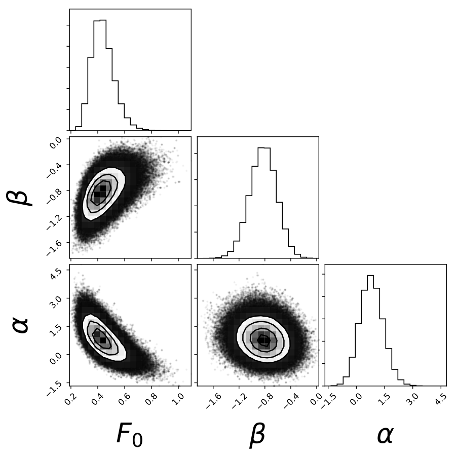
Figure 26 and Table 1 show and , as well as , with and without accounting for reliability, evaluated over all posterior values of . We see that even though there is significant overlap in the distributions with and without reliability, accounting for reliability has a strong impact: and are are reduced by more than 50%, which can be understood from the very small number of low-reliability planets in the region in Figure 24. is the integrated rate over a region of higher reliability, but reliability still has a strong effect. is the integrated rate over our entire period-radius analysis range, but it is dominated by the fact that there are more high-reliability planet candidates, so reliability has an impact similar to . Table 1 also shows the impact of accounting only for false alarm reliability, ignoring astrophysical false positive reliability, indicating that false alarm reliability accounts for about half the impact of the reliability correction.
We also computed occurrence for the SAG13 definition of 1010 10 https://exoplanets.nasa.gov/exep/exopag/sag/#sag13, days and . Without accounting for reliability, we find , consistent with the results of Zink & Hansen 2019, while accounting for reliability yields . This result should be treated with caution because it involves extrapolation beyond the domain of both reliability and detection completeness characterization.
We find that the impact of accounting for reliability is significant for small planets in long-period orbits. While one can note that the median values of occurrence rates in this regime are not much more than “one ” apart, the observed shifts in the distributions on the order of 40% are systematic, and clearly not due to statistical fluctuations.
VI.3 Simple Estimates of the Impact of Input Uncertainty
A full treatment of uncertainties in occurrence rates is beyond the scope of this paper. Uncertainties in stellar properties would need to be accounted for in the selection of the parent stellar population, the modeling behind the detection completeness and impact on the Robovetter. In this work we do, however, produce uncertainties in the false alarm reliability in §V.1 through the MCMC posteriors of the fit functions, as well as planet radius uncertainties that follow from stellar radius transit fit uncertainties as described in §III.2. In this section we present simple experiments that examine the impact on our occurrence rates of the reliability and planet radius uncertainties. We study the impact of planet radius uncertainties separately from the impact of reliability uncertainty.
VI.3.1 Impact of Planet Radius Uncertainty
We study the impact of planet radius uncertainties without accounting for reliability. We proceed in the same way that we study the impact of reliability, by performing several inference runs with a planet population in each run selected after applying the planet radius uncertainties. Specifically, for each run, prior to the restriction of the planet candidate population to the radius range , we add to each planet’s radius an error given by a draw from a Gaussian distribution with width equal to that planet’s radius uncertainty. Each planet is randomly assigned an upper or lower errorbar with 50% probability. The planet candidate population is then restricted to the range , and the inference is run.
| Parameter | No Uncertainty | Planet Radius Uncertainty |
|---|---|---|
The impact of planet radius uncertainties resulting from 1000 inference runs is shown in Table 2 and the top row of Figure 28. We see a small, consistent broadening of the width of the distributions and resulting error bars, and possibly a small systematic shift towards higher occurrence rates, but the overall impact is minor. We believe this is due to the smaller uncertainties resulting from using Gaia stellar properties, and from the fact that near the boundary of our planet size range there are many planets, so planets are equally likely to exit and enter our range due to uncertainty.
VI.3.2 Impact of Reliability Uncertainty
| Parameter | No Uncertainty | Reliability Uncertainty |
|---|---|---|
We study the impact of uncertainties in reliability by modifying the method of computing occurrence rates with uncertainty described in §VI.2. Prior to each inference run, we draw from the posteriors of the parameter vectors for false alarm efficiency (§V.1.1) and the observed false alarm rate (§V.1.2). We use these draws evaluate the FA efficiency and observed rate functions at each planet candidate’s period and observed MES, from which the false alarm reliability is computed. The reliability is then computed as described in §V.3, and each planet is included in that run with probability given by this computed reliability. In other words, the reliability rate function is realized for each run and applied to the planet candidate population.
Table 3 and the bottom row of Figures 28 compare occurrence rates with reliability correction but no reliability uncertainty, computed with the median of §V.1.1 and §V.1.2, with the reliability distribution that results from using the respective full posterior distributions. We see that there is no significant impact due to reliability uncertainty apparent in 1000 inference runs. This is in spite of the broad distributions of the low-reliability planet candidates shown in Figure 29, which shows the false alarm reliability values resulting from the posterior distributions. We believe this lack of impact on occurrence rates is due to the very small uncertainties for high-reliability targets (see Figure 23) combined with the facts that the low-reliability targets occur with less frequency in each inference and that most distributions in Figure 29 are close to symmetric, so are well-represented by their medians.
VI.4 Variations
In this section we explore the impact of changing some of the inputs and assumptions in the baseline occurrence rate computed in §VI.2. Our motivation is to understand the dependencies of the occurrence rate on these inputs and assumptions. In all cases except §VI.4.2 the same models were found to be the best fit to vetting completeness, false alarm effectiveness and observed false alarm rate as in the baseline case, though the parameters of these models had different values for the different variations.
We present the resulting variation in occurrence rates in Table 4, which includes results from Table 1 for comparison. This comparison is shown graphically for and at the end of this section in Figure 32.
VI.4.1 Using the Q1-Q17 DR25 Stellar Properties
Our baseline occurrence rates are substantially lower than several occurrence rates based on pre-Gaia stellar properties. In this section we repeat our analysis, replacing the Gaia-based catalog of Berger et al. 2020 with the pre-Gaia Q1-Q17 DR25 stellar properties from the NASA Exoplanet Archive4. We perform the same cuts as described in §III.1, with the exception that there is no cut on binary or evolved flags (these do not exist in the Q1-Q17 DR25 stellar properties) and we remove all stars with radius . The final catalog contains 75,541 GK stars.
We perform the same analysis as in the baseline case, starting from computing the vetting completeness for this stellar catalog, computing the summed completeness function , the reliability and occurrence rates specified in §VI.2. Figure 30 shows the resulting planet population, summed completeness and reliability. Comparison with Figure 24 shows that this catalog has more planet candidates in our period-radius range than when using Berger et al. 2020. This results in the higher occurrence rates shown in the “DR25” case in Table 4.
The choice of catalog has a stronger impact on than on : When not correcting for reliability, based on the DR25 stellar properties are about 15% higher than our baseline using Berger et al. 2020, while the DR25-based is about 60% higher. When correcting for reliability, based on the DR25 stellar properties are about 20% higher, while the DR25-based is 80% higher. Computing the SAG13 definition of 10using the DR25 stellar properties without correcting for reliability yields , while correcting for reliability gives .
The Berger et al. 2020 stellar catalog used in our baseline occurrence rates differs from the DR25 stellar catalog used in this section in both the values of the stellar properties themselves and in the cuts used to define the stellar parent population. In Appendix C we study the relative impact of the difference in stellar properties vs. the impact of the different population cuts on the difference in occurrence rates. We find that the difference in occurrence rates is primarily due to the different stellar properties, primarily stellar radius and effective temperature (leading to different GK selections), and that the differing population cuts have a minor impact.

VI.4.2 Baseline with a Score Cut of 0.9
The Robovetter outputs a score for each TCE, indicating the confidence with which the Robovetter vetted that TCE (Thompson et al. 2018). This score is not equivalent to reliability: for example the Robovetter confidently vetted several TCEs in the inverted/scrambled data incorrectly as PC with scores as high as 0.923. But score is roughly correlated with reliability, and Thompson et al. 2018 suggests computing high-reliability occurrence rates by considering only planet candidates with Robovetter score above some threshold. This will result in a smaller planet candidate population with lower completeness, but the resulting larger completeness correction will, in principle, correct the occurrence rate.
In this variation we impose an aggressive score cut, rejecting any planet candidate with score . We use the Berger et al. 2020 catalog, and compute the completeness and reliability as in the baseline case, treating any TCE with score as a false positive/alarm. Mulders et al. 2018 uses this score cut in their analysis, but their analysis is on a very different period-radius range so is not directly comparable to our results.

The result is a smaller, higher reliability planet candidate population, as shown in Figure 31, with noticeably lower completeness (compare the contours in Figure 24). In this case the false alarm vetting efficiency was best fit with the constant , resulting in a false alarm reliability very close to 1 for the entire period-radius range. The few planet candidates with lower reliability in Figure 31 are due to their astrophysical false positive probability, which results in and being slightly suppressed as shown in the “Score ” case in Table 4. This is an illustration of the fact that score cuts cannot be relied on to provide a population that is high reliability with respect to astrophysical false positives.
The agreement in when using this score cut and the baseline given in Table 1 is remarkable given the lack of planet candidates smaller than and orbital period days shown in Figure 31 (compare Figure 24). We interpret this agreement as an indication that the baseline is dominated by extrapolation because, in the baseline population, long-period, small planets have low reliability, as discussed in §VI.2. Because the baseline results and those using requiring score are essentially unconstrained extrapolations from radius and orbital period days to smaller planets and longer periods, we believe it is premature to conclude that using this score cut provides accurate occurrence rates for radius and orbital period days. In §VII we propose a strategy to explore this question.
VI.4.3 Baseline Without Vetting Completeness
This variation measures the impact of not including vetting completeness. This will result in a smaller completeness correction where vetting completeness is low, so we expect somewhat lower long-period, small planet occurrence rates. The “No Vetting Efficiency” case in Table 4 shows a small suppression in , and when not accounting for vetting completeness.
VI.4.4 Baseline Without MES Smearing
This variation measures the impact of not smearing the MES in the calculation of detection completeness, described in §IV.1. The “No MES Smear” case in Table 4 indicates an increase in small-planet, long-period occurrence rates measured by increases in and , but not smearing the MES has essentially no impact on .
| Case | No Reliability | With Reliability | No Reliability | With Reliability | No Reliability | With Reliability |
|---|---|---|---|---|---|---|
| Baseline (from Table 1) | ||||||
| DR25 | ||||||
| Score | ||||||
| No Vetting Efficiency | ||||||
| No MES Smear | ||||||
| Case | No Reliability | With Reliability | No Reliability | With Reliability | No Reliability | With Reliability |
| Baseline (from Table 1) | ||||||
| DR25 | ||||||
| Score | ||||||
| No Vetting Efficiency | ||||||
| No MES Smear | ||||||
VII Discussion
In this paper we show that a proper characterization of vetting completeness and reliability is important, particularly near the detection limit. In particular, in §VI.2 we find that characterizing Kepler reliability and completeness can impact occurrence rates by more than a factor of two near Kepler’s detection limit (see Table 1). We introduce a new approach to characterizing vetting completeness and reliability for the Kepler DR25 planet candidate population. This approach casts the problem as one of binomial probabilities via parameterized rate functions fitted to the DR25 injection, inverted and scrambled data. We develop parameterized models of completeness (described in §IV), false alarm effectiveness (§V.1.1) and the observed false alarm rate (§V.1.2). The particular parametric models we choose are selected via the Akieke information criterion, which chooses the parametric model that maximizes the likelihood corrected for the number of model parameters (see Appendix A). We do not claim that our parametric models are the best or in any sense “true”, just that they are the best of the parametric models we considered, described in Table 5. But our best models do a good job of accounting for the data, and are robust against choices such as grid resolution.
We caution, however, that vetting completeness and false alarm reliability as defined in this paper are properties of the specific Robovetter metrics and vetting thresholds behind the DR25 planet candidate catalog, as well as our analysis method, rather than properties of the detections themselves. For example, a different choice of Robovetter metrics may increase completeness while decreasing reliability or vice versa. While a low reliability for a transit detection from the analysis in this paper is reason to be cautious about asserting that detection is due to a true planet, further analysis of Kepler data can potentially result in higher confidence that a transit signal is due to a true planet. For example, as described in §II, at least one major source of false alarms, rolling bands, is highly dependent on focal plane position (Van Cleve & Caldwell 2009; Cleve et al. 2009). Though some of the DR25 vetting metrics, such as skye (Thompson et al. 2018) are focal-plane dependent, the reliability analysis in this paper largely ignores focal plane dependence by averaging over the focal plane, and potentially underestimates the reliability of a detection in a focal plane position known to have a low occurrence of, for example, rolling bands. Pixel-level analysis of transit events beyond that used in DR25 may be useful in distinguishing false alarms due to statistical fluctuations and cosmic ray events. These observations can potentially be implemented as new Robovetter metrics, which could result in a higher-reliability, more complete planet candidate catalog.
The four years of Kepler’s observation of its primary field provides a data set unlikely to be excelled in the near future. Full exploitation of this data for understanding exoplanet populations is only partially complete. This paper is an attempt to fill in a significant step in that exploitation. We deliberately chose to limit the innovations in this paper to the characterization of and correction for completeness and reliability, and the use of the uniform Gaia-based stellar properties catalog of Berger et al. 2020. We show the impact of these innovations by computing occurrence rates using standard methods from Burke et al. 2015 in order to facilitate comparison with previous occurrence rates based on similar methods. The following discussion critically examines the assumptions underlying these occurrence rates, revealing weaknesses in both the DR25 catalog and the occurrence rate calculation method, and outlines some of the directions that we believe will prove fruitful in addressing these weaknesses.
VII.1 Assumptions Underlying the Baseline Occurrence Rate
We illustrate the impact of reliability by computing a variety of occurrence rates near the Kepler detection limit (see §VI). We chose our specific occurrence rate method, Bayesian inference using a dual power law population model in period and radius, because it is standard and well-understood. We believe that our occurrence rates provide high-confidence insight into what the DR25 planet candidate catalog tells us about the exoplanet population for the period and radius range of days and under the following assumptions:
- •
The parent stellar population is statistically well-described by Berger et al. 2020.
- •
Detection and vetting completeness in the injected data, along with the analysis described in §IV, capture the statistical behavior of detection and vetting completeness in the observed data.
- •
The false alarms in the inverted and scrambled data capture the statistical behavior of the false alarms in the observed data.
- •
The astrophysical false positives probability statistically captures the probability of astrophysical false positives in the planet candidates.
- •
Exoplanets are distributed according to a Poisson point process.
- •
Dependence of planet occurrence on period and radius is modeled by a product of power laws in period and radius.
We discuss each of these assumptions in turn.
The parent stellar population: As stated in §III.1, we choose the Berger et al. 2020 stellar properties because they are informed by Gaia radii and uniformly treat the stellar properties across the parent population. While detailed observations of individual stars may provide more accurate stellar properties for individual stars, our method requires statistically uniform analysis. This is provided by the isochrone fitting approach of Berger et al. 2020. Therefore we believe that this stellar catalog is very well suited to our analysis. We showed in §VI.4.1, however, that the occurrence rate depends critically on the stellar properties in the parent population. Inaccuracies, in particular biases in stellar radius estimates, can have a strong impact on occurrence rates.
Detection and vetting completeness: The injected data and analysis from §IV makes many assumptions. The detection completeness analysis makes several empirical approximations (described in Burke & Catanzarite 2017) that may not apply well to individual planet candidate host stars. As described in §III, some of our stellar and planet candidate population approaches the restrictions stated in Burke & Catanzarite 2017 with respect to transit duration. Because our occurrence rates include regions with very few planet candidates, it is possible that the detection completeness for long-period planets is not as well modeled as that for short-period planets. Regarding vetting completeness, we are assuming that the Robovetter vets the injected detections with the same statistical accuracy as real transiting planets in the observed data. While we have confidence in this assumption, it is possible that some true planet transit signals have properties not captured by injection which confound the Robovetter, such as asymmetric transit shapes due to non-zero eccentricity, transit timing variations, and out-of-transit flux variations.
False alarm characterization: As we discussed in §V, inverted and scrambled data is believed to statistically model three identified classes of false alarms: rolling bands, statistical fluctuations combined with cosmic ray-induced pixel events that conspire to imitate long-period small transiting planets and stellar variability. The evidence for this belief is that the distribution of detected TCEs in the inverted and scrambled data closely matches the clearly anomalous distribution of detections in the observed data centered on the Kepler orbital period (see Thompson et al. 2018), and tuning the Robovetter to eliminate this distribution from the PC population in the inverted and scrambled data also eliminates the anomalous distribution in the observed data. While using the inverted and scrambled data to model the false alarm population is clearly effective, there are likely other types of false alarms not represented by the inverted/scrambled data, though these seem to be a minor component compared to those represented by inverted/scrambled data. Such unmeasured false alarms would cause an overestimate of false alarm reliability.
Astrophysical false positive characterization: The false positive probabilities (Morton et al. 2016) are computed making strong assumptions about the lack of evidence for stellar multiplicity associated with the transit host star. While these false positive probabilities model stellar multiplicity as candidate hypotheses, the prior used in this model strongly assumes a lack of evidence for stellar multiplicity. As described in Hirsch et al. 2017 and Ciardi et al. 2015, there is evidence that a non-trivial fraction, possibly 20%, of Kepler target stars have unknown stellar companions. Such companions could cause an overestimate of the reliability of a subset of the PC population.
Poisson Likelihood: The use of the Poisson likelihood (Equation (11)) for the distribution of exoplanets is a standard choice, but may not be correct. For example, the assumption that the probability of different planets on the same star are independent of one another (an assumption behind Equation (11)) is almost certainly not correct, as indicated by existence of many packed exoplanet systems. There is also evidence that the detection of one planet on a star can prevent the detection of other planets on the same star (Zink et al. 2019). Likelihood-free methods, such as approximate Bayesian computation as applied to occurrence rates in Hsu et al. 2018 or the population sampling method used in Zink & Hansen 2019 may yield more accurate occurrence rates.
The power law population model: Evidence is mounting against the use of a simple product of power laws in period and radius when modeling exoplanet population statistics. This is already apparent in the top-left panel of Figure 27, where the power law is a poor fit to the observed planet population as a function of radius. This is likely due to the Fulton gap (Fulton et al. 2017), though the orbital periods in our analysis are somewhat longer than in Fulton’s analysis. Further, Petigura et al. 2018 presents evidence that host star metallicity is an important parameter in exoplanet population statistics. As pointed out by Hsu et al. 2018, model mis-specification is unlikely to lead to accurate results. Several authors have avoided the use of parameterized models in occurrence rate computations (for examples, see Foreman-Mackey et al. 2014; Hsu et al. 2018; Howard et al. 2012), which is likely to lead to more accurate occurrence rates.
We believe that whatever method of statistical analysis is applied to the planet candidate catalog, characterizing and correcting for vetting completeness and reliability is critical. In the long-period, small-planet regime we have shown that reliability can reduce occurrence rates by a factor of two. We expect that this will be the case regardless of the statistical method and model, because reliability is a property of the planet candidate catalog. The effect of vetting completeness is less dramatic in the DR25 planet candidate catalog (as opposed to detection completeness, which is very important), but should not be neglected. Other planet catalogs may increase vetting reliability at the expense of vetting completeness, in which case vetting completeness can be more significant.
For habitability studies, the common practice of grouping together a wide class of stars and computing occurrence rates as functions of period and radius is potentially misleading. For example, the large range of stellar luminosities in our GK population shown in Figure 3 means that not all stars share the same habitable zones expressed as orbital periods. But grouping such a wide class of stars is necessary to provide the required statistics due to the small number of long-period, small planet detections and the sparseness of false alarms described in §V.1.1. Occurrence rates computed as functions of insolation flux and planet radius for the same class of stars would provide the needed statistics, and are likely more informative for habitable exoplanet population studies. Recent improvements in stellar characterization of the parent stellar sample, represented by Berger et al. 2020, make insolation-flux based occurrence rates a viable alternative.
VII.2 Improving the Planet Candidate Catalog
The discussion in §VII.1 outlines the assumptions behind extracting our occurrence rate from the DR25 planet candidate catalog, and how those assumptions may fail. The DR25 catalog itself can likely be improved upon, particularly in the long-period small planet regime. There is evidence that several long-period, small radius detections were incorrectly classified as false positives: the Kepler False Positive Working Group (FPWG) (Bryson et al. 2015) has identified several TCEs vetted as false positive in DR25 that are viable planet candidates, identified with fpwg_disp_status = POSSIBLE PLANET in the Kepler certified false positive table at the NASA Exoplanet archive2. This is expected because the DR25 vetting process deliberately balanced statistical uniformity and accuracy for individual objects, which was required for the study in this paper but compromised accurate vetting for some objects. In principle, the lowered completeness resulting from mis-classifying true planets as false positives is corrected by characterizing vetting completeness. But in the long-period, small-planet regime there are very few, low-reliability detections and very large completeness corrections (see Figure 24), which is vulnerable to large errors due to small statistics.
Accurate characterization of completeness and reliability as developed in this paper opens an intriguing approach to addressing the problem of few detections at long period and small radius: planet candidate catalogs that have lower reliability and higher completeness. This would mitigate the small-statistics problem by providing more detections with a smaller completeness correction resulting in better statistical constraints on the extrapolations discussed in §VI.4.2. We recommend an exploration of Robovetter thresholds that increase the number of detections, lowering reliability and increasing completeness. The methods to measure reliability described in this paper are a crucial step towards being able to extract more accurate occurrence rates from such a catalog.
We believe that the reliability of the planet candidate catalog can be improved by the development of metrics beyond those described in Thompson et al. 2018. We provide two examples that may prove fruitful.
- •
As described above, different regions of the Kepler focal plane have different different false alarm characteristics, which can be leveraged to more accurately evaluate the likelihood that a transit signal is due to a false alarm.
- •
Pixel-level analysis can be developed beyond the DR25 vetting metrics, based on the expectation that false alarms are likely to be significantly different from star-like transit signals at the pixel level, particularly in difference images (Bryson et al. 2013).
We expect that such improved vetting metrics will address the small statistics problem by increasing the reliability of planet candidates near the detection limit, so they have stronger statistical weight in occurrence rate calculations.
Followup observation can potentially play a role in validating the reliability characterization developed in this paper. Ground- or space-based observations of a significant number of DR25 PCs, confirming them as planets or determining them to be false positives, could provide a ground truth of the number of PCs that are true planets. This ground truth can be used to independently compute the reliability of the DR25 PC population. We caution against using such followup observations to modify the planet candidate catalog, however, as that is likely to violate the uniformity assumptions behind the completeness correction.
VIII Conclusion
This paper presents a new, probabilistic approach to statistically characterizing the vetting completeness and reliability Kepler DR25 exoplanet catalog. Using a standard occurrence rate calculation, we demonstrated that correcting for reliability can have a significant impact on occurrence rates, particularly near the Kepler detection limit at orbital periods longer than 200 days and planet radius 1.5 R⊕. We also showed that the choice of stellar properties for the searched stellar sample has a significant effect on occurrence rates. The results in this paper were made possible by the uniform detection and vetting methods behind DR25 that lend themselves to statistical characterization. We believe that the results presented in this paper are directly applicable to other exoplanet surveys such as K2, TESS, and PLATO so long as they create their catalogs in a similarly uniform way and expend the effort to create test data sets that measure completeness and false positives.
Appendix A Vetting Completeness and Reliability Model Selection
We investigated a variety of models for vetting completeness (§IV.2), false alarm efficiency (§V.1.1) and observed false alarm rate (§V.1.2). We selected the models based largely on the lowest Akiake Information Criterion , where is the number of degrees of freedom in the model and is the likelihood of the model. When comparing two models with likelihoods and , the relatively likelihood of model 1 relative to model 2 is given by . The AIC criterion is not always successful, however, particularly when the model contains parameters that do not converge. In addition, the lowest AIC sometimes results in models that are obviously not physical. In such cases we made judgement calls when making the selections, as described below.
Details of each model’s analysis is found on the GitHub website3 in the directory GKbaseline/htmlArchive.
The models we considered are defined in Table 5. All models have as input orbital period , MES (either expected for vetting completeness, or observed for reliability) , orbital period range , MES range and a parameter vector . has different elements for different models. The function evaluations start with scaling the period and MES input to in order to facilitate rotations. This scaling is done for consistency even if there are no rotations in the model. In some models, rotations are applied using angles and from . If there is only one rotation angle in , then .
| (A1) |
Many of the functions are constructed from the logistic function defined in equation (4). We also use the broken power law and non-normalized two-dimensional Gaussian
| (A2) |
| Model Name | Model Definition | Description | |
|---|---|---|---|
| constant | Constant function | ||
| gaussian | Gaussian + background | ||
| dualBrokenPowerLaw | Broken power law in and | ||
| logisticY0 | Logistic | ||
| logisticY | Logistic + constant | ||
| rotatedLogisticY |
Rotated logistic
+ constant | ||
| rotatedLogisticX0 | Rotated logistic | ||
| rotatedLogisticX02 |
Rotated logistic
w/ shape parameter | ||
| rotatedLogisticX0+gaussian |
Rotated logistic
+ Gaussian | ||
| logisticX0xlogisticY0 | logistic times logistic | ||
| logisticX0xlogisticY02 |
logistic times logistic
w/ shape parameters | ||
| logisticX0xRotatedLogisticY0 | logistic times rotated logistic | ||
| logisticX0xRotatedLogisticY02 |
logistic times
rotated logistic w/ shape parameter | ||
| rotatedLogisticYXLogisticY | logistic times rotated logistic + constant | ||
| rotatedLogisticX0xlogisticY0 |
Rotated logistic
times rotated logistic | ||
| rotatedLogisticX0xlogisticY02 |
Rotated logistic
times rotated logistic w/ shape parameters | ||
| rotatedLogisticYXFixedLogisticY |
fixed logistic times
rotated logistic + constant |
A.1 Vetting Completeness Model Selection
The functions considered for fitting the observed vetting completeness rate in §IV.2 are given in Table 6, along with AIC values and relative likelihoods. We chose logisticX0xRotatedLogisticY0 because it had the highest relative likelihood, best convergence behavior, and appears to be a good fit to the data.
| Model Name | Median AIC | Minimum AIC | Relative Likelihood |
|---|---|---|---|
| logisticY0 | 2819.03 | 2819.03 | 2.68e-137 |
| dualBrokenPowerLaw | 2246.87 | 2245.45 | 4.70e-13 |
| logisticX0xlogisticY0 | 2223.80 | 2223.79 | 4.82e-08 |
| logisticX0xlogisticY02 | 2227.20 | 2226.76 | 8.78e-09 |
| logisticX0xRotatedLogisticY0 | 2190.10 | 2190.11 | 1.00 |
| logisticX0xRotatedLogisticY02 | 2190.06 | 2189.83 | 1.02 |
| rotatedLogisticX0xlogisticY0 | 2192.08 | 2192.11 | 0.372 |
| rotatedLogisticX0xlogisticY02 | 2193.69 | 2193.19 | 0.166 |
A.2 False Alarm Effectiveness Model Selection
The functions considered for fitting the observed false alarm effectiveness rate in §V.1.1 are given in Table 7, along with AIC values and relative likelihoods. We chose rotatedLogisticX0 because it has a high relative likelihood, had the fewest parameters, and gave the most reasonable convergence results compared with other high-likelihood models.
| Model Name | Median AIC | Minimum AIC | Relative Likelihood |
|---|---|---|---|
| rotatedLogisticX0 | 214.39 | 214.06 | 1 |
| rotatedLogisticX02 | 212.49 | 210.93 | 1.70 |
| constant | 270.55 | 270.55 | 6.35e-13 |
| dualBrokenPowerLaw | 250.08 | 244.08 | 1.77e-08 |
| gaussian | 247.10 | 243.48 | 7.87e-08 |
| rotatedLogisticX0xlogisticY0 | 220.44 | 220.08 | 4.84e-02 |
| rotatedLogisticX0+gaussian | 228.03 | 216.74 | 1.09e-03 |
| rotatedLogisticY | 215.80 | 212.36 | 2.35e-02 |
| rotatedLogisticYXLogisticY | 220.60 | 216.53 | 4.47e-02 |
| logisticY | 238.92 | 238.45 | 4.69e-06 |
| rotatedLogisticYXFixedLogisticY | 215.95 | 212.58 | 0.458 |
A.3 Observed False Alarm Rate Model Selection
The functions considered for fitting the observed false alarm rate in §V.1.2 are given in Table 8, along with AIC values and relative likelihoods. We chose rotatedLogisticX0 because it gave the most reasonable results compared with other high-relative-likelihood models. We rejected rotatedLogisticX02 because one of its parameters did not converge.
| Model Name | Median AIC | Minimum AIC | Relative Likelihood |
|---|---|---|---|
| rotatedLogisticX0 | 307.20 | 307.19 | 1.00 |
| rotatedLogisticX0xlogisticY0 | 313.20 | 310.49 | 4.98e-02 |
| dualBrokenPowerLaw | 396.48 | 394.01 | 4.10e-20 |
| rotatedLogisticX02 | 302.87 | 301.10 | 8.71 |
| rotatedLogisticX0xlogisticY02 | 310.98 | 303.80 | 0.151 |
| rotatedLogisticX0+gaussian | 307.02 | 305.55 | 1.10 |
Appendix B Derivation of the Likelihood from the Poisson Probability
We briefly summarize Bayesian inference using a Poisson likelihood. We will work in the period-radius parameter space.
If our planet population is described by a point process with a period and radius-dependent rate , then the probability that planets occur around an individual star in some region (say a grid cell) of period-radius space is
where
We now cover our entire period-radius range with a sufficiently fine regular grid with spacing and so that each grid cell centered at period and radius contains at most one planet. Then in cell
We now ask: what is the probability of a specific number of planets in each cell ? We assume that the probability of a planet in different cells are independent, so
| (B1) |
because the cover and are disjoint. Here is the number of grid cells and is the number of grid cells that contain a planet = the number of planet candidates. So the grid has disappeared, and we only need to evaluate at the planet locations and integrate the rate function over the entire domain.
We do not observe all the planets, however. We account for incompleteness, including geometric transit probability, by replacing with in equation (B1), where is the completeness function for this star measured in §IV. The result is the probability
| (B2) |
We now consider the probability of detecting planets around a set of stars. Assuming that the planet detections on different stars are independent of each other, then the joint probability of a specific set of detections specified by the set in cell on on all stars indexed by is given by
| (B3) |
where and is the sum of the completeness functions over all stars.
We now let the rate function depend on a parameter vector , and consider the problem of finding the that maximizes the likelihood
| (B4) |
Because we are maximizing with respect to , we can ignore all terms that do not depend on . Therefore maximizing equation (B4) is equivalent to maximizing
| (B5) |
Appendix C Comparison of Catalog Cuts
In §VI.4.1 we found that using the DR25 stellar properties catalog results in larger occurrence ratse than the baseline of §VI.2, which uses the stellar properties from Berger et al. 2020. This difference can result from both the difference in the stellar properties themselves, and the fact that different stellar population cuts were used. In particular, as described in §III.1, the Berger et al. 2020 catalog contains only stars with good Gaia noise characteristics, and we impose further Gaia fit quality requirements by removing stars with qualityFlag = highRUWE.
In this appendix we explore the relative impact of the difference in stellar properties between the two catalogs compared with the impact of the different cuts. We consider the Berger et al. 2020 catalog with and without the cuts specific to this catalog. We then consider the same stars as Berger et al. 2020, but using the DR25 stellar properties and cuts. Finally we consider the DR25 stellar catalog and its restriction to those stars contained in the supplemental catalog of Mathur & Huber 2016. In all cases all steps of the occurrence rate computation are recomputed, including detection/vetting completeness and reliability.
We compute the occurrence rates and , defined in §VI. For two cases using the stellar properties of Berger et al. 2020 which differ in the population cuts:
- •
Case 1: the baseline of §VI.2, starting with the Berger et al. 2020 catalog, with all the cuts described in §III.1, and planet radii corrected for Gaia stellar radii as described in §III.2. Starts with 186,548 stars and ends up with 58,974 GK stars after cuts.
- •
Case 2: Same as case 1, starting with the Berger et al. 2020 catalog, except without the highRUWE, Bin or Evol cuts described in §III.1, replacing these cuts with the cut on stellar radius removing stars with described in §VI.4.1. Starts with 186,548 stars, and ends up with 66,956 GK stars after cuts.
We examine three cases using the DR25 stellar properties, which differ in the population cuts:
- •
Case 3: The same cuts as case 2, starting with the Berger et al. 2020 catalog, except using DR25 stellar properties and original DR25 planet radii. Starts with 186,548 stars and ends up with 71,168 GK stars after cuts.
- •
Case 4: The DR25 stellar catalog as described in section 4.1 using original DR25 planet radii. Starts with 200,038 stars and ends up with 75,541 GK stars after cuts.
- •
Case 5: The DR25 stellar catalog as in case 4, restricted to those stars in Mathur & Huber 2016 and using original DR25 planet radii. Starts with 197,096 stars and ends up with 74,989 GK stars after cuts.
Cases 1 through 3 start with the same stars, and differ in the cuts and the use of Gaia-based vs. DR25 stellar properties.
The occurrence rates and for the various cases are given in Table 9 and shown in Figure 33. We see that using the same stellar properties gives similar occurrence rates, with a noticeable difference in occurrence rates computed using different stellar properties. Differing cuts using the same stellar properties apparently has a much smaller impact. We therefore conclude that stellar properties (including differences in GK classification due to differences in effective temperature) is the dominant cause of the different occurrence rates, and the population cuts play a minor role. In all cases correcting for reliability has a significant impact on .
| Case | No Reliability | With Reliability | No Reliability | With Reliability | No Reliability | With Reliability |
|---|---|---|---|---|---|---|
| 1 | ||||||
| 2 | ||||||
| 3 | ||||||
| 4 | ||||||
| 5 | ||||||
We can get some insight into the change in occurrence rates by examining the impact of stellar properties on the PC population in the parameter space days and . We examine the difference between case 2 and case 3 because these cases start with the same parent stellar population and apply the same cuts. In case 2 these cuts are applied using the Berger et al. 2020 stellar properties, while in case 3 these cuts are applied using the DR25 stellar properties. In case 2 there are 107 PCs in the period and radius range out of 67,306 stars in the parent GK population, which yields 0.666 per star after dividing by the average completeness of 0.00239. In case 3 there are 116 PCs out of 71,168 stars in the parent GK population, which yields 0.64 planets per star after dividing by the average completeness of 0.00255. These simple estimates are consistent with the values of found in Table 9. To understand the changes in and , we need to examine in more detail how the stellar properties effect the PC population.
There are three ways that a difference in stellar properties can change the occurrence rate:
- •
A change in stellar radius causes a change in planet radius, which will impact the period-radius dependence of the population rate function and may cause the planet to move into or out of the range.
- •
A change in stellar radius causes the star to be added to or removed from the parent population depending on whether the star becomes smaller or larger than the cut.
- •
A change in stellar effective temperature causes the star to be added to or removed from the parent population because it is reclassified as GK or not GK.
Figure 34 shows the change in planet radius when changing from case 3 (DR25 stellar properties) to case 2, for those planet candidates that are common to both case 2 and case 3. We see that for periods between 50 and 200 days planet candidates both increase and decrease in size. For periods greater than 200 days, however, there is clear bias towards larger sizes. This effect is quantified by computing the average relative change in size in three period bins. The shortest period bin shows a near-zero average change in size, while the longest-period bin shows an average increase in size of about 8%, which is about a change.
Figure 35 shows planet candidates that either exited or entered the radius range considered in our occurrence rate in the change from case 3 to case 2. As in Figure 34, we see that at low period several planet candidates entered our planet radius domain of while other planet candidates left that domain. But for longer period, particularly days, planets left our domain by becoming too large while no planets entered our domain. Thus there is a loss of small exoplanets due to their being larger using Berger et al. 2020 stellar properties. In addition, several stars exited or entered our parent population through reclassification due to change in effective temperature.
These figures suggest that the change in planet size when using the Berger et al. 2020 stellar properties (case 2) is a significant contributing factor in the reduced occurrence rates. But it would not be correct to conclude that this change in planet size is the “cause” of the lower occurrence rate: changes in the parent stellar population also impact occurrence rates through changes in detection completeness and changes in population due to stellar reclassification and which stars pass the stellar size cut. It is only through computing the full occurrence rate that we can measure the impact of the stellar properties.
References
- Berger et al. (2018) Berger, T. A., Huber, D., Gaidos, E., & van Saders, J. L. 2018, ApJ, 866, 99
- Berger et al. (2020) Berger, T. A., Huber, D., van Saders, J. L., et al. 2020, arXiv e-prints, arXiv:2001.07737
- Borucki et al. (2010) Borucki, W. J., Koch, D., Basri, G., et al. 2010, Science, 327, 977
- Borucki et al. (2011) Borucki, W. J., Koch, D. G., Basri, G., et al. 2011, Astrophysical Journal, 736, 19
- Bryson et al. (2013) Bryson, S. T., Jenkins, J. M., Gilliland, R. L., et al. 2013, PASP, 125, 889
- Bryson et al. (2015) Bryson, S. T., Abdul-Masih, M., Batalha, N., et al. 2015, NExScI Exoplanet Archive, KSCI-19093-002
- Burke & Catanzarite (2017) Burke, C. J., & Catanzarite, J. 2017, NExScI Exoplanet Archive, KSCI-19111-002
- Burke et al. (2019) Burke, C. J., Mullally, F., Thompson, S. E., Coughlin, J. L., & Rowe, J. F. 2019, AJ, 157, 143
- Burke et al. (2015) Burke, C. J., Christiansen, J. L., Mullally, F., et al. 2015, Astrophysical Journal, 809, 8
- Caldwell et al. (2010) Caldwell, D. A., Kolodziejczak, J. J., Van Cleve, J. E., et al. 2010, Astrophysical Journal Letters, 713, L92
- Christiansen (2017) Christiansen, J. L. 2017, NExScI Exoplanet Archive, KSCI-19110-001
- Christiansen et al. (2013) Christiansen, J. L., Clarke, B. D., Burke, C. J., et al. 2013, Astrophysical Journal Supplement, 207, 35
- Christiansen et al. (2015) —. 2015, Astrophysical Journal, 810, 95
- Christiansen et al. (2016) —. 2016, Astrophysical Journal, 828, 99
- Ciardi et al. (2015) Ciardi, D. R., Beichman, C. A., Horch, E. P., & Howell, S. B. 2015, Astrophysical Journal, 805, 16
- Claret & Bloemen (2011) Claret, A., & Bloemen, S. 2011, A&A, 529, A75
- Cleve et al. (2009) Cleve, J. E. V., Christiansen, J. L., Jenkins, J. M., et al. 2009, MAST Archive, KSCI-19040-005
- Coughlin (2017) Coughlin, J. L. 2017, Planet Detection Metrics: Robovetter Completeness and Effectiveness for Data Release 25, Tech. rep.
- Coughlin et al. (2014) Coughlin, J. L., Thompson, S. E., Bryson, S. T., et al. 2014, AJ, 147, 119
- Dressing & Charbonneau (2015) Dressing, C. D., & Charbonneau, D. 2015, Astrophysical Journal, 807, 45
- Farr et al. (2014) Farr, W. M., Mandel, I., Aldridge, C., & Stroud, K. 2014, ArXiv astro-ph.EP/1412.4849
- Foreman-Mackey et al. (2013) Foreman-Mackey, D., Hogg, D. W., Lang, D., & Goodman, J. 2013, PASP, 125, 306
- Foreman-Mackey et al. (2014) Foreman-Mackey, D., Hogg, D. W., & Morton, T. D. 2014, Astrophysical Journal, 795, 64
- Fressin et al. (2013) Fressin, F., Torres, G., Charbonneau, D., et al. 2013, The Astrophysical Journal, 766, 81
- Fulton et al. (2017) Fulton, B. J., Petigura, E. A., Howard, A. W., et al. 2017, ArXiv e-prints, arXiv:1703.10375
- Hirsch et al. (2017) Hirsch, L. A., Ciardi, D. R., Howard, A. W., et al. 2017, Astronomical Journal, 153, 117
- Howard et al. (2012) Howard, A. W., Marcy, G. W., Bryson, S. T., et al. 2012, Astrophysical Journal Supplements, 201, 15
- Hsu et al. (2018) Hsu, D. C., Ford, E. B., Ragozzine, D., & Morehead, R. C. 2018, Astronomical Journal, 155, 205
- Jenkins (2002) Jenkins, J. M. 2002, ApJ, 575, 493
- Kirk et al. (2016) Kirk, B., Conroy, K., Prša, A., et al. 2016, Astronomical Journal, 151, 68
- Koch et al. (2010) Koch, D. G., Borucki, W. J., Basri, G., et al. 2010, ApJ, 713, L79
- Kraus et al. (in prep) Kraus, A., et al. in prep
- Lindegren (2018) Lindegren, L. 2018, gAIA-C3-TN-LU-LL-124
- Lindegren et al. (2018) Lindegren, L., Hernández, J., Bombrun, A., et al. 2018, A&A, 616, A2
- Mathur & Huber (2016) Mathur, S., & Huber, D. 2016, Kepler Science Document, KSCI-19097-004, Edited by Michael R. Haas and Natalie Batalha, 8
- Mathur et al. (2017) Mathur, S., Huber, D., Batalha, N. M., et al. 2017, ApJS, 229, 30
- Morton et al. (2016) Morton, T. D., Bryson, S. T., Coughlin, J. L., et al. 2016, Astrophysical Journal, 822, 86
- Morton & Johnson (2011) Morton, T. D., & Johnson, J. A. 2011, Astrophysical Journal, 738, 170
- Morton & Swift (2014) Morton, T. D., & Swift, J. 2014, Astrophysical Journal, 791, 10
- Mulders et al. (2018) Mulders, G. D., Pascucci, I., Apai, D., & Ciesla, F. J. 2018, AJ, 156, 24
- Pecaut & Mamajek (2013) Pecaut, M. J., & Mamajek, E. E. 2013, ApJS, 208, 9
- Petigura et al. (2013) Petigura, E. A., Howard, A. W., & Marcy, G. W. 2013, Proceedings of the National Academy of Science, 110, 19273
- Petigura et al. (2018) Petigura, E. A., Marcy, G. W., Winn, J. N., et al. 2018, AJ, 155, 89
- Santerne et al. (2012) Santerne, A., Díaz, R. F., Moutou, C., et al. 2012, Astronomy and Astrophysics, 545, A76
- Thompson et al. (2018) Thompson, S. E., Coughlin, J. L., Hoffman, K., et al. 2018, Astrophysical Journal Supplement, 235, 38
- Twicken et al. (2016) Twicken, J. D., Jenkins, J. M., Seader, S. E., et al. 2016, Astrophysical Journal, 152, 158
- Van Cleve & Caldwell (2009) Van Cleve, J. E., & Caldwell, D. A. 2009, MAST Archive, KSCI-19033-001
- Youdin (2011) Youdin, A. N. 2011, Astrophysical Journal, 742, 38
- Zink et al. (2019) Zink, J. K., Christiansen, J. L., & Hansen, B. M. S. 2019, MNRAS, 483, 4479
- Zink & Hansen (2019) Zink, J. K., & Hansen, B. M. S. 2019, MNRAS, 487, 246