A Top-Down Approach for the Multiple Exercises and Valuation of Employee Stock Options
Abstract
We propose a new framework to value employee stock options (ESOs) that captures multiple exercises of different quantities over time. We also model the ESO holder’s job termination risk and incorporate its impact on the payoffs of both vested and unvested ESOs. Numerical methods based on Fourier transform and finite differences are developed and implemented to solve the associated systems of PDEs. In addition, we introduce a new valuation method based on maturity randomization that yields analytic formulae for vested and unvested ESO costs. We examine the cost impact of job termination risk, exercise intensity, and various contractual features.
1 Introduction
The use of employee stock options (ESOs) as part of compensation is a common practice among large and small companies in the United States. Financial Accounting Standards Board (FASB) requires companies to value these stock options and report the total granting cost.11 1 See FASB Accounting Standards Codification (ASC) no.718 (formerly, FASB Statement 123R), Accounting for Stock-Based Compensation. This requirement raises the need for valuation methods that can effectively capture the payoff structure and exercise pattern of these stock options.
Empirical studies suggest that ESO holders tend to start exercising their options exercise early, often soon after the vesting period, and gradually exercise the remaining options over multiple dates before maturity. Huddart and Lang 1996, Marquardt 2002, and Bettis et al. 2005 point out that, for ESOs with 10 years to maturity, the expected time to exercise is 4 to 5 years. Investigating how ESO exercises are spread out over time, Huddart and Lang 1996 show that the mean fraction of options exercised by a typical employee at one time varied from 0.18 to 0.72. For more empirial studies, we refer to Huddart and Lang 1996, Bettis et al. 2001, Marquardt 2002, Armstrong et al. 2007, Hallock and Olson 2007, Heron and Lie 2016 and Carpenter et al. 2017. These empirical findings motivate us to consider a valuation model that account for multiple exercises of various units of options at different times. As noted by Jain and Subramanian 2004, “the incorporation of multiple-date exercise has important economic and account consequences.”
In this paper, we take the firm’s perspective to determine the cost of an ESO grant. An ESO grant commonly involves multiple options with a long maturity. There is also a vesting period, during which option exercise is prohibited and job termination leads to forfeiture of the options. The key component of our proposed valuation framework is an exogenous jump process that models the random exercises over time. Within our framework, the employee’s exercise intensity can be constant or stochastic, and the number of options exercised at each time can be specified to be deterministic or random. In essence, this top-down approach offers a flexible setup to model any exercise pattern. The idea is akin to the top-down approach in credit risk (Giesecke and Goldberg 2011), where the exogenous jump process represents portfolio losses. Since the ESO payoff depends heavily on when the employee leaves the firm, we also include a random job termination time and allow the job termination rate to be different during and after vesting period.
The valuation problem leads to the study of the system of partial differential equations (PDEs) associated with the vested and unvested options. In order to compute the ESO costs, we present two numerical methods to solve the PDEs. We discuss the method of fast Fourier transform (FFT), followed by the finite difference method (FDM). By applying Fourier transform, we simplify the original second-order PDEs to ODEs in the constant intensity case and first-order PDEs in the stochastic intensity case. The ESO costs are recovered via inverse fast Fourier transform. The results from the two methods are illustrated and compared under both deterministic and stochastic exercise intensities. Furthermore, we introduce a new valuation method based on maturity randomization. The key advantage of this method is that it yields analytic formulae, allowing for instant computation.
Using all three numerical methods, we compute the costs and examine the impact of job termination risk, exercise intensity, vesting period, and other features. Among our findings, we illustrate the distributions of exercise times under different model specifications, and also show that the average time of exercises tends to increase nonlinearly with the number of ESOs granted, resulting in a higher per-unit cost. In other words, under the assumption that the ESOs will be exercised gradually, a larger ESO grant has an indirect effect of delaying exercises, and thus leading to higher ESO costs.
In the literature, there are three main approaches for risk-neutral valuation and expensing of ESOs. Models are often be differentiated by their assumptions on exercise timing. One approach is to pre-specify an exercise boundary that determines the employee’s exercise strategy of a single ESO. In turn, the ESO is then priced as an option of barrier type (Hull and White 2004; Cvitanić et al. 2008). The boundary is typically chosen to be explicit and simple for the ease of computation but does not come with empirical or behavioral justification.
Another approach is to an optimal exercise time that maximizes the expected discounted payoff under some risk-neutral pricing measure (Leung and Wan 2015). Instead of the risk neutrality assumption, a number of related studies incorporate the employee’s risk preferences and hedging constraints and derive the optimal exercise strategy by solving a utility maximization problem. For this line of research, we refer to Jain and Subramanian 2004; Grasselli and Henderson 2009; Leung and Sircar 2009a; Leung and Sircar 2009b, and Carmona et al. 2011. In particular, Jain and Subramanian 2004 and Leung and Sircar 2009a, respectively, propose discrete-time and continuous-time models that allow the risk-averse employee to strategically exercise the ESOs over time rather than all on the same date. In addition to accounting for multiple-date exercises, Grasselli and Henderson 2009 also show that a risk-averse employee may find it optimal to exercise multiple options simultaneously at different exercise times.
In reality, firms do not know when ESOs will be exercised. Therefore, it is reasonable to model ESO exercises as some exogenous events so that the firm is not assumed to have access to the employee’s risk preferences and exercise strategy. This leads to the approach, as studied by Jennergren and Naslund 1993; Carr and Linetsky 2000 among others, that models ESO exercise by the first arrival time of an exogenous jump process. Although the exercises are exogenous events, the frequency and timing of their exercises can be dependent on the firm’s stock and other contractural features. Our proposed approach is essentially an extension of this approach to modeling multiple ESO exercises over the life of the options.
The rest of the paper is organized as follows. In Section 2, we present our ESO valuation model. The numerical method is discussed in Section 3. In Section 4, we discuss the case with stochastic exercise intensity. Then in Section 5 we introduce a novel valuation method based on maturity randomization. Finally, concluding remarks are provided in Section 7.
2 ESO Valuation Model
We begin by describing the ESO payoff structure, and then introduce the stochastic model that captures various sources of randomness. The valuation of both vested and unvested ESOs is presented.
2.1 Payoff Structure
The ESO is an early exercisable call option written on the company stock with a long maturity ranging from 5 to 10 years. In order to maintain the incentive effect of ESOs, the company typically prohibits the ESO holder (employee) from exercising during a vesting period from the grant date. During the vesting period, which ranges from 1 to 5 years, the holder’s departure from the company, voluntarily or forced, will lead to forfeiture of the option, rending it worthless. We denote [) as the vesting period, and after the date the ESO is vested and free to be exercised until it expires at time . The ESO payoff at any time is , where is the firm’s stock price at time and is the strike price. Upon departure, the employee is supposed to exercise all the remaining options. Figure 1 shows all four payoff scenarios associated with an ESO.

2.2 Job Termination and Exercise Process
The employee’s job termination plays a crucial role in the exercise timing and resulting payoff of the ESOs. We model the job termination time during the vesting period by an exponential random variable , with . When the ESO becomes vested after , we model the employee’s job termination time by another exponential random variable , with . We assume that and are mutually independent. This approach of modeling job termination by an exogenous random variable is also used by Jennergren and Naslund 1993, Carpenter 1998, Carr and Linetsky 2000, Hull and White 2004, Sircar and Xiong 2007, Leung and Sircar 2009b, Carmona et al. 2011, and Leung and Wan 2015, among others. In our model, using two different exponential times allows us to account for the varying level of job termination risk during and after the vesting period.
An ESO grant typically contains multiple options. Empirical studies show that employee tends to exercise the options gradually over time, rather than exercising all options at once. This motivates us to model the sequential random timing of exercises. In our proposed model, we consider a grant of units of identical early exercisable ESOs with the same strike price and expiration date . These ESOs are exercisable only after the vesting period . For the vested ESOs, we define the random exercise process , for , to be the positive jump process representing the number of ESOs exercised over time. As such, is an integer process that takes value on . The corresponding jump times are denoted by the sequence , and the frequency of exercises is governed by the jump intensity process .
The jump size for the th jump of represents the number of ESOs exercised and is described by a discrete random variable . The exercise process starts at time with . By definition, we have . This means that the random jump size at any time must take value within . Also, as soon as reaches the upper bound , the jump intensity must be set to be zero thereafter. Given that the employee still holds options, the probability mass function of the random jump size is
| (1) |
In turn, the expected number of options to be exercised at each exercise time is given by
| (2) |
which again depends on the current number of ESOs held.
The employee may exercise single or multiple units of ESOs over time. On the date of expiration or job termination, any unexercised options must be exercised. Hence, the discounted payoff from the ESOs over is a sum of two terms, given by
| (3) |
The indicator means that the ESO payoff is zero if the employee leaves the firm during the vesting period.
Example 1 (Unit Exercises)
Suppose be a nonhomogeneous Poisson process with a time-varying jump intensity function , for . At each jump time a single option is exercised. In Figure 2 we illustrate three possible scenarios. In scenario (i), the employee exercises 6 out of 10 options one by one, but must exercise 4 remaining options upon job termination realized at time . In scenario (ii) the employee exercises all 10 options one by one before maturity. In scenario (iii), the employee has not exercised all the options by maturity, so all remaining options are exercised at time .

Example 2 (Block Exercises)
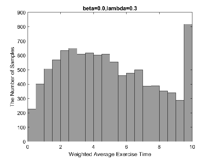
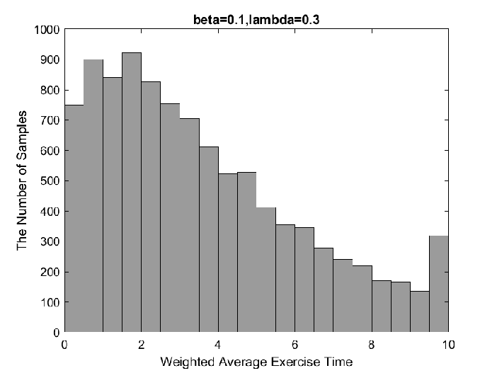
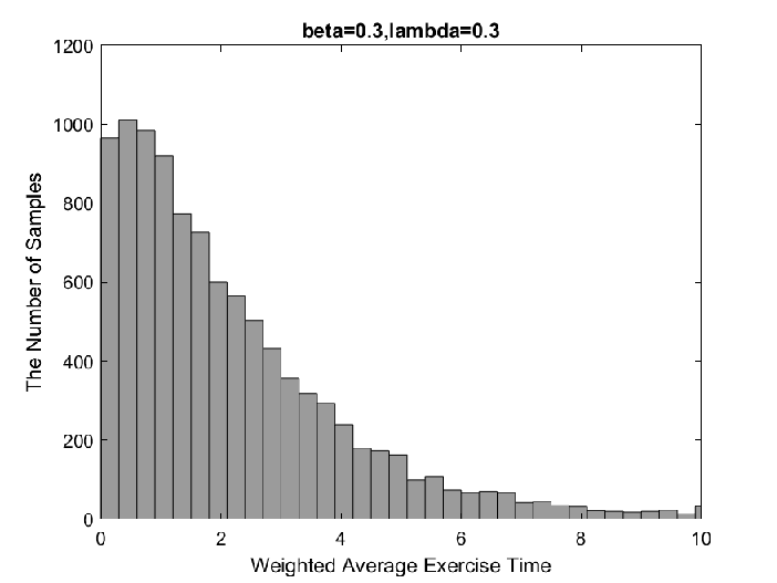
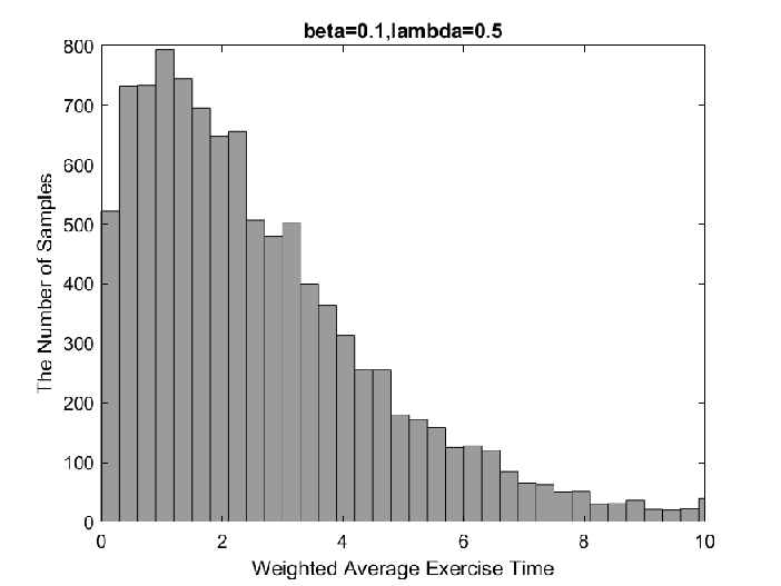
Suppose the employee can exercise one or more options at each exercise time. As an example, We assume a uniform distribution for the number of options to be exercised, so we set for . In Figure 3, we illustrate the distributions of the weighted average exercise time defined by
| (4) |
where is the number of ESOs exercised at the th exercise time , and is the number of distinct exercise times before or at time . For each simulated path, we take an average of the distinct exercise times weighted by the number of options exercised at each time. With common parameters , the histograms of correspond to different values of and . With a low job termination rate and low exercise intensity (panel (a) where , ), more options tend to be exercised at maturity. Comparing panel (b) to panel (c), and also panel (b) to panel (d), we see that a higher job termination rate or higher exercise intensity lowers the average exercise time and reduces instances of exercising at maturity. Similar patterns can also be found in empirical studies (Heron and Lie 2016, Fig. 3).
2.3 PDEs for ESO Valuation
To value ESOs, we consider a risk-neutral pricing measure for all stochastic processes and random variables in our model. We model the firm’s stock price process by a geometric Brownian motion
| (5) |
where the positive constants , and are the interest rate, dividend rate, and volatility parameter respectively, and is a standard Brownian motion under , independent of the exponentially-distributed job termination times and . Our default assumption for the employee’s exercise intensity is that it is a deterministic function of time, denoted by . We will discuss the case with a stochastic exercise intensity in Section 4.
At any time , the ESO is vested. The vested ESO cost functions , for , where is the number of options currently held, are given by the risk-neutral expectation of discounted future ESO payoffs provided that the employee has not left the firm.
| (6) |
for , and .
Next, we define the infinitesimal generator associated with the stock price process by
| (7) |
We determine the vested ESO costs by solving the following system of PDEs.
| (8) |
for and . Here, is the expected number of options exercised and is the probability of exercising options with options left. The terminal condition is for .
During the vesting period , the ESO is unvested and is subject to forfeiture if the employee leaves the firm. We denote the cost of units of unvested ESO by . Since holding an unvested ESO effectively entitles the holder to obtain a vested ESO at time provided the holder is still with the firm. If the ESO holder leaves the firm at any time , the unvested ESO cost is zero. Otherwise, given that , the (pre-departure) unvested ESO cost is
| (9) |
To determine the unvested ESO cost, we solve the PDE problem
| (10) | |||||
Here, is the vested ESO cost evaluated at time .
3 Numerical Methods and Implementation
In this section, we present two numerical methods to solve PDE (8). We first discuss the application of fast Fourier transform (FFT) to ESO valuation, followed by the finite difference method (FDM). The results from the two methods are compared in Section 3.3.
3.1 Fast Fourier Transform
We first consider the vested ESO (). Let such that , and define the function
| (11) |
for each . The PDE for is given by
| (12) |
where
| (13) |
The terminal condition is , for .
The Fourier transform of is defined by
| (14) |
for , with angular frequency in radians per second. Applying Fourier transform to PDE (12), we obtain an ODE for , a function of time parametrized by , for each . Precisely, we have
| (15) |
where
| (16) | ||||
| (17) | ||||
| (18) |
with the terminal condition . Solving the ODE, we obtain
| (19) |
Accordingly, we can recover the vested ESO cost function by inverse Fourier transform:
| (20) |
for every , and
In the literature, Leung and Wan 2015 apply a Fourier time-stepping (FST) method it to compute the cost of an American-style ESO when the company stock is driven by a Levy process. This FST method has been applied more broadly by Jackson et al. 2008 to solve partial-integro differential equations (PIDEs) that arise in options pricing problems.
Remark 3
For numerical implementation, we work with a finite domain with uniform discretization of lengths and in the time-space dimensions. We set , , and . Similarly, we discrete the finite frequency space with uniform grid size of , where we apply the Nyquist critical frequency that and . For , and , we denote , , and
| (26) |
Then we numerically compute the discrete Fourier transform
| (27) |
with . In (27), we evaluate the sum by applying the standard fast Fourier transform (FFT) algorithm. The corresponding Fourier inversion is conducted by inverse FFT, yielding the vested ESO cost . Note that the coefficient will be cancelled in the process.
As for the unvested ESO, we define the associated cost function
| (28) |
for each . From PDE (10), we derive the PDE for
| (29) |
for , with the terminal condition , for . As we can see, once the vested ESO cost is computed, it determines the terminal condition for the unvested ESO problem.
Applying Fourier transform to (29), we can derive the ODE for ,
| (30) |
where
| (31) |
for , with the terminal condition . We solve the ODE to get
| (32) |
In turn, we apply inverse Fourier transform to recover the unvested ESO cost:
| (33) |
for . Again, we apply FFT to numerically compute the Fourier transform and use inverse FFT to recover the cost function.
3.2 Finite Difference Method
For comparison, we also compute the ESO costs using a finite difference method. Specifically, we apply the Crank-Nicolson method on a uniform grid. Here we provide an outline with focus on the boundary conditions for our application. For more details, we refer to Wilmott et al. 1995, among other references.
As for grid settings, We restrict the domain to a finite domain , where must be relatively very large such that if the current stock price , then the stock price will be larger than the strike price over with great probability.
To determine the boundary condition at , we introduce a new function
for . When , we see that . Thus, we can set the boundary condition at to be . By Feynman-Kac formula, satisfies the PDE
| (34) |
for , and , with terminal condition , for . Then, has the ansatz solution
| (35) |
where and satisfy the pair of ODEs respectively,
| (36) | |||
for , and , with the terminal condition , for . We can solve the ODEs (36) analytically, or numerically solve it using the backward Euler method.
Next, we discrete the domain with uniform grid size of and . Then, we apply to denote discrete approximations of where and . The Crank-Nicolson method is applied to solve the PDEs satisfied by , for . Working backward in time, we obtain the vested ESO costs at time , which become the terminal condition values for the unvested ESO valuation problem. For the unvested ESO cost, we restrict the domain to the finite domain , where is relatively very large such that
| (37) | ||||
| (38) | ||||
| (39) |
We again apply the Crank-Nicolson method solve the PDEs satisfied by , for .
3.3 Numerical Examples
Using both FFT and FDM we compute different ESO costs by varying the vesting period , job termination rate and , as well as exercise intensity . In Table 1, we present the ESO costs and compare the two numerical methods. It is well known that the call option value is increasing with respect to its maturity. In a similar spirit if the employee tends to exercise the ESO earlier, then a smaller ESO cost is expected. As we can see in Table 1, the ESO cost decreases as exercise intensity increases, or as job termination rate or increases, holding other things constant. On the other hand, the effect of vesting period is not monotone. In a scenario with a high job termination during the vesting period, the employee is very likely to leave the firm while the options are unvested, leading to a zero payoff. Consequently, the ESO cost is decreasing with respect to . This corresponds to the case with in Table 1. However, if is small, then the employee is unlikely to leave the firm and lose the options during the vesting period. Therefore, a longer vesting period would effectively make the employee hold the options for a longer period of time, delaying the exercise. As a result, the ESO cost is increasing with respect to , which is shown in other cases in Table 1.
| Parameters | |||||||
|---|---|---|---|---|---|---|---|
| FDM | FFT | FDM | FFT | FDM | FFT | ||
| 5.4729 | 5.4753 | 7.8399 | 7.8405 | 8.2845 | 8.2849 | ||
| 3.7067 | 3.7101 | 6.9164 | 6.9170 | 7.7054 | 7.7058 | ||
| 3.2483 | 3.2522 | 6.7063 | 6.7069 | 7.5746 | 7.5750 | ||
| 2.7024 | 2.7069 | 6.4655 | 6.4661 | 7.4253 | 7.4257 | ||
| 5.0603 | 5.0629 | 9.3022 | 9.3031 | 12.1510 | 12.1517 | ||
| 3.5595 | 3.5630 | 8.3622 | 8.3631 | 11.4298 | 11.4306 | ||
| 5.0603 | 5.0629 | 1.2579 | 1.2590 | 0.2219 | 0.2226 | ||
| 3.5595 | 3.5630 | 1.1310 | 1.1318 | 0.2087 | 0.2094 | ||
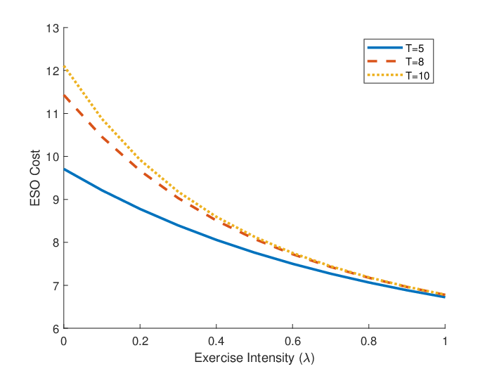
In Figure 4, we plot the ESO cost as a function of the exercise intensity for , 8 and 10. It shows that the ESO is decreasing and convex with respect to . An employee with a high exercise intensity tends to exercise the ESOs earlier than those with a lower exercise intensity. Since the call option value increases with maturity, exercising the ESO earlier will result in a lower cost. As the exercise intensity increases from zero, the ESO cost tends to decrease faster than when the exercise intensity is higher. Moreover, Figure 4 also shows that as increases, the ESO costs associated with different maturities , 8 and 10 get close to each other. The intuition is that when is large, the options will be exercised very early and the maturity will not have a significant impact on the option values.
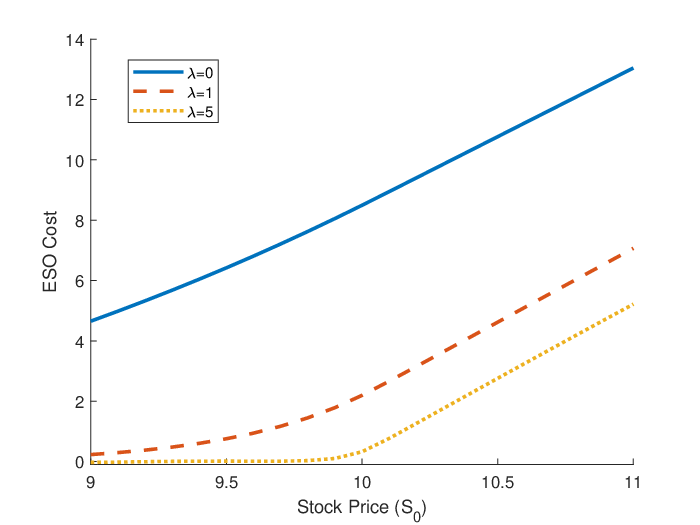
On the right panel of Figure 4, we plot the option value as a function of stock price with exercise intensity , 1 or . It shows that, as increases from 0 to 1, the option value decreases rapidly. When the exercise intensity is very high, i.e. in the figure, there is a high chance of immediate exercise, so the ESO value is seen to be very close to the ESO payoff .
Next, we consider the effect of the total number of ESOs granted. Intuitively we expect the total cost to increase as the number of options increases, but the effect is far from linear. In Figure 5 we see that the average per-unit cost and average time to exercise are increasing as increases. In other words, under the assumption that the ESOs will be exercised gradually, a larger ESO grant has an indirect effect of delaying exercises, and thus leading to higher ESO costs. The increasing trends hold for different exercise intensities, but the rate of increase diminishes significantly for large . Also, the higher the exercise intensity, the lower the per-unit cost and shorter averaged time to exercise.


4 Stochastic Exercise Intensity
Now we discuss the stochastic exercise intensity, an extension to the previous model, that , which is the function not only depends on the time also depends on the stock price . Accordingly, the corresponding vested ESO cost will satisfy
| (40) | ||||
for , and , with terminal condition , for .
Since we only discuss the stochastic exercise intensity and the employee will not exercise the option during the vesting period, the PDE for unvested ESO will remain unchanged. Next, we will discuss how to numerically solve (40) by FFT.
For applying Fourier transform, we use the same notation as in Section 3.1 that
| (41) |
for , , and
| (42) |
for . In this section, we assume that , for some positive time-dependent functions and . For implementation, we assume be relative small, such that stay positive in the truncated space . Then, satisfies
| (43) | ||||
where is defined in (13). The terminal condition is , for .
where
| (45) | ||||
| (46) |
for .
Observe that (44) is a first-order PDE with terminal condition that (see (18)). Therefore, we apply the method of characteristics and get
| (47) |
where
| (48) |
For numerical implementation, we can use the similar method mentioned in Section 3.1. We can make the approximation
| (49) |
where . The integral in (47) and (48) can be approximated similarly or computed explicitly depending on the choice of .
Table 2 presents the ESO costs in the cases of constant exercise intensity and stochastic intensity with under different vesting periods and job termination rates. The stochastic intensity specified here can be larger or smaller than the constant level 0.2 depending on whether the current stock price is higher or lower than the strike price . For each case, we compute the ESO cost using both FFT and FDM. For the latter, we apply the Crank-Nicolson method on a uniform grid and adopt Neumann condition at the boundary (see Section 3.2). As we can see, the costs from the two methods are practically the same. As the vesting period lengthens, from to , the ESO cost tends to increase under different exercise intensities and job termination rates. When the job termination rate is zero, the ESO costs with stochastic intensity appear to be higher, but this effect is greatly reduced as the job termination rate increases. This is intuitive since a high job termination rate means that most ESOs will be exercised or forfeited at the departure time, rather than exercised according to an exercise process over the life of the options.
| Parameters | |||||||
|---|---|---|---|---|---|---|---|
| FDM | FFT | FDM | FFT | FDM | FFT | ||
| 12.8052 | 12.8065 | 13.7122 | 13.7134 | 15.0953 | 15.0967 | ||
| 11.5867 | 11.5878 | 11.2266 | 11.2276 | 10.1187 | 10.1196 | ||
| 7.8849 | 7.8859 | 9.6380 | 9.6388 | 12.4022 | 12.4029 | ||
| 7.1347 | 7.1355 | 7.8910 | 7.8916 | 8.3135 | 8.3139 | ||
| 12.8310 | 12.8379 | 13.7364 | 13.7445 | 15.1130 | 15.1235 | ||
| 11.6099 | 11.6163 | 11.2464 | 11.2531 | 10.1305 | 10.1376 | ||
| 7.8895 | 7.8887 | 9.6428 | 9.6423 | 12.4068 | 12.4076 | ||
| 7.1387 | 7.1381 | 7.8948 | 7.8946 | 8.3165 | 8.3172 | ||
5 Maturity Randomization
In this section, we propose an alternative method to value ESOs. It is an analytical method that yields an approximation to the original ESO valuation problem discussed in Section 2.3. The core idea of this method is to randomize the ESO’s finite maturity by an exponential random variable , with where here is original constant maturity. Such a choice of parameter means that ; that is, the ESO is expected to expire at time . For instance, if the maturity of the ESOs is 10 years, then the randomized maturity is modeled by . Such a maturity randomization allows us to derive an explicit approximation for ESO cost.
5.1 Vested ESO
First we consider the ESO cost at the end of the vesting period. Provided that the employee remains at the firm by time , the vested ESO has a remaining maturity of length . Therefore, for the exponentially distributed maturity , one may set . At time , the vested ESO cost function is given by
| (50) | ||||
| (51) | ||||
| (52) |
for . From (52), we derive the associated ODE for . For the convenience, we denote
| (53) |
Then, we obtain a system of second-order linear ODEs:
| (54) |
for , and , with the boundary condition .
Proposition 4
Proof. We begin by considering the case that the employee only holds a single option. With , the general solution to ODE (54) is given by
| (58) |
where
| (59) |
By imposing that and to be continuous at the strike price , we consider at and obtain
In addition, since , we will have to guarantee that . And, when , the maturity , -a.s., which will lead to . Therefore, we have . As a result, we obtain the remaining non-zero coefficients:
| (70) |
For , the general solution to ODE (54) is
| (71) |
Applying ODE (54), we obtain the relationship between the coefficients of and the coefficients of , for , as follows:
| (72) |
for .
In addition, the continuity of and around strike price yields that
| (73) |
Rearranging, we obtain the remaining coefficients for the solution:
| (74) |
5.2 Unvested ESO
For the unvested ESO, we can model the vesting time by the exponential random variable , where . Then, the unvested ESO cost at time is given by
| (75) | ||||
| (76) |
Then we will can derive the ODE for :
| (77) | ||||
Assuming , we could derive the solution for from the solution for in (71), which is
| (78) |
where
| (79) |
and
| (80) |
with
| (81) |
Alternatively, one can use FDM or FFT to calculate the unvested ESO cost without applying maturity randomization for the second time.
In Figure 6, we show the cost of an unvested ESO, computed by our maturity randomization method, as a function of the initial stock price , along with the ESO payoff. As expected, the ESO cost is increasing convex in . Comparing the costs corresponding to two different job termination rates during the vesting period, we see that a higher job termination rate reduces the ESO value. This is intuitive as the employee has a higher chance of leaving the firm during the vesting period and in turn losing the option entirely.
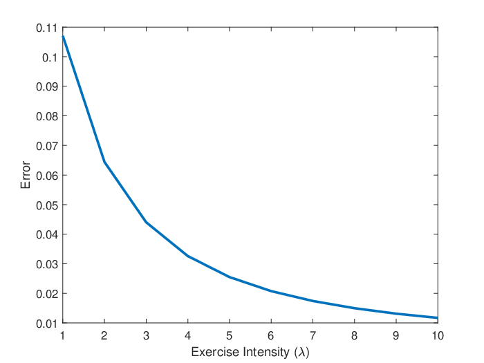
The maturity randomization method delivers an analytical approximation that allows for instant computation. In Figure 7, we examine errors of this method. As we can see, as the exercise intensity or post vesting job termination rate increases the valuation error decreases exponentially to less than a penny for each option. This shows that the maturity randomization method can be very accurate and effective for ESO valuation.


6 Implied Maturity
Given that ESOs are very likely to be exercised prior to expiration, the total cost of an ESO grant is determined by how long the employee effectively holds the options. For each grant of options, the exercise times are different and they depend on the valuation model and associated parameters. Therefore, we introduce the notion of implied maturity to give an intuitive measure of the effective maturity implied by any given valuation model.
Like the well-known concept of implied volatility, we use the Black-Scholes option pricing formula. The price of a European call with strike and maturity is given by
| (82) |
where
| (83) |
Next, recall the ESO cost function under the top-down valuation model in Section 2. Then, the implied maturity for ESOs is defined to be the maturity parameter such that
| (84) |
holds, with all other parameters held constant. To define implied maturity under another model only requires replacing the corresponding cost function on the right-hand side in (84).
Through the lens of implied maturity, we can see the model and parameter effects in terms of how long the employee will hold the option under the Black-Scholes model. For example, if the exercise intensity increases, then the ESOs are more likely to be exercised early, resulting in a lower cost. Since the call option value is increasing in maturity, the implied maturity is expected to decrease as exercise intensity increases. The plots in Figure 8 confirm this intuition. Moreover, under high exercise intensity all ESOs will be exercised very early and the contract maturity will play a lesser role on the ESO cost and thus implied maturity. Indeed, Figure 8 shows that implied maturities associated with different contract maturities and get closer to each other as increases.
Next, we consider the effect of the total number of ESOs granted. Intuitively we expect the implied maturity to increase as the number of options increases, but the effect is far from linear. In Figure 9, we see that the implied maturity is increasing as increases. In other words, under the assumption that the ESOs will be exercised gradually, a larger ESO grant has an indirect effect of delaying exercises, and thus leading to higher implied maturity. The increasing trends hold for different exercise intensities, but the rate of increase diminishes significantly for large . Also, the higher the exercise intensity, the lower the implied maturity.


7 Conclusion
We have studied a new valuation framework that allows the ESO holder to spread out the exercises of different quantities over time, rather than assuming that all options will be exercised at the same time. The holder’s multiple random exercises are modeled by an exogenous jump process. We illustrate the distribution of multiple-date exercises that are consistent with empirical evidence. Additional features included are job termination risk during and after the vesting period. For cost computation, we apply a fast Fourier transform method and finite difference method to solve the associated systems of PDEs. Moreover, we provide an alternative method based on maturity randomization for approximating the ESO cost. Its analytic formulae for vested and unvested ESO costs allow for instant computation. The proposed numerical method is not only applicable to expensing ESO grants as required by regulators, but also useful for understanding the combined effects of exercise intensity and job termination risk on the ESO cost. For future research, there are a number of directions related to our proposed framework. For many companies, risk estimation for large ESO pool is both practically important and challenging. Another related issue concerns the incentive effect and optimal design of ESOs so that the firm can better align the employee’s interest over a longer period of time.
References
- Armstrong et al. (2007) Armstrong, C. S., Jagolinzer, A. D., and Larcker, D. F. (2007). Timing of employee stock option exercises and the cost of stock option grants. Working paper, Stanford University.
- Bettis et al. (2001) Bettis, J. C., Bizjak, J. M., and Lemmon, M. L. (2001). Managerial ownership, incentive contracting, and the use of zero-cost collars and equity swaps by corporate insiders. Journal of Financial and Quantitative Analysis, 36:345–370.
- Bettis et al. (2005) Bettis, J. C., Bizjak, J. M., and Lemmon, M. L. (2005). Exercise behaviors, valuation, and the incentive effects of employee stock options. Journal of Financial Economics, 76(2):445–470.
- Carmona et al. (2011) Carmona, J., León, A., and Vaello-Sebastiá, A. (2011). Pricing executive stock option under employment shocks. Journal of Economic Dynamics and Control, 35:97–114.
- Carpenter (1998) Carpenter, J. (1998). The exercise and valuation of executive stock options. Journal of Financial Economics, 48:127–158.
- Carpenter et al. (2017) Carpenter, J. N., Stanton, R., and Wallace, N. (2017). Estimation of employee stock option exercise rates and firm cost. Working paper, New York University and U.C. Berkeley.
- Carr and Linetsky (2000) Carr, P. and Linetsky, V. (2000). The valuation of executive stock options in an intensity-based framework. European Finance Review, 4:211–230.
- Cvitanić et al. (2008) Cvitanić, J., Wiener, Z., and Zapatero, F. (2008). Analytic pricing of employee stock options. Review of Financial Studies, 21(2):683–724.
- Giesecke and Goldberg (2011) Giesecke, K. and Goldberg, L. (2011). A top down approach to multi-name credit. Operations Research, 59(22):283–300.
- Grasselli and Henderson (2009) Grasselli, M. and Henderson, V. (2009). Risk aversion and block exercise of executive stock options. Journal of Economic Dynamics and Control, 33(1):109–127.
- Hallock and Olson (2007) Hallock, K. and Olson, C. A. (2007). New data for answering old questions regarding employee stock options. In Abraham, K. G., Spletzer, J. R., and Harper, M., editors, Labor in the New Economy, pages 149 – 180. University of Chicago Press.
- Heron and Lie (2016) Heron, R. A. and Lie, E. (2016). Do stock options overcome managerial risk aversion? Evidence from exercises of executive stock options (ESOs). Management Science, 63(9):2773–3145.
- Huddart and Lang (1996) Huddart, S. and Lang, M. (1996). Employee stock option exercises: an empirical analysis. Journal of Accounting and Economics, 21:5–43.
- Hull and White (2004) Hull, J. and White, A. (2004). How to value employee stock options. Financial Analysts Journal, 60:114–119.
- Jackson et al. (2008) Jackson, K. R., Jaimungal, S., and Surkov, V. (2008). Fourier space time-stepping for option pricing with Lévy models. Journal of Computational Finance, 12(2):1–29.
- Jain and Subramanian (2004) Jain, A. and Subramanian, A. (2004). The intertemporal exercise and valuation of employee options. The Accounting Review, 79:705–743.
- Jennergren and Naslund (1993) Jennergren, L. and Naslund, B. (1993). A comment on ‘Valuation of stock options and the FASB proposal’. Accounting Review, 68:179–183.
- Leung and Sircar (2009a) Leung, T. and Sircar, R. (2009a). Accounting for risk aversion, vesting, job termination risk and multiple exercises in valuation of employee stock options. Mathematical Finance, 19(1):99–128.
- Leung and Sircar (2009b) Leung, T. and Sircar, R. (2009b). Exponential hedging with optimal stopping and application to ESO valuation. SIAM Journal of Control and Optimization, 48(3):1422–1451.
- Leung and Wan (2015) Leung, T. and Wan, H. (2015). ESO valuation with job termination risk and jumps in stock price. SIAM Journal on Financial Mathematics, 6(1):487–516.
- Marquardt (2002) Marquardt, C. (2002). The cost of employee stock option grants: an empirical analysis. Journal of Accounting Research, 4:1191–1217.
- Sircar and Xiong (2007) Sircar, R. and Xiong, W. (2007). A general framework for evaluating executive stock options. Journal of Economic Dynamics and Control, 31(7):2317–2349.
- Wilmott et al. (1995) Wilmott, P., Howison, S., and Dewynne, J. (1995). The Mathematics of Financial Derivatives. Cambridge University Press.