Adversarial Mahalanobis Distance-based Attentive Song Recommender for Automatic Playlist ContinuationConference: Proceedings of the 42nd International ACM SIGIR Conference on Research and Development in Information Retrieval; July 21–25, 2019; Paris, FranceProceedings of the 42nd International ACM SIGIR Conference on Research and Development in Information Retrieval (SIGIR ’19), July 21–25, 2019, Paris, FrancePrice: 15.00DOI: 10.1145/3331184.3331234ISBN: 978-1-4503-6172-9/19/07
Abstract.
In this paper, we aim to solve the automatic playlist continuation (APC) problem by modeling complex interactions among users, playlists, and songs using only their interaction data. Prior methods mainly rely on dot product to account for similarities, which is not ideal as dot product is not metric learning, so it does not convey the important inequality property. Based on this observation, we propose three novel deep learning approaches that utilize Mahalanobis distance. Our first approach uses user-playlist-song interactions, and combines Mahalanobis distance scores between (i) a target user and a target song, and (ii) between a target playlist and the target song to account for both the user’s preference and the playlist’s theme. Our second approach measures song-song similarities by considering Mahalanobis distance scores between the target song and each member song (i.e., existing song) in the target playlist. The contribution of each distance score is measured by our proposed memory metric-based attention mechanism. In the third approach, we fuse the two previous models into a unified model to further enhance their performance. In addition, we adopt and customize Adversarial Personalized Ranking (APR) for our three approaches to further improve their robustness and predictive capabilities. Through extensive experiments, we show that our proposed models outperform eight state-of-the-art models in two large-scale real-world datasets.
1. Introduction
The automatic playlist continuation (APC) problem has received increased attention among researchers following the growth of online music streaming services such as Spotify, Apple Music, SoundCloud, etc. Given a user-created playlist of songs, APC aims to recommend one or more songs that fit the user’s preference and match the playlist’s theme.
Due to the inconsistency of available side information in public music playlist datasets, we first attempt to solve the APC problem using only interaction data. Collaborative filtering (CF) methods, which encode users, playlists, and songs in lower-dimensional latent spaces, have been widely used (Hu et al. 2008; Koren et al. 2009; He et al. 2016; He et al. 2017b). To account for the extra playlist dimension in this work, the term item in the context of APC will refer to a song, and the term user will refer to either a user or playlist, depending on the model. We will also use the term member song to denote an existing song within a target playlist. CF solutions to the APC problem can be classified into the following three groups:
Group 1: Recommending songs that are directly relevant to user/playlist taste. Methods in this group aim to measure the conditional probability of a target item given a target user using user-item interactions. In APC, this is either – the conditional probability of a target song given a target user by taking users and songs within their playlists as implicit feedback input –, or – the conditional probability of a target song given a target playlist by utilizing playlist-song interactions. Most of the works in this group measure 11 1 Measuring is easily obtained by replacing the user latent vector with the playlist latent vector . by taking the dot product of the user and song latent vectors (Hu et al. 2008; He et al. 2016; Devooght et al. 2015), denoted by . With the recent success of deep learning approaches, researchers proposed neural network-based models (He et al. 2017b; Liang et al. 2018; Wu et al. 2016; Zhu et al. 2019).
Despite their high performance, Group 1 is limited for the APC task. First, although a target song can be very similar to the ones in a target playlist (Flexer et al. 2008; Pohle et al. 2005), this association information is ignored. Second, these approaches only measure either or , which is sub-optimal. omits the playlist theme, causing the model to recommend the same songs for different playlists, and is not personalized for each user.
Group 2: Recommending songs that are similar to existing songs in a playlist. Methods in this group are based on a principle that similar users prefer the same items (user neighborhood design), or users themselves prefer similar items (item neighborhood design). ItemKNN(Sarwar et al. 2001), SLIM(Ning and Karypis 2011), and FISM(Kabbur et al. 2013) solve the APC problem by identifying similar users/playlists or similar songs. These works are limited in that they give equal weight to each song in a playlist when calculating their similarity to a candidate song. In reality, certain aspects of a member song, such as the genre or artist, may be more important to a user when deciding whether or not to add another song into the playlist. This calls for differing song weights, which are produced by attentive neighborhood-based models.
Recently, (Ebesu et al. 2018) proposed a Collaborative Memory Network (CMN) that considers both the target user preference on a target item as well as similar users’ preferences on that item (i.e., user neighborhood hybrid design). It utilizes a memory network to assign different attentive contributions of neighboring users. However, this approach still does not work well with APC datasets due to sparsity issues and less associations among users.
Group 3: Recommending next songs as transitions from the previous songs. Methods in this group are called sequential recommendation models, which rely on Markov Chains to capture sequential patterns (Rendle et al. 2010; Wang et al. 2015). In the APC domain, these methods make recommendations based on the order of songs added to a playlist. Deep learning-based sequential methods are able to model even more complex transitional patterns using convolutional neural networks (CNNs) (Tang and Wang 2018) or recurrent neural networks (RNNs) (Jing and Smola 2017; Donkers et al. 2017; Hidasi and Karatzoglou 2018). However, Sequential recommenders have restrictions in the APC domain, namely that playlists are often listened to on shuffle. It means that users typically add songs based on an overarching playlist theme, rather than song transition quality. In addition, added song timestamps may not be available in music datasets.

Motivation. A common drawback of the works listed in the three groups above is that they rely on the dot product to measure similarity. Dot product is not metric learning, so it does not convey the crucial inequality property (Hsieh et al. 2017; Ram and Gray 2012), and does not handle differently scaled input variables well. We illustrate the drawback of dot product in a toy example shown in Figure 122 2 This Figure is inspired by (Hsieh et al. 2017), where the latent dimension is size . Assume we have two users , , two playlists , , and three songs , , . We can see that and (or and ) are similar (i.e., both liked , and ), suggesting that would be relevant to the playlist . Learning with dot product can lead to the following result: , because , , , , =1 (same for users , ). However, the dot product between and is -1, so would not be recommended to . However, if we use metric learning, it will pull similar users/playlists/songs closer together by using the inequality property. In the example, the distance between and is rescaled to 0, and is now correctly portrayed as a good fit for .
There exist several works that adopt metric learning for recommendation. (Hsieh et al. 2017) proposed Collaborative Metric Learning (CML) which used Euclidean distance to pull positive items closer to a user and push negative items further away. (Chen et al. 2012; Feng et al. 2015; He et al. 2017a) also used Euclidean distance but for modeling transitional patterns. However, these metric-based models still fall into either Group 1 or Group 3, inheriting the limitations that we described previously. Furthermore, as Euclidean distance is the primary metric, these models are highly sensitive to the scales of (latent) dimensions/variables.
Our approaches and main contributions. According to the literature, Mahalanobis distance33 3 https://en.wikipedia.org/wiki/Mahalanobis_distance (Weinberger et al. 2006; Xing et al. 2003) overcomes the drawback (i.e., high sensitivity) of Euclidean distance. However, Mahalanobis distance has not yet been applied to recommendation with neural network designs.
By overcoming the limitations of existing recommendation models, we propose three novel deep learning approaches in this paper that utilize Mahalanobis distance. Our first approach, Mahalanobis Distance Based Recommender (MDR), belongs to Group 1. Instead of modeling either or , it measures . To combine both a user’ preference and a playlist’ theme, MDR measures and combines the Mahalanobis distance between the target user and target song, and between the target playlist and target song. Our second approach, Mahalanobis distance-based Attentive Song Similarity recommender (MASS), falls into Group 2. Unlike the prior works, MASS uses Mahalanobis distance to measure similarities between a target song and member songs in the playlist. MASS incorporates our proposed memory metric-based attention mechanism that assigns attentive weights to each distance score between the target song and each member song in order to capture different influence levels. Our third approach, Mahalanobis distance based Attentive Song Recommender (MASR), combines MDR and MASS to merge their capabilities. In addition, we incorporate customized Adversarial Personalized Ranking (He et al. 2018) into our three models to further improve their robustness.
We summarize our contributions as follows:
-
We propose three deep learning approaches (MDR, MASS, and MASR) that fully exploit Mahalanobis distance to tackle the APC task. As a part of MASS, we propose the memory metric-based attention mechanism.
-
We improve the robustness of our models by applying adversarial personalized ranking and customizing it with a flexible noise magnitude.
-
We conduct extensive experiments on two large-scale APC datasets to show the effectiveness and efficiency of our approaches.
2. Other Related Work
Music recommendation literature has frequently made use of available metadata such as: lyrics (McFee and Lanckriet 2012b), tags (McFee and Lanckriet 2012b; Liang et al. 2015; Jannach et al. 2017; Vall et al. 2017; Vall et al. 2018), audio features (McFee and Lanckriet 2012b; Wang et al. 2014; Liang et al. 2015; Vall et al. 2017; Vall et al. 2018), audio spectrograms (Oramas et al. 2017; Van den Oord et al. 2013; Wang and Wang 2014), song/artist/playlist names (Pichl et al. 2017; Jing and Smola 2017; Kamehkhosh and Jannach 2017; Aizenberg et al. 2012; Teinemaa et al. 2018), and Twitter data (Jannach et al. 2017). Deep learning and hybrid approaches have made significant progress against traditional collaborative filtering music recommenders (Wang and Wang 2014; Vall et al. 2017; Vall et al. 2018; Oramas et al. 2017). (Wang et al. 2014) uses multi-arm bandit reinforcement learning for interactive music recommendation by leveraging novelty and music audio content. (Liang et al. 2015) and (Van den Oord et al. 2013) perform weighted matrix factorization using latent features pre-trained on a CNN, with song tags and Mel-frequency cepstral coefficients (MFCCs) as input, respectively. Unlike these works, our proposed approaches do not require or incorporate side information.
Recently, attention mechanisms have shown their effectiveness in various machine learning tasks including document classification (Yang et al. 2016), machine translation (Luong et al. 2015; Bahdanau et al. 2014), recommendation (Ma et al. 2018a; Ma et al. 2018b), etc. So far, several attention mechanisms are proposed such as: general attention (Luong et al. 2015), dot attention (Luong et al. 2015), concat attention (Luong et al. 2015; Bahdanau et al. 2014), hierarchical attention (Yang et al. 2016), scaled dot attention and multi-head attention (Vaswani et al. 2017), etc.. However, to our best of knowledge, most of previously proposed attention mechanisms leveraged dot product for measuring similarities which is not optimal in our Mahalanobis distance-based recommendation approaches because of the difference between dot product space and metric space. Therefore, we propose a memory metric-based attention mechanism for our models’ designs.
3. Problem Definition
Let } denote the set of all users, = {, , , …, } denote the set of all playlists, = {, , , …, } denote the set of all songs. Bolded versions of these variables, which we will introduce in the following sections, denote their respective embeddings. m, n, v are the number of users, playlists, and songs in a dataset, respectively. Each user has created a set of playlists ={, , …, }, where each playlist contains a list of songs ={, , …, }. Note that = {}, = {}, and the song order within each playlist is often not available in the dataset. The Automatic Playlist Continuity (APC) problem can then be defined as recommending new songs for each playlist created by user .
4. Mahalanobis distance Preliminary
Given two points and , the Mahalanobis distance between x and y is defined as:
| (1) |
where parameterizes the Mahalanobis distance metric to be learned during model training. To ensure that Eq. (1) produces a mathematical metric44 4 https://en.wikipedia.org/wiki/Metric_(mathematics), must be symmetric positive semi-definite (). This constraint on makes the model training process more complicated, so to ease this condition, we rewrite () since . The Mahalanobis distance between two points now becomes:
| (2) | ||||
where refers to the Euclidean distance. By rewriting Eq. (1) into Eq. (2), the Mahalanobis distance can now be computed by measuring the Euclidean distance between two linearly transformed points and . This transformed space encourages the model to learn a more accurate similarity between and . is generalized to basic Euclidean distance when A is the identity matrix. If in Eq. (2) is a diagonal matrix, the objective becomes learning metric such that different dimensions are assigned different weights. Our experiments show that learning diagonal matrix generalizes well and produces slightly better performance than if were a full matrix. Therefore in this paper we focus on only the diagonal case. Also note that when is diagonal, we can rewrite Eq. (2) as:
| (3) |
where returns the diagonal of matrix , and denotes the element-wise product. Therefore, we can parameterize and learn the Mahalanobis distance by simply computing .
In our models’ calculations, we will adopt squared Mahalanobis distance, since quadratic form promotes faster learning.
5. Our proposed models
In this section, we delve into design elements and parameter estimation of our three proposed models: Mahalanobis Distance based Recommender (MDR), Mahalanobis distance-based Attentive Song Similarity recommender (MASS), and the combined model Mahalanobis distance based Attentive Song Recommender (MASR).
5.1. Mahalanobis Distance based Recommender (MDR)
As mentioned in Section 1, MDR belongs to the Group 1. MDR takes a target user, a target playlist, and a target song as inputs, and outputs a distance score reflecting the direct relevance of the target song to the target user’s music taste and to the target playlist’s theme. We will first describe how to measure each of the conditional probabilities – P(), P(), and finally P() – using Mahalanobis distance. Then we will go over MDR’s design.
5.1.1. Measuring P()
Given a target user , a target playlist , a target song , and the Mahalanobis distance between and , P() is measured by:
| (4) |
where , are bias terms to capture their respective song’s overall popularity (Koren 2009). User bias is not included in Eq.(4) because it is independent of P() when varying candidate song . The denominator is a normalization term shared among all candidate songs. Thus, P() is measured as:
| (5) |
Note that training with Bayesian Personalized Ranking (BPR) will only require calculating Eq. (5), since for every pair of observed song and unobserved song , we model the pairwise ranking . Using Eq. (4), this inequality is satisfied only if , which leads to Eq. (5).
5.1.2. Measuring P()
Given a target playlist , a target song , and the Mahalanobis distance between and , P() is measured by:
| (6) |
where and are song bias terms. Similar to , we shortly measure by:
| (7) |
5.1.3. Measuring P()
P() is computed using the Bayesian rule under the assumption that and are conditionally independent given :
| (8) | ||||
In Eq. (8), represents the popularity of target song among the song pool. For simplicity in this paper, we assume that selecting a random candidate song follows a uniform distribution instead of modeling this popularity information. then becomes proportional to: . Using Eq. (4, 6), we can approximate as follows:
| (9) |
|
Since the denominator of Eq. (9) is shared by all candidate songs (i.e., normalization term), we can shortly measure by:
| (10) | ||||
With now established in Eq. (10), we can move on to our MDR model.
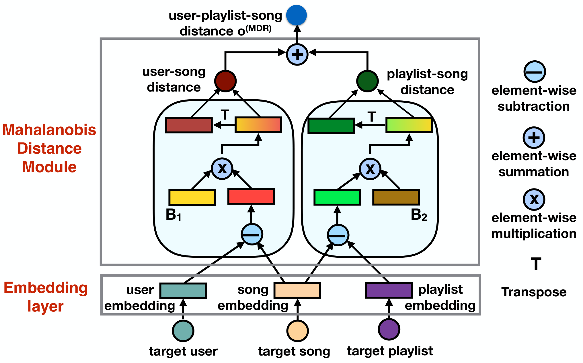
5.1.4. MDR Design
The MDR architecture is depicted in Figure 2. It has an Input, Embedding Layer, and Mahalanobis Distance Module.
Input: MDR takes a target user (user ID), a target playlist (playlist ID), and a target song (song ID) as input.
Embedding Layer: MDR maintains three embedding matrices of users, playlists, and songs. By passing user , playlist , and song through the embedding layer, we obtain their respective embedding vectors , , and , where is the embedding size.
Mahalanobis Distance Module: As depicted in Figure 2, this module outputs a distance score that indicates the relevance of candidate song to both user ’s music preference and playlist ’s theme. Intuitively, the lower the distance score is, the more relevant the song is. is computed as follows:
| (11) |
where is song ’s bias, and are quadratic Mahalanobis distance scores between user and song , and between playlist and song , shown in the following two equations. and are two metric learning vectors. And,
5.2. Mahalanobis distance-based Attentive Song Similarity recommender (MASS)
As stated in the Section 1, MASS belongs to Group 2, where it measures attentive similarities between the target song and member songs in the target playlist. An overview of MASS’s architecture is depicted in Figure 3. MASS has five components: Input, Embedding Layer, Processing Layer, Attention Layer, and Output.

5.2.1. Input:
The inputs to our MASS model include a target user , a candidate song for a target playlist , and a list of member songs within the playlist, where is the number of songs in the largest playlist (i.e., containing the largest number of songs) in the dataset. If a playlist contains less than songs, we pad the list with zeroes until it reaches length .
5.2.2. Embedding Layer:
This layer holds two embedding matrices: a user embedding matrix and a song embedding matrix . By passing the input target user and target song through these two respective matrices, we obtain their embedding vectors and . Similarly, we acquire the embedding vectors for all member songs in , denoted by .
5.2.3. Processing Layer:
We first need to consolidate and . Following widely adopted deep multimodal network designs (Srivastava and Salakhutdinov 2012), we concatenate the two embeddings, and then transform them into a new vector via a fully connected layer with weight matrix , bias term , and activation function ReLU. We formulate this process as follows:
| (12) |
Note that can be interpreted as a search query in QA systems (Xiong et al. 2016; Antol et al. 2015). Since we combined the target user with the query song (to add to the user’s target playlist), the search query is personalized. The ReLU activation function models a non-linear combination between these two target entities, and was chosen over sigmoid or tanh due to its encouragement of sparse activations and proven non-saturation (Glorot et al. 2011), which helps prevent overfitting.
Next, given the embedding vectors of the member songs in target playlist , we approximate the conditional probability P by:
| (13) |
where returns the Mahalanobis distance between two vectors, is the song bias reflecting its overall popularity, and is the attention score to weight the contribution of the partial distance between search query and member song . We will show how to calculate below, and in Attention Layer at 5.2.4.
As indicated in Eq. (3), we parameterize , which will be learned during the training phase. The Mahalanobis distance between the search query and each member song , treating as an edge-weight vector, is measured by:
| (14) |
|
Calculating Eq. (14) for every member song yields the following -dimensional vector:
| (15) |
Note that is shared across all Mahalanobis measurement pairs. Now we go into detail of how to calculate the attention weights using our proposed Attention Layer.
5.2.4. Attention Layer:
With distance scores obtained in Eq. (15), we need to combine them into one distance value to reflect how relevant the target song is w.r.t the target playlist’s member songs. The simplest approach is to follow the well-known item similarity design (Ning and Karypis 2011; Kabbur et al. 2013) where the same weights are assigned for all distance scores. This is sub-optimal in our domain because different member song can relate to the target song differently. For example, given a country playlist and a target song of the same genre, the member songs that share the same artist with the target song would be more similar to the target song than the other member songs in the playlist. To address this concern, we propose a novel memory metric-based attention mechanism to properly allocate different attentive scores to the distance values in Eq. (15). Compared to existing attention mechanisms, our attention mechanism maintains its own embedding memory of users and songs (i.e., memory-based property), which can function as an external memory. It also computes attentive scores using Mahalanobis distance (i.e., metric-based property) instead of traditional dot product. Note that the memory-based property is also commonly applied to question-answering in NLP, where memory networks have utilized external memory (Sukhbaatar et al. 2015) for better memorization of context information (Kumar et al. 2016; Miller et al. 2016). Our attention mechanism has one external memory containing user and song embedding matrices. When the user and song embedding matrices of our attention mechanism are identical to those in the embedding layer, it is the same as looking up the embedding vectors of target users, target songs, and member songs in the embedding layer (Section 5.2.2). Therefore, using external memory will make room for more flexibility in our models.
The attention layer features an external user embedding matrix and external song embedding matrix . Given the following inputs – a target user , a target song , and all member songs in playlist – by passing them through the corresponding embedding matrices, we obtain the embedding vectors of , , and all the member songs, denoted as , , and , respectively.
We then forge a personalized search query by combining and in a multimodal design as follows:
| (16) |
where is a weight matrix and is a bias term. Next, we measure the Mahalanobis distance (with an edge weight vector ) from to a member song’s embedding vector where :
| (17) |
|
Using Eq. (17), we generate distance scores between each of member songs and the candidate song. Then we apply softmin on distance scores in order to obtain the member songs’ attentive scores55 5 Note that attentive scores of padded items are 0.. Intuitively, the lower the distance between a search query and a member song vector, the higher its contribution level is w.r.t the candidate song.
| (18) |
5.2.5. Output:
5.3. Mahalanobis distance based Attentive Song Recommender (MASR = MDR + MASS)
We enhance our performance on the APC problem by combining our MDR and MASS into a Mahalanobis distance based Attentive Song Recommender (MASR) model. MASR outputs a cumulative distance score from the outputs of MDR and MASS as follows:
| (20) |
where is from Eq. (11), is from Eq. (19), and is a hyperparameter to adjust the contribution levels of MDR and MASS. can be tuned using a development dataset. However, in the following experiments, we set to receive equal contribution from MDR and MASS. We pretrain MDR and MASS first, then fix MDR and MASS’s parameters in MASR. There are two benefits of this design. First, if MASR is learnable with pretrained MDR and MASS initialization, MASR would have too high a computational cost to train. Second, by making MASR non-learnable, MDR and MASS in MASR can be trained separately and in parallel, which is more practical and efficient for real-world systems.
5.4. Parameter Estimation
5.4.1. Learning with Bayesian Personalized Ranking (BPR) loss
We apply BPR loss as an objective function to train our MDR, MASS, MASR as follows:
| (21) |
|
where is a quartet of a target user, a target playlist, a positive song, and a negative song which is randomly sampled. is the sigmoid function; denotes all training instances; are the model’s parameters (for instance, in the MASS model); is a regularization hyper-parameter; and is the output of either MDR, MASS, or MASR, which is measured in Eq. (11), (19), and (20), respectively.
5.4.2. Learning with Adversarial Personalized Ranking (APR) loss
It has been shown in (He et al. 2018) that BPR loss is vulnerable to adversarial noise, and APR was proposed to enhance the robustness of a simple matrix factorization model. In this work, we apply APR to further improve the robustness of our MDR, MASS, and MASR. We name our MDR, MASS, and MASR trained with APR loss as AMDR, AMASS, AMASR by adding an “adversarial (A)” term, respectively. Denote as adversarial noise on the model’s parameters . The BPR loss from adding adversarial noise to is defined by:
| (22) |
where is optimized in Eq. (21) and fixed as constants in Eq. (22). Then, training with APR aims to play a minimax game as follows:
| (23) |
where is a hyper-parameter to control the magnitude of perturbations . In (He et al. 2018), the authors fixed for all the model’s parameters, which is not ideal because different parameters can endure different levels of perturbation. If we add too large adversarial noise, the model’s performance will downgrade, while adding too small noise does not guarantee more robust models. Hence, we multiply with the standard deviation of the targeting parameter to provide a more flexible noise magnitude. For instance, the adversarial noise magnitude on parameter in AMASS model is . If the values in are widely dispersed, they are more vulnerable to attack, so the adversarial noise applied during training must be higher in order to improve robustness. Whereas if the values are centralized, they are already robust, so only a small noise magnitude is needed.
Learning with APR follows 4 steps: Step 1: unlike (He et al. 2018) where parameters are saved at the last training epoch, which can be over-fitted parameter values (e.g. some thousands of epoches for matrix factorization in (He et al. 2018)), we first learn our models’ parameters by minimizing Eq. (21) and save the best checkpoint based on evaluating on a development dataset. Step 2: with optimal learned in Step 1, in Eq. (22), we set and fix to learn . Step 3: with optimal learned in Eq. (22), in Eq. (23) we set and fix to learn new values for . Step 4: We repeat Step 2 and Step 3 until a maximum number of epochs is reached and save the best checkpoint based on evaluation on a development dataset. Following (He et al. 2018; Kurakin et al. 2016), the update rule for is obtained by using the fast gradient method as follows:
| (24) |
Note that update rules of parameters in can be easily obtained by computing the partial derivative w.r.t each parameter in .
5.5. Time Complexity
Let denote the total number of training instances (= where refers to the number of songs in training playlist ). , denotes the maximum number of songs in all playlists. For each forward pass, MDR takes to measure (in Eq. (11)) for a positive training instance, and another forward pass with to calculate for a negative instance. The backpropagation for updating parameters take the same complexity. Therefore, the time complexity of MDR is . Similarly, for each positive training instance, MASS takes (i) to make each query in Eq. (12) and Eq. (16); (ii) to calculate distance scores from member songs to the target song in Eq. (15); and (iii) to measure attention scores in Eq. (18). Since embedding size is often small, is a dominant term and MASS’s time complexity is . Hence, both MDR and MASS scale linearly to the number of training instances and can run very fast, especially with sparse datasets. When training with APR, updating in Eq. (24) with fixed needs one forward and one backward pass. Learning in Eq. (23) requires one forward pass to measure in Eq. (21), one forward pass to measure in Eq. (22), and one backward pass to update in Eq. (23). Hence, time complexity when training with APR is times higher ( is small) compared to training with BPR loss.
6. Empirical study
6.1. Datasets
To evaluate our proposed models and existing baselines, we used two publicly accessible real-world datasets that contain user, playlist, and song information. They are described as follows:
-
30Music (Turrin et al. 2015): This is a collection of playlists data retrieved from Internet radio stations through Last.fm66 6 https://www.last.fm. It consists of 57K playlists and 466K songs from 15K users.
-
AOTM (McFee and Lanckriet 2012a): This dataset was collected from the Art of the Mix77 7 http://www.artofthemix.org/ playlist database. It consists of 101K playlists and 504K songs from 16K users, spanning from Jan 1998 to June 2011.
| Statistics | 30Music | AOTM |
|---|---|---|
| # of users | 12,336 | 15,835 |
| # of playlists | 32,140 | 99,903 |
| # of songs | 276,142 | 504,283 |
| # of interactions | 666,788 | 1,966,795 |
| avg. # of playlists per user | 2.6 | 6.3 |
| avg. & max # of songs per playlist | 18.75 & 63 | 17.69 & 58 |
| Density | 0.008% | 0.004% |
For data preprocessing, we removed duplicate songs in playlists. Then we adopted a widely used k-core preprocessing step (Tran et al. 2018; He and McAuley 2016) (with k-core = 5), filtering out playlists with less than 5 songs. We also removed users with an extremely large number of playlists, and extremely large playlists (i.e., containing thousands of songs). Since the datasets did not have song order information for playlists (i.e., which song was added to a playlist first, then next, and so on), we randomly shuffled the song order of each playlist and used it in the sequential recommendation baseline models to compare with our models. The two datasets are implicit feedback datasets. The statistics of the preprocessed datasets are presented in Table 1.
6.2. Baselines
We compared our proposed models with eight strong state-of-the-art models in the APC task. The baselines were trained by using BPR loss for a fair comparison:
-
Bayesian Personalized Ranking (MF-BPR) (Rendle et al. 2009): It is a pairwise matrix factorization method for implicit feedback datasets.
-
Collaborative Metric Learning (CML) (Hsieh et al. 2017): It is a collaborative metric-based method. It adopted Euclidean distance to measure a user’s preference on items.
-
Neural Collaborative Filtering (NeuMF++) (He et al. 2017b): It is a neural network based method that models non-linear user-item interactions. We pretrained two components of NeuMF to obtain its best performance (i.e., NeuMF++).
-
Factored Item Similarity Methods (FISM) (Kabbur et al. 2013): It is a item neighborhood-based method. It ranks a candidate song based on its similarity with member songs using dot product.
-
Collaborative Memory Network (CMN++) (Ebesu et al. 2018): It is a user-neighborhood based model using a memory network to assign attentive scores for similar users.
-
Personalized Ranking Metric Embedding (PRME) (Feng et al. 2015): It is a sequential recommender that models a personalized first-order Markov behavior using Euclidean distance.
-
Translation-based Recommendation (Transrec) (He et al. 2017a): It is one of the best sequential recommendation methods. It models the third order between the user, the previous song, and the next song where the user acts as a translator.
-
Convolutional Sequence Embedding Recommendation
(Caser) (Tang and Wang 2018): It is a CNN based sequential recommendation. It embeds a sequence of recent songs into an “image” in time and latent spaces, then learns sequential patterns as local features of the image using different horizontal and vertical filters.
We did not compare our models with baselines that performed worse than above listed baselines like item-KNN(Sarwar et al. 2001), SLIM(Ning and Karypis 2011), etc.
MF-BPR, CML, and NeuMF++ used only user/playlist-song interaction data to model either users’ preferences over songs P() or playlists’ tastes over songs P(). We ran the baselines both ways, and report the best results. Two neighborhood-based baselines utilized neighbor users/playlists (i.e., CMN++) or member songs (i.e., FISM) to recommend the next song based on user/playlist similarities or song similarities (i.e., measure P() and P(), of which we report the best results).
| Methods | 30Music | AOTM | |||
| hit@10 | ndcg@10 | hit@10 | ndcg@10 | ||
| (a) | MF-BPR | 0.450 | 0.315 | 0.699 | 0.473 |
| (b) | CML | 0.600 | 0.452 | 0.735 | 0.481 |
| (c) | NeuMF++ | 0.623 | 0.461 | 0.741 | 0.498 |
| (d) | FISM | 0.544 | 0.346 | 0.686 | 0.446 |
| (e) | CMN++ | 0.536 | 0.397 | 0.722 | 0.505 |
| (f) | PRME | 0.426 | 0.260 | 0.570 | 0.354 |
| (g) | Transrec | 0.570 | 0.417 | 0.710 | 0.450 |
| (h) | Caser | 0.458 | 0.289 | 0.681 | 0.448 |
| Ours | MDR | 0.705 | 0.524 | 0.820 | 0.631 |
| MASS | 0.670 | 0.500 | 0.834 | 0.639 | |
| MASR | 0.731 | 0.564 | 0.854 | 0.654 | |
| AMDR | 0.764 | 0.581 | 0.850 | 0.658 | |
| AMASS | 0.753 | 0.581 | 0.856 | 0.659 | |
| AMASR | 0.785 | 0.604 | 0.874 | 0.677 | |
| Imprv. (%) | MASR | +17.34 | +22.34 | +13.36 | +28.24 |
| AMASR | +26.00 | +31.02 | +17.95 | +34.19 | |
6.3. Experimental Settings
Protocol: We use the widely adopted leave-one-out evaluation setting (He et al. 2017b). Since both the 30Music and AOTM datasets do not contain timestamps of added songs for each playlist, we randomly sample two songs per playlist–one for a positive test sample, and one for a development set to tune hyper-parameters–while the remaining songs in each playlist make up the training set. We follow (He et al. 2017b; Tran et al. 2019) and uniformly random sample 100 non-member songs as negative songs, and rank the test song against those negative songs.
Evaluation metrics: We evaluate the performance of the models with two widely used metrics: Hit Ratio (hit@N), and Normalized Discounted Cumulative Gain (NDCG@N). The hit@N measures whether the test item is in the recommended list or not, while the NDCG@N takes into account the position of the hit and assigns higher scores to hits at top-rank positions. For the test set, we measure both metrics and report the average scores.
Hyper-parameters settings: Models are trained with the Adam optimizer with learning rates from {0.001, 0.0001}, regularization terms from {0, 0.1, 0.01, 0.001, 0.0001}, and embedding sizes from {8, 16, 32, 64}. The maximum number of epochs is 50, and the batch size is 256. The number of hops in CMN++ are selected from {1, 2, 3, 4}. In NeuMF++, the number of MLP layers are selected from {1, 2, 3}. The number of negative samples per one positive instance is 4, similar to (He et al. 2017b). The Markov order in Caser is selected from {4, 5, 6, 7, 8, 9, 10}. For APR training, the number of APR training epochs is 50, the noise magnitude is selected from {0.5, 1.0}, and the adversarial regularization is set to 1, as suggested in (He et al. 2018). Adversarial noise is added only in training process, and are initialized as zero. All hyper-parameters are tuned by using the development set. Our source code is available at https://github.com/thanhdtran/MASR.git.
| Methods | 30Music | AOTM | RI(%) | ||
|---|---|---|---|---|---|
| hit@10 | ndcg@10 | hit@10 | ndcg@10 | ||
| MDR_us | 0.684 | 0.500 | 0.815 | 0.594 | +3.68 |
| MDR_ps | 0.654 | 0.476 | 0.746 | 0.547 | +10.79 |
| MDR_ups (i.e., MDR) | 0.705 | 0.524 | 0.818 | 0.613 | |
| MASS_ups | 0.651 | 0.479 | 0.789 | 0.581 | +4.12 |
| MASS_ps | 0.621 | 0.450 | 0.764 | 0.523 | +10.82 |
| MASS_us (i.e., MASS) | 0.670 | 0.500 | 0.820 | 0.631 | |
6.4. Experimental Results
6.4.1. Performance comparison
Table 2 shows the performance of our proposed models and baselines on each dataset. MDR and baselines (a)-(c) are in Group 1, but MDR shows much better performance compared to the (a)-(c) baselines, improving at least 11.14% hit@10 and 18.81% NDCG@10 on average. CML simply adopts Euclidean distance between users/playlists and positive songs, but has nearly equal performance with NeuMF++, which utilizes a neural network to learn non-linear relationships between users/playlists and songs. This result shows the effectiveness of using metric learning over dot product in recommendation. MDR outperforms CML by 19.04% on average. This confirms the effectiveness of Mahalanobis distance over Euclidian distance for recommendation.
MASS outperforms both FISM and CMN++, improving hit@10 by 18.4%, and NDCG@10 by 25.5% on average. This is because FISM does not consider the attentive contribution of different neighbors. Even though CMN++ can assign attention scores for different user/playlist neighbors, it bears the flaws of Group 1 by considering only either neighbor users or neighbor playlists. More importantly, MASS uses a novel attentive metric design, while dot product is utilized in FISM and CMN++. Sequential models, (f)-(h) baselines, do not work well. In particular, MASS outperforms the (f)-(h) baselines, improving 24.6% on average compared to the best model in (f)-(h).
MASR outperforms both MDR and MASS, indicating the effectiveness of fusing them into one model. Particularly, MASR improves MDR by 5.0%, and MASS by 6.7% on average. Performances of MDR, MASS, MASR are boosted when adopting APR loss with a flexible noise magnitude. AMDR improves MDR by 7.7%, AMASS improves MASS by 9.4%, and AMASR improves MASR by 5.8%. We also compare our flexible noise magnitude with a fixed noise magnitude used in (He et al. 2018) by varying the fixed noise magnitude in {0.5, 1.0} and setting . We observe that APR with a flexible noise magnitude performs better with an average improvement of 7.53%.
Next, we build variants of our MDR and MASS models by removing either playlist or user embeddings, or using both of them. Table 3 presents an ablation study of exploiting playlist embeddings. MDR_us is the MDR that uses only user-song interactions (i.e., ignore playlist-song distance in Eq. (11)). MDR_ps is the MDR that uses only playlist-song interactions (i.e., ignores user-song distance in Eq. (11)). MDR_ups is our proposed MDR model. Similarly, MASS_ups is the MASS model but considers both user-song distances and playlist-song distances in its design. The Embedding Layer and Attention Layer of MASS_ups have additional playlist embedding matrices and , respectively. MASS_ps is the MASS model that replaces user embeddings with playlist embeddings. MASS_us is our proposed MASS model.
MDR (i.e., MDR_ups) outperforms its derived forms (MDR_us and MDR_ps), improving by 3.710.8% on average. This result shows the effectiveness of modeling both users’ preferences and playlists’ themes in MDR design. MASS (i.e., MASS_us) outperforms its two variants (MASS_ups and MASS_ps), improving MASS_ups by 3.7%, and MASS_ps by 10.8% on average. It makes sense that using additional playlist embeddings in MASS_ups is redundant since the member songs have already conveyed the playlist’s theme, and ignoring user embeddings in MASS_ps neglects user preferences.
6.4.2. Varying top-N recommendation list and embedding size
Figure 4 shows performances of all models when varying top-N recommendation from 1 to 10. We see that all models gain higher results when increasing top-N, and all our proposed models outperform all baselines across all top-N values. On average, MASR improves 26.3%, and AMASR improves 33.9% over the best baseline’s performance.
Figure 588 8 Figure 5 shares the same legend with Figure 4 for saving space. shows all models’ performances when varying the embedding size from {8, 16, 32, 64} for the 30Music dataset. Note that the AOTM dataset also shows similar results but is omitted due to the space limitations. We observe that most models tend to have increased performance when increasing embedding size. AMDR does not improve MDR when but does so when increasing . This phenomenon was also reported in (He et al. 2018) because when , MDR is too simple and has a small number of parameters, which is far from overfitting the data and not very vulnerable to adversarial noise. However, for more complicated models like MASS and MASR, even with a small embedding size , APR shows its effectiveness in making the models more robust, and leads to an improvement of AMASS by 12.0% over MASS, and an improvement of AMASR by 7.5% over MASR. The improvements of AMDR, AMASS, AMASR over their corresponding base models are higher for larger due to the increase of model complexity.
| Attention Types | 30Music | AOTM | RI(%) | ||
|---|---|---|---|---|---|
| hit@10 | ndcg@10 | hit@10 | ndcg@10 | ||
| non-mem + dot | 0.630 | 0.454 | 0.785 | 0.574 | +8.51 |
| non-mem + metric | 0.660 | 0.490 | 0.803 | 0.601 | +3.43 |
| mem + dot | 0.659 | 0.475 | 0.791 | 0.585 | +5.40 |
| mem + metric | 0.670 | 0.500 | 0.834 | 0.639 | |


6.4.3. Is our memory metric-based attention helpful?
To answer this question, we evaluate how MASS’s performance changed when varying its attention mechanism as follows:
-
non-memory + dot product (non-mem + dot): It is the popular dot attention introduced in (Luong et al. 2015).
-
non-memory + metric (non-mem + metric): It is our proposed attention with Mahalanobis distance but no external memory.
-
memory + dot product (mem + dot): It is the dot attention but exploiting external memory.
-
memory + metric (mem + metric): It is our proposed attention mechanism.
We do not compare with the no-attention case because literature has already proved the effectiveness of the attention mechanism (Vaswani et al. 2017). Table 4 shows the performance of MASS under the variations of our proposed attention mechanism. We have some key observations. First, non-mem + metric attention outperforms non-mem + dot attention with an improvement of 4.9% on average. Similarly, mem + metric attention improves the mem + dot attention design by 5.4% on average. This enhancement comes from different nature of metric space and dot product space. Moreover, these results confirm that metric-based attention designs fit better into our proposed Mahalanobis distance based model. Second, memory based attention works better than non-mem attention. Particularly, on average, mem + dot improves non-mem + dot by 2.98%, and mem + metric improves non-mem + metric by 3.43%. Overall, the performance order is mem + metric > non-mem + metric > mem + dot > non-mem + dot, which confirms that our proposed attention performs the best and improves 3.438.51% compared to its variations.
6.4.4. Deep analysis on attention
To further understand how attention mechanisms work, we connect attentive scores generated by attention mechanisms with Pointwise Mutual Information scores. Given a target song and a member song , the PMI score between them is defined as: . Here, PMI(k,t) score indicates how likely two songs and co-occur together, or how likely a target song will be added into song ’s playlist.
Given a playlist that has a set of member songs, we measure PMI scores between the target song and each of member songs. Then, we apply to those PMI scores to obtain PMI attentive scores. Intuitively, the member song that has a higher PMI score with candidate song (i.e., co-occurs more with song ) will have a higher PMI attentive score. We draw scatter plots between PMI attentive scores and attentive scores generated by our proposed attention mechanism and its variations. Figure 6 shows the experimental results. We observe that the Pearson correlation between the PMI attentive scores and the attentive scores generated by our attention mechanism is the highest (0.254). This result shows that our proposed attention tends to give higher scores to co-occurred songs, which is what we desire. The Pearson correlation results are also consistent with what was reported in Table 4.
6.4.5. Runtime comparison
To compare model runtimes, we used a Nvidia GeForce GTX 1080 Ti with a batch size of 256 and embedding size of 64. We do not report MASR and AMASR’s runtimes because their components are pretrained and fixed (i.e., there is no learning process/time). Figure 7 shows the runtimes (seconds per epoch) of our models and the baselines for each dataset. MDR only took 39 and 173 seconds per epoch in 30Music and AOTM, respectively, while MASS took 88 and 375 seconds. MDR, one of the fastest models, was also competitive with CML and MF-BPR.
7. Conclusion
In this work, we proposed three novel recommendation approaches based on Mahalanobis distance. Our MDR model used Mahalanobis distance to account for both users’ preferences and playlists’ themes over songs. Our MASS model measured attentive similarities between a candidate song and member songs in a target playlist through our proposed memory metric-based attention mechanism. Our MASR model combined the capabilities of MDR and MASR. We also adopted and customized Adversarial Personalized Ranking (APR) loss with proposed flexible noise magnitude to further enhance the robustness of our three models. Through extensive experiments against eight baselines in two real-world large-scale APC datasets, we showed that our MASR improved 20.3%, and AMASR using APR loss improved 27.3% on average over the best baseline. Our runtime experiments also showed that our models were not only competitive, but fast as well.
Acknowledgment
This work was supported in part by NSF grant CNS-1755536, Google Faculty Research Award, Microsoft Azure Research Award, AWS Cloud Credits for Research, and Google Cloud. Any opinions, findings and conclusions or recommendations expressed in this material are the author(s) and do not necessarily reflect those of the sponsors.
References
- (1)
- Aizenberg et al. (2012) Natalie Aizenberg, Yehuda Koren, and Oren Somekh. 2012. Build your own music recommender by modeling internet radio streams. In WWW. 1–10.
- Antol et al. (2015) Stanislaw Antol, Aishwarya Agrawal, Jiasen Lu, Margaret Mitchell, Dhruv Batra, C Lawrence Zitnick, and Devi Parikh. 2015. Vqa: Visual question answering. In ICCV. 2425–2433.
- Bahdanau et al. (2014) Dzmitry Bahdanau, Kyunghyun Cho, and Yoshua Bengio. 2014. Neural machine translation by jointly learning to align and translate. arXiv preprint arXiv:1409.0473 (2014).
- Chen et al. (2012) Shuo Chen, Josh L Moore, Douglas Turnbull, and Thorsten Joachims. 2012. Playlist prediction via metric embedding. In SIGKDD. 714–722.
- Devooght et al. (2015) Robin Devooght, Nicolas Kourtellis, and Amin Mantrach. 2015. Dynamic matrix factorization with priors on unknown values. In SIGKDD. 189–198.
- Donkers et al. (2017) Tim Donkers, Benedikt Loepp, and Jürgen Ziegler. 2017. Sequential user-based recurrent neural network recommendations. In RecSys. 152–160.
- Ebesu et al. (2018) Travis Ebesu, Bin Shen, and Yi Fang. 2018. Collaborative Memory Network for Recommendation Systems. arXiv preprint arXiv:1804.10862 (2018).
- Feng et al. (2015) Shanshan Feng, Xutao Li, Yifeng Zeng, Gao Cong, Yeow Meng Chee, and Quan Yuan. 2015. Personalized Ranking Metric Embedding for Next New POI Recommendation.. In IJCAI. 2069–2075.
- Flexer et al. (2008) Arthur Flexer, Dominik Schnitzer, Martin Gasser, and Gerhard Widmer. 2008. Playlist Generation using Start and End Songs.. In ISMIR, Vol. 8. 173–178.
- Glorot et al. (2011) Xavier Glorot, Antoine Bordes, and Yoshua Bengio. 2011. Deep sparse rectifier neural networks. In AISTATS. 315–323.
- He et al. (2017a) Ruining He, Wang-Cheng Kang, and Julian McAuley. 2017a. Translation-based recommendation. In RecSys. 161–169.
- He and McAuley (2016) Ruining He and Julian McAuley. 2016. Ups and downs: Modeling the visual evolution of fashion trends with one-class collaborative filtering. In WWW. 507–517.
- He et al. (2018) Xiangnan He, Zhankui He, Xiaoyu Du, and Tat-Seng Chua. 2018. Adversarial personalized ranking for recommendation. In SIGIR. 355–364.
- He et al. (2017b) Xiangnan He, Lizi Liao, Hanwang Zhang, Liqiang Nie, Xia Hu, and Tat-Seng Chua. 2017b. Neural collaborative filtering. In WWW. 173–182.
- He et al. (2016) Xiangnan He, Hanwang Zhang, Min-Yen Kan, and Tat-Seng Chua. 2016. Fast matrix factorization for online recommendation with implicit feedback. In SIGIR. 549–558.
- Hidasi and Karatzoglou (2018) Balázs Hidasi and Alexandros Karatzoglou. 2018. Recurrent neural networks with top-k gains for session-based recommendations. In CIKM. 843–852.
- Hsieh et al. (2017) Cheng-Kang Hsieh, Longqi Yang, Yin Cui, Tsung-Yi Lin, Serge Belongie, and Deborah Estrin. 2017. Collaborative metric learning. In WWW. 193–201.
- Hu et al. (2008) Yifan Hu, Yehuda Koren, and Chris Volinsky. 2008. Collaborative filtering for implicit feedback datasets. In ICDM. 263–272.
- Jannach et al. (2017) Dietmar Jannach, Iman Kamehkhosh, and Lukas Lerche. 2017. Leveraging multi-dimensional user models for personalized next-track music recommendation. In SIGAPP. 1635–1642.
- Jing and Smola (2017) How Jing and Alexander J Smola. 2017. Neural survival recommender. In WSDM. 515–524.
- Kabbur et al. (2013) Santosh Kabbur, Xia Ning, and George Karypis. 2013. Fism: factored item similarity models for top-n recommender systems. In SIGKDD. 659–667.
- Kamehkhosh and Jannach (2017) Iman Kamehkhosh and Dietmar Jannach. 2017. User perception of next-track music recommendations. In UMAP. 113–121.
- Koren (2009) Yehuda Koren. 2009. Collaborative filtering with temporal dynamics. In SIGKDD. 447–456.
- Koren et al. (2009) Yehuda Koren, Robert Bell, and Chris Volinsky. 2009. Matrix factorization techniques for recommender systems. Computer 8 (2009), 30–37.
- Kumar et al. (2016) Ankit Kumar, Ozan Irsoy, Peter Ondruska, Mohit Iyyer, James Bradbury, Ishaan Gulrajani, Victor Zhong, Romain Paulus, and Richard Socher. 2016. Ask me anything: Dynamic memory networks for natural language processing. In ICML. 1378–1387.
- Kurakin et al. (2016) Alexey Kurakin, Ian Goodfellow, and Samy Bengio. 2016. Adversarial examples in the physical world. arXiv preprint arXiv:1607.02533 (2016).
- Liang et al. (2018) Dawen Liang, Rahul G Krishnan, Matthew D Hoffman, and Tony Jebara. 2018. Variational Autoencoders for Collaborative Filtering. arXiv preprint arXiv:1802.05814 (2018).
- Liang et al. (2015) Dawen Liang, Minshu Zhan, and Daniel PW Ellis. 2015. Content-Aware Collaborative Music Recommendation Using Pre-trained Neural Networks.. In ISMIR. 295–301.
- Luong et al. (2015) Minh-Thang Luong, Hieu Pham, and Christopher D Manning. 2015. Effective approaches to attention-based neural machine translation. arXiv preprint arXiv:1508.04025 (2015).
- Ma et al. (2018a) Chen Ma, Peng Kang, Bin Wu, Qinglong Wang, and Xue Liu. 2018a. Gated Attentive-Autoencoder for Content-Aware Recommendation. arXiv preprint arXiv:1812.02869 (2018).
- Ma et al. (2018b) Chen Ma, Yingxue Zhang, Qinglong Wang, and Xue Liu. 2018b. Point-of-Interest Recommendation: Exploiting Self-Attentive Autoencoders with Neighbor-Aware Influence. In CIKM. 697–706.
- McFee and Lanckriet (2012a) B. McFee and G. R. G. Lanckriet. 2012a. Hypergraph models of playlist dialects. In ISMIR.
- McFee and Lanckriet (2012b) Brian McFee and Gert RG Lanckriet. 2012b. Hypergraph Models of Playlist Dialects.. In ISMIR, Vol. 12. 343–348.
- Miller et al. (2016) Alexander Miller, Adam Fisch, Jesse Dodge, Amir-Hossein Karimi, Antoine Bordes, and Jason Weston. 2016. Key-value memory networks for directly reading documents. arXiv preprint arXiv:1606.03126 (2016).
- Ning and Karypis (2011) Xia Ning and George Karypis. 2011. Slim: Sparse linear methods for top-n recommender systems. In ICDM. 497–506.
- Oramas et al. (2017) Sergio Oramas, Oriol Nieto, Mohamed Sordo, and Xavier Serra. 2017. A deep multimodal approach for cold-start music recommendation. arXiv preprint arXiv:1706.09739 (2017).
- Pichl et al. (2017) Martin Pichl, Eva Zangerle, and Günther Specht. 2017. Improving context-aware music recommender systems: beyond the pre-filtering approach. In ICMR. 201–208.
- Pohle et al. (2005) Tim Pohle, Elias Pampalk, and Gerhard Widmer. 2005. Generating similarity-based playlists using traveling salesman algorithms. In DAFx. 220–225.
- Ram and Gray (2012) Parikshit Ram and Alexander G Gray. 2012. Maximum inner-product search using cone trees. In SIGKDD. 931–939.
- Rendle et al. (2009) Steffen Rendle, Christoph Freudenthaler, Zeno Gantner, and Lars Schmidt-Thieme. 2009. BPR: Bayesian personalized ranking from implicit feedback. In UAI. 452–461.
- Rendle et al. (2010) Steffen Rendle, Christoph Freudenthaler, and Lars Schmidt-Thieme. 2010. Factorizing personalized markov chains for next-basket recommendation. In WWW. 811–820.
- Sarwar et al. (2001) Badrul Sarwar, George Karypis, Joseph Konstan, and John Riedl. 2001. Item-based collaborative filtering recommendation algorithms. In WWW. 285–295.
- Srivastava and Salakhutdinov (2012) Nitish Srivastava and Ruslan R Salakhutdinov. 2012. Multimodal learning with deep boltzmann machines. In NIPS. 2222–2230.
- Sukhbaatar et al. (2015) Sainbayar Sukhbaatar, Jason Weston, Rob Fergus, et al. 2015. End-to-end memory networks. In NIPS. 2440–2448.
- Tang and Wang (2018) Jiaxi Tang and Ke Wang. 2018. Personalized top-n sequential recommendation via convolutional sequence embedding. In WSDM. 565–573.
- Teinemaa et al. (2018) Irene Teinemaa, Niek Tax, and Carlos Bentes. 2018. Automatic Playlist Continuation through a Composition of Collaborative Filters. arXiv preprint arXiv:1808.04288 (2018).
- Tran et al. (2018) Thanh Tran, Kyumin Lee, Yiming Liao, and Dongwon Lee. 2018. Regularizing Matrix Factorization with User and Item Embeddings for Recommendation. In CIKM. 687–696.
- Tran et al. (2019) Thanh Tran, Xinyue Liu, Kyumin Lee, and Xiangnan Kong. 2019. Signed Distance-based Deep Memory Recommender. In WWW. 1841–1852.
- Turrin et al. (2015) Roberto Turrin, Massimo Quadrana, Andrea Condorelli, Roberto Pagano, and Paolo Cremonesi. 2015. 30Music Listening and Playlists Dataset.
- Vall et al. (2018) Andreu Vall, Matthias Dorfer, Markus Schedl, and Gerhard Widmer. 2018. A Hybrid Approach to Music Playlist Continuation Based on Playlist-Song Membership. arXiv preprint arXiv:1805.09557 (2018).
- Vall et al. (2017) Andreu Vall, Hamid Eghbal-Zadeh, Matthias Dorfer, Markus Schedl, and Gerhard Widmer. 2017. Music playlist continuation by learning from hand-curated examples and song features: Alleviating the cold-start problem for rare and out-of-set songs. In DLRS. 46–54.
- Van den Oord et al. (2013) Aaron Van den Oord, Sander Dieleman, and Benjamin Schrauwen. 2013. Deep content-based music recommendation. In NIPS. 2643–2651.
- Vaswani et al. (2017) Ashish Vaswani, Noam Shazeer, Niki Parmar, Jakob Uszkoreit, Llion Jones, Aidan N Gomez, Łukasz Kaiser, and Illia Polosukhin. 2017. Attention is all you need. In NIPS. 5998–6008.
- Wang et al. (2015) Pengfei Wang, Jiafeng Guo, Yanyan Lan, Jun Xu, Shengxian Wan, and Xueqi Cheng. 2015. Learning hierarchical representation model for nextbasket recommendation. In SIGIR. 403–412.
- Wang and Wang (2014) Xinxi Wang and Ye Wang. 2014. Improving content-based and hybrid music recommendation using deep learning. In SIGMM. 627–636.
- Wang et al. (2014) Xinxi Wang, Yi Wang, David Hsu, and Ye Wang. 2014. Exploration in interactive personalized music recommendation: a reinforcement learning approach. TOMM 11, 1 (2014), 7.
- Weinberger et al. (2006) Kilian Q Weinberger, John Blitzer, and Lawrence K Saul. 2006. Distance metric learning for large margin nearest neighbor classification. In NIPS. 1473–1480.
- Wu et al. (2016) Yao Wu, Christopher DuBois, Alice X Zheng, and Martin Ester. 2016. Collaborative denoising auto-encoders for top-n recommender systems. In WSDM. 153–162.
- Xing et al. (2003) Eric P Xing, Michael I Jordan, Stuart J Russell, and Andrew Y Ng. 2003. Distance metric learning with application to clustering with side-information. In NIPS. 521–528.
- Xiong et al. (2016) Caiming Xiong, Stephen Merity, and Richard Socher. 2016. Dynamic memory networks for visual and textual question answering. In ICML. 2397–2406.
- Yang et al. (2016) Zichao Yang, Diyi Yang, Chris Dyer, Xiaodong He, Alex Smola, and Eduard Hovy. 2016. Hierarchical attention networks for document classification. In NAACL HLT. 1480–1489.
- Zhu et al. (2019) Ziwei Zhu, Jianling Wang, and James Caverlee. 2019. Improving Top-K Recommendation via Joint Collaborative Autoencoders. In WWW.