跳到论文正文
W Papers独立论文阅读器 arXiv:1906.03403 论文正文 计算阅读时间 · 0%
引用这篇论文根据当前论文元数据生成,正式投稿前建议核对。


License: arXiv.org perpetual non-exclusive license
arXiv:1906.03403v3 [math.MG] 31 Aug 2020

Smocked Metric Spaces and their Tangent ConesThanks: We are grateful to SCGP and CUNYGC for hosting our meetings. Prof. Sormani’s research was funded in part by NSF DMS 1612049. Dr. Kazaras’ research was funded by SB and SCGP. The students were unfunded volunteers completing the work for research credit only.

Prof. Christina Sormani (Lehman and CUNYGC),
Dr. Demetre Kazaras (Stony Brook),
and Students:
David Afrifa (Lehman)
Victoria Antonetti (Lehman)
Moshe Dinowitz (Stony Brook)
Hindy Drillick (Stony Brook)
Maziar Farahzad (Stony Brook)
Shanell George (Lehman)
Aleah Lydeatte Hepburn (Lehman)
Leslie Trang Huynh (Lehman)
Emilio Minichiello (Queens)
Julinda Mujo Pillati (Lehman)
Srivishnupreeth Rendla (Stony Brook)
Ajmain Yamin (Stony Brook)
Address: Department of Mathematics
Lehman College
Bronx, NY 10468
Email address: sormanic@gmail.com Address: Department of Mathematics
CUNY Graduate Center
365 Fifth Avenue
NY NY 10016
Address: Department of Mathematics
Stony Brook University
100 Nicolls Rd,
Stony Brook, NY 11794
Email address: demetre.kazaras@stonybrook.edu
Abstract.

We introduce the notion of a smocked metric space and explore the balls and geodesics in a collection of different smocked spaces. We find their rescaled Gromov-Hausdorff limits and prove these tangent cones at infinity exist, are unique, and are normed spaces. We close with a variety of open questions suitable for advanced undergraduates, masters students, and doctoral students.

Key words and phrases: 
Smocked Metric Space, Gromov-Hausdorff, Tangent Space
2000 Mathematics Subject Classification
53C23, 54E35

1. Introduction

The asymptotic behavior of a metric space at infinity has been well studied by many mathematicians by taking a sequence of rescalings of the metric spaces and finding their Gromov-Hausdorff limit. This limit is called the tangent cone at infinity. This idea has ancient roots. For example, a hyperboloid rescaled in upon itself converges to a cone, which is equivalent to saying it is asymptotic to a cone at infinity. However for more abstract metric spaces, it can be more difficult to understand what it means to take a limit and it can be more difficult to find that limit. Often the limit is not unique and there is no reason for it to be a cone.

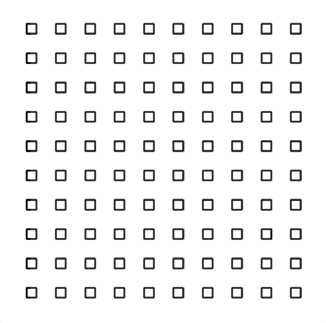
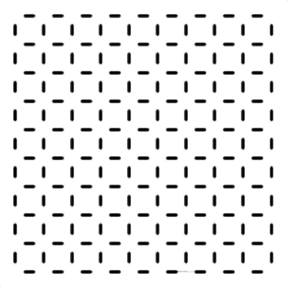
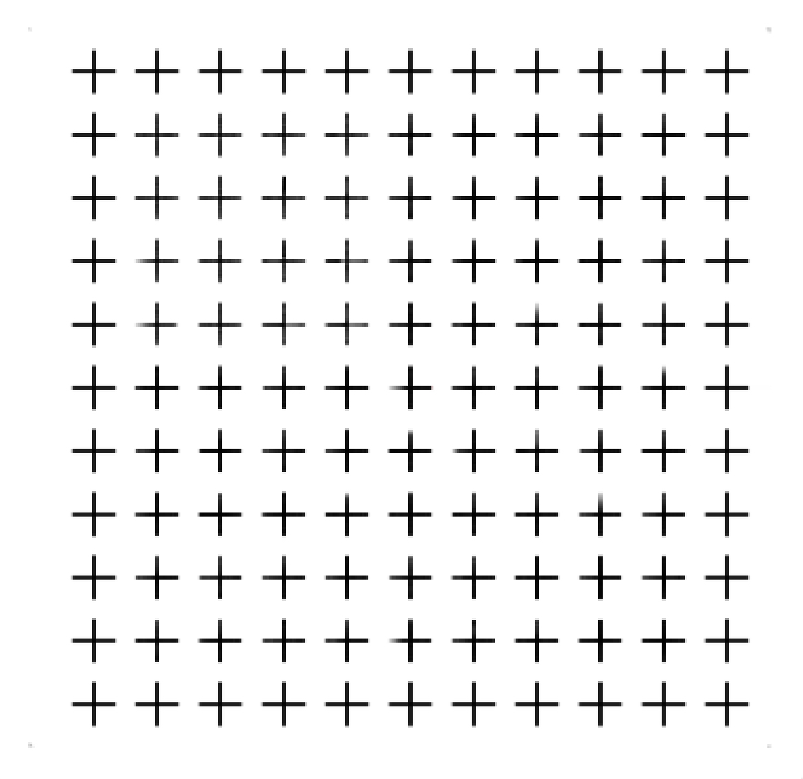
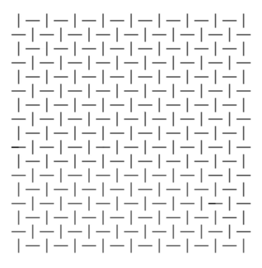
Here we introduce a new class of metric spaces that we call smocked spaces inspired by the craft of smocking fabric. Each smocked space is defined by taking a Euclidean space with a pattern on it (as in Figure 1) and then pulling each stitch in the pattern to a single point. The notion of pulling a thread to a point has already been explored by metric geometers as it provides interesting counter examples to questions involving areas and perimeters (cf. [2] by Burago-Ivanov). However this is the first time anyone has explored more complex patterns in which many threads are drawn to points. We discover that indeed we obtain some rather surprising tangent cones at infinity when studying these spaces.
Refer to caption
Refer to caption
Refer to caption
Refer to caption
Refer to caption
Refer to caption
Figure 1. The smocked spaces: X+X_{+}, XTX_{T}, X□X_{\square}, and XHX_{H}, X⋄X_{\diamond}, X=X_{=}.

We present the rigorous definition of a smocked space appears in Definition 3.1 after reviewing the definition of pulling a thread to a point in Definition 2.9. We prove some lemmas about balls in these spaces, which allow us to explore the balls of all six spaces on an intuitive level. We then choose three smocked spaces to analyze more deeply, ultimately determining their tangent cones at infinity in Theorem 9.2, Theorem 9.7, and Theorem 9.11. We’ve also proven a general theorem one can apply to find the Gromov-Hausdorff limit of a large class of smocking spaces in Theorem 9.1, while proving these tangent cones are unique and are normed spaces. In upcoming work by some of the authors [8], we complete the analysis of the other three smocked spaces and examine three dimensional versions of them as well. In upcoming work by Kazaras and Sormani [6], we will apply the results in these two papers to a question of Gromov and Sormani [4].11 1 Prof. Sormani’s grant NSF DMS 1612049 funds this overarching project on scalar curvature but the students were unpaid volunteers meeting in January 2019 at the CUNYGC and SCGP.

This paper can be read by anyone who has studied basic metric geometry as we review every concept before we need to apply it. Through the reading of this paper, one can learn the definition of Gromov-Hausdorff convergence, a standard technique for proving this convergence using correspondences, and the definition of the tangent cone at infinity of a metric space. As each concept is introduced, it is immediately applied to each of these patterns by various teams of students. It may be fun for the reader to find a smocking pattern online or in a smocking guide like [7] and work with it while reading this paper to discover something new. The reader might also slightly adapt the patterns explored within to see the consequences of altering the sizes of stitches and the spacing between them.

The paper closes with a section of open problems some of which are labeled as possible projects for an undergraduate or masters thesis. Other open problems are significantly more advanced. Students who would like to study metric geometry on a more advanced level are encouraged to read Burago-Burago-Ivanov’s award winning textbook [1].

2. Background

Here we quickly review metric spaces and pulled thread spaces. See also the award winning textbook by Burago-Burago-Ivanov [1]. If you already know these topics, just briefly glance through for notation.

2.1. Metric spaces by Prof. Sormani and Ajmain

Definition 2.1.

A metric space (X,d)(X,d) is a set XX with a function d:X×X→ℝd:X\times X\to\mathbb{R} satisfying the following:

  • •

    Nonnegativity: d⁡(x,y)≥0∀x,y∈X.\quad d(x,y)\geq 0\quad\forall x,y\in X.\quad

  • •

    Definiteness: d⁡(x,y)=0⇔x=y\quad d(x,y)=0\iff x=y.

  • •

    Symmetry: d⁡(x,y)=d⁡(y,x)∀x,y∈X.\quad d(x,y)=d(y,x)\quad\forall x,y\in X.

  • •

    The Triangle Inequality: d⁡(x,y)≤d⁡(x,z)+d⁡(z,y)∀x,y,z∈X.\quad d(x,y)\leq d(x,z)+d(z,y)\quad\forall x,y,z\in X.

In this paper we will use the following notation:

Definition 2.2.

Given a point pp in a metric space XX and r>0r>0. An open ball of radius rr about pp:

Br​(p)={x:d⁡(x,p)<r}.B_{r}(p)=\{x:\,d(x,p)<r\}. (2.1)

A closed ball of radius rr about pp:

B¯r​(p)={x:d⁡(x,p)≤r}.\bar{B}_{r}(p)=\{x:\,d(x,p)\leq r\}. (2.2)

A sphere of radius rr about pp:

∂Br​(p)={x:d⁡(x,p)=r}.\partial B_{r}(p)=\{x:\,d(x,p)=r\}. (2.3)
Definition 2.3.

Given a set KK in a metric space XX and r>0r>0, The tubular neighborhood of radius rr about KK:

Tr(K)={x:∃y∈Ks.t.d(x,y)<r}.T_{r}(K)=\{x:\,\exists y\in K\,s.t.\,d(x,y)<r\}. (2.4)
Lemma 2.4.

Given a point pp in a metric space XX and r,s>0r,s>0 we have

Ts​(Br​(p))=Br+s​(p).T_{s}(B_{r}(p))=B_{r+s}(p). (2.5)
Proof.

Let q∈Ts​(Br​(p))q\in T_{s}(B_{r}(p)). By the definition of tubular neighborhood, ∃y∈Br​(p)\exists y\in B_{r}(p) such that d⁡(q,y)<sd(q,y)<s. By the triangle inequality d⁡(q,p)<r+sd(q,p)<r+s, and therefore q∈Br+s​(p)q\in B_{r+s}(p) Now take q∈Br+s​(p)q\in B_{r+s}(p). So d⁡(q,p)<r+sd(q,p)<r+s. If Bs​(q)∩Br​(p)=∅B_{s}(q)\cap B_{r}(p)=\varnothing then r+s≤d⁡(q,p)r+s\leq d(q,p) which leads to a contradiction. Hence ∃y∈Br​(p)\exists y\in B_{r}(p) such that d⁡(y,q)<sd(y,q)<s, and so q∈Ts​(Br​(p))q\in T_{s}(B_{r}(p)). ∎

Lemma 2.5.

If K1⊂K2K_{1}\subset K_{2} then Ts​(K1)⊂Ts​(K2)T_{s}(K_{1})\subset T_{s}(K_{2}).

Proof.

Let p∈Ts​(K1)p\in T_{s}(K_{1}). Then ∃y∈K1\exists y\in K_{1} such that d⁡(p,y)<sd(p,y)<s. Since K1⊂K2K_{1}\subset K_{2}, we have ∃y∈K2\exists y\in K_{2} such that d⁡(p,y)∈sd(p,y)\in s. Thus p∈Ts​(K2)p\in T_{s}(K_{2}). ∎

Lemma 2.6.

Ts​(K1∪K2)=Ts​(K1)∪Ts​(K2)T_{s}(K_{1}\cup K_{2})=T_{s}(K_{1})\cup T_{s}(K_{2}).

Proof.

This follows from the definition of union:

Ts​(K1∪K2)\displaystyle T_{s}(K_{1}\cup K_{2}) =\displaystyle= {z:∃w∈K1∪K2s.t.d(z,w)<s}\displaystyle\{z:\,\exists w\in K_{1}\cup K_{2}\,s.t.\,d(z,w)<s\}
=\displaystyle= {z:∃w∈K1s.t.d(z,w)<sOR∃w∈K2s.t.d(z,w)<s}\displaystyle\{z:\,\exists w\in K_{1}\,s.t.\,d(z,w)<s\,OR\,\exists w\in K_{2}\,s.t.\,d(z,w)<s\}
=\displaystyle= {z:∃w∈K1s.t.d(z,w)<s}∪{z:∃w∈K2s.t.d(z,w)<s}\displaystyle\{z:\,\exists w\in K_{1}\,s.t.\,d(z,w)<s\}\cup\{z:\,\exists w\in K_{2}\,s.t.\,d(z,w)<s\}
=\displaystyle= Ts​(K1)∪Ts​(K2).\displaystyle T_{s}(K_{1})\cup T_{s}(K_{2}).

∎

Lemma 2.7.

Ts​(K1∩K2)⊂Ts​(K1)∩Ts​(K2)T_{s}(K_{1}\cap K_{2})\subset T_{s}(K_{1})\cap T_{s}(K_{2}).

Proof.

This follows from the definition of intersection:

Ts​(K1∪K2)\displaystyle T_{s}(K_{1}\cup K_{2}) =\displaystyle= {z:∃w∈K1∩K2s.t.d(z,w)<s}\displaystyle\{z:\,\exists w\in K_{1}\cap K_{2}\,s.t.\,d(z,w)<s\}
=\displaystyle= {z:∃w∈K1ANDK2s.t.d(z,w)<s}\displaystyle\{z:\,\exists w\in K_{1}\,AND\,K_{2}\,s.t.\,d(z,w)<s\}
⊂\displaystyle\subset {z:∃w∈K1s.t.d(z,w)<s}∩{z:∃w∈K2s.t.d(z,w)<s}\displaystyle\{z:\,\exists w\in K_{1}\,s.t.\,d(z,w)<s\}\cap\{z:\,\exists w\in K_{2}\,s.t.\,d(z,w)<s\}
=\displaystyle= Ts​(K1)∩Ts​(K2).\displaystyle T_{s}(K_{1})\cap T_{s}(K_{2}).

∎

Lemma 2.8.

In 𝔼2{\mathbb{E}}^{2} we have the following

Ts​([a,b]×{y})⊂[a−s,b+s]×[y−s,y+s]T_{s}([a,b]\times\{y\})\subset[a-s,b+s]\times[y-s,y+s] (2.6)
Ts​({x}×[a,b])⊂[x−s,x+s]×[a−s,b+s].T_{s}(\{x\}\times[a,b])\subset[x-s,x+s]\times[a-s,b+s]. (2.7)
Proof.

Let (p1,p2)∈Ts​([a,b]×{y})(p_{1},p_{2})\in T_{s}([a,b]\times\{y\}). Then ∃(q1,q2)∈[a,b]×{y}\exists(q_{1},q_{2})\in[a,b]\times\{y\} such that

d⁡(p,q)=(p1−q1)2+(p2−q2)2<s.d(p,q)=\sqrt{(p_{1}-q_{1})^{2}+(p_{2}-q_{2})^{2}}<s. (2.8)

Hence |p1−q1|<s|p_{1}-q_{1}|<s and |p2−q2|<s|p_{2}-q_{2}|<s. Therefore p∈[a−s,b+s]×[y−s,s+s]p\in[a-s,b+s]\times[y-s,s+s], as required. A similar argument shows Ts​({x}×[a,b])⊂[x−s,x+s]×[a−s,b+s]T_{s}(\{x\}\times[a,b])\subset[x-s,x+s]\times[a-s,b+s]. ∎

2.2. Pulled Thread Spaces by Prof. Sormani and Ajmain

Before introducing a smocked metric space we recall the notion of a pulled thread metric space, particularly in the setting where one starts with a Euclidean space, 𝔼N\mathbb{E}^{N}. The idea is that if one views a Euclidean plane as a cloth, and marks an interval on that cloth, then sews along that interval, and then pulls the thread tight, one obtains a new metric space (called a pulled strong space) in which the interval is now a point as in Figure 2.

Refer to caption
Figure 2. The distance between two points in a pulled thread space is the minimum of the length of the direct path and the sum of the lengths of a pair of segments touching the interval.
Definition 2.9.

Given a Euclidean space, 𝔼N\mathbb{E}^{N}, and an interval, II, one can define the pulled thread metric space, (X,d)(X,d), in which the interval is viewed as a single point.

X={x:x∈𝔼N∖I}∪{I}.X=\{x:\,x\in{\mathbb{E}^{N}}\setminus I\}\cup\{I\}. (2.9)

We have a pulled thread map π:𝔼N→X\pi:\mathbb{E}^{N}\to X such that π⁡(x)=x\pi(x)=x for x∈𝔼N∖Ix\in{\mathbb{E}^{N}}\setminus I and π⁡(x)=I\pi(x)=I for x∈Ix\in I. The distance function, d:X×X→[0,∞)d:X\times X\to[0,\infty), is defined by

d⁡(x,y)\displaystyle d(x,y) =\displaystyle= min{|x−y|,min{|x−z|+|z′−y|:z,z′∈I} for x,y∈𝔼N\displaystyle\min\{|x-y|,\min\{|x-z|+|z^{\prime}-y|:\,z,z^{\prime}\in I\}\quad\textrm{ for }x,y\in\mathbb{E}^{N} (2.10)
d⁡(x,I)\displaystyle d(x,I) =\displaystyle= min⁡{|x−z|:z∈I} for ​x∈𝔼N.\displaystyle\min\{|x-z|:\,z\in I\}\quad\textrm{ for }x\in\mathbb{E}^{N}. (2.11)

We can then define the pulled thread pseudometric d¯:𝔼N×𝔼N→[0,∞)\bar{d}:{\mathbb{E}^{N}}\times{\mathbb{E}^{N}}\to[0,\infty) to be

d¯(x,y)=d(π(x),π(y))=min{|x−y|,min{|x−z|+|z′−y|:z,z′∈I}.\bar{d}(x,y)=d(\pi(x),\pi(y))=\min\{|x-y|,\min\{|x-z|+|z^{\prime}-y|:\,z,z^{\prime}\in I\}. (2.12)

Finally we define the distance to the interval, D:𝔼N→[0,∞)D:{\mathbb{E}^{N}}\to[0,\infty):

D⁡(x)=min⁡{|x−z|:z∈I}=d⁡(π⁡(x),I).D(x)=\min\{|x-z|:\,z\in I\}=d(\pi(x),I). (2.13)

Notation: For any p∈Xp\in X, p≠Ip\neq I, write zpz_{p} to denote the unique point in II such that |p−zp|=d⁡(p,I)|p-z_{p}|=d(p,I).

Lemma 2.10.

A pulled thread space is a metric space.

Proof.

This has three parts:

Positive definiteness: d⁡(p,q)≥0d(p,q)\geq 0 and d⁡(p,q)=0⇔p=qd(p,q)=0\iff p=q:

The fact that d⁡(p,q)≥0d(p,q)\geq 0 for all p,q∈Xp,q\in X is clear from Definition 2.9. Suppose d⁡(p,q)=0d(p,q)=0 then p=π⁡(v)p=\pi(v) and q=π⁡(w)q=\pi(w) whereThen either

|v−w|=0⟹v=w⟹p=q|v-w|=0\implies v=w\implies p=q (2.14)

or there exists z,z′∈Iz,z^{\prime}\in I such that

|v−z|+|z′−w|=0|v-z|+|z^{\prime}-w|=0 (2.15)

which implies v=zv=z and z′=wz^{\prime}=w so v,w∈Iv,w\in I so

p=π⁡(v)=π⁡(w)=q.p=\pi(v)=\pi(w)=q. (2.16)

Symmetry d⁡(p,q)=d⁡(q,p)d(p,q)=d(q,p):

This follows by taking p=π⁡(x)p=\pi(x) and q=π⁡(y)q=\pi(y) and noting that

d⁡(p,q)\displaystyle d(p,q) =\displaystyle= min{|x−y|,min{|x−z|+|z′−y|:z,z′∈I}\displaystyle\min\{|x-y|,\min\{|x-z|+|z^{\prime}-y|:\,z,z^{\prime}\in I\} (2.17)
=\displaystyle= min{|y−x|,min{|y−z|+|z′−x|:z,z′∈I}=d(q,p).\displaystyle\min\{|y-x|,\min\{|y-z|+|z^{\prime}-x|:\,z,z^{\prime}\in I\}=d(q,p). (2.18)

Triangle inequality d⁡(a,b)≤d⁡(a,q)+d⁡(q,b)d(a,b)\leq d(a,q)+d(q,b):

We prove the triangle inequality in cases using the notation that for any p∈Xp\in X there exists vp∈𝔼Nv_{p}\in{\mathbb{E}}^{N} such that p=π⁡(vp)p=\pi(v_{p}) and if p≠Ip\neq I then there exists zp∈Iz_{p}\in I such that

d⁡(p,I)=|vp−zp|.d(p,I)=|v_{p}-z_{p}|. (2.19)

Case I: We assume a∈π⁡(X∖{I})a\in\pi(X\setminus\{I\}) and b=Ib=I (which also includes aa and bb switched by symmetry). This breaks into two cases:

Case I.a: We assume q=Iq=I, This implies d⁡(b,q)=0d(b,q)=0 and d⁡(a,q)=d⁡(b,q)d(a,q)=d(b,q) so

d⁡(a,b)=d⁡(a,q)+d⁡(q,b)d(a,b)=d(a,q)+d(q,b) (2.20)

Case I.b: We assume q≠Iq\neq I. This breaks into two deeper cases

Case I.b.i: We assume d⁡(a,q)=|a−q|d(a,q)=|a-q| which implies

d⁡(a,b)=|va−za|<|va−zq|≤|va−vq|−|vq−zq|=d⁡(a,q)+d⁡(q,b)\displaystyle d(a,b)=|v_{a}-z_{a}|<|v_{a}-z_{q}|\leq|v_{a}-v_{q}|-|v_{q}-z_{q}|=d(a,q)+d(q,b) (2.21)

Case I.b.ii: We assume d⁡(a,q)=|va−za|+|vq−zq|d(a,q)=|v_{a}-z_{a}|+|v_{q}-z_{q}| which implies

d⁡(a,b)=|va−za|<|va−zq​|+2|​vq−zq|=d⁡(a,q)+d⁡(q,b)\displaystyle d(a,b)=|v_{a}-z_{a}|<|v_{a}-z_{q}|+2|v_{q}-z_{q}|=d(a,q)+d(q,b) (2.22)

Case II : We assume a,b∈π⁡(X∖{I})a,b\in\pi(X\setminus\{I\}). This breaks into two cases:

Case II.a: We assume q=Iq=I which implies

d⁡(a,b)≤|va−za|+|vb−zb|=d⁡(a,q)+d⁡(q,b)d(a,b)\leq|v_{a}-z_{a}|+|v_{b}-z_{b}|=d(a,q)+d(q,b) (2.23)

Case II.b: We assume q≠Iq\neq I. This breaks into four deeper cases:

Case II.b.i: We assume d⁡(a,q)=|va−za|+|vq−zq|d(a,q)=|v_{a}-z_{a}|+|v_{q}-z_{q}| and d⁡(q,b)=|vb−zb|+|vq−zq|d(q,b)=|v_{b}-z_{b}|+|v_{q}-z_{q}|.

So ​d​(a,b)\displaystyle\textrm{So }d(a,b) ≤|va−za|+|vb−zb|\displaystyle\leq|v_{a}-z_{a}|+|v_{b}-z_{b}| (2.24)
≤|va−za|+|vb−zb|+2​|vq−zq|\displaystyle\leq|v_{a}-z_{a}|+|v_{b}-z_{b}|+2|v_{q}-z_{q}| (2.25)
=d⁡(a,q)+d⁡(q,b).\displaystyle=d(a,q)+d(q,b). (2.26)

Case II.b.ii: We assume d⁡(a,q)=|va−vq|d(a,q)=|v_{a}-v_{q}| and d⁡(q,b)=|vb−zb|+|vq−zq|d(q,b)=|v_{b}-z_{b}|+|v_{q}-z_{q}|.

So ​d​(a,b)\displaystyle\textrm{So }d(a,b) ≤|va−za|+|vb−zb|≤|va−zq|+|vb−zb|\displaystyle\leq|v_{a}-z_{a}|+|v_{b}-z_{b}|\leq|v_{a}-z_{q}|+|v_{b}-z_{b}| (2.27)
≤|va−vq|+|vq−zq|+|vb−zb|\displaystyle\leq|v_{a}-v_{q}|+|v_{q}-z_{q}|+|v_{b}-z_{b}| (2.28)
=d⁡(a,q)+d⁡(q,b).\displaystyle=d(a,q)+d(q,b). (2.29)

Case II.b.iii: We assume d⁡(a,q)=|va−za|+|vq−zr|d(a,q)=|v_{a}-z_{a}|+|v_{q}-z_{r}| and d⁡(q,b)=|vb−vq|d(q,b)=|v_{b}-v_{q}|.

So ​d​(a,b)\displaystyle\textrm{So }d(a,b) ≤|va−za|+|vb−zb|\displaystyle\leq|v_{a}-z_{a}|+|v_{b}-z_{b}| (2.30)
≤|va−za|+|vb−q|+|vq−zq|\displaystyle\leq|v_{a}-z_{a}|+|v_{b}-q|+|v_{q}-z_{q}| (2.31)
=d⁡(a,q).+d⁡(q,b)\displaystyle=d(a,q).+d(q,b) (2.32)

Case II.b.iv: We assume d⁡(a,q)=|va−vq|d(a,q)=|v_{a}-v_{q}| and d⁡(vq,vb)=|vb−vq|d(v_{q},v_{b})=|v_{b}-v_{q}|.

So ​d​(a,b)≤|va−vb|≤|va−vq|+|vb−vq|=d⁡(a,q)+d⁡(q,b).\displaystyle\textrm{So }d(a,b)\leq|v_{a}-v_{b}|\leq|v_{a}-v_{q}|+|v_{b}-v_{q}|=d(a,q)+d(q,b). (2.33)

∎

Remark 2.11.

More generally pulled thread spaces can be defined starting with any geodesic metric space or length space. See Burago-Burago-Ivanov’s textbook [1].

Remark 2.12.

Note that there is no particular reason for II to be a closed interval. It might be any compact set. But the classical definition of a pulled thread is that the II is an interval.

2.3. Balls in Pulled Thread Spaces by Prof. Sormani, Ajmain and Julinda

Here we prove in three lemmas that the balls in pulled thread spaces have the form depicted in Figure 3.

Refer to caption
Refer to caption
Figure 3. Concentric balls about the pulled interval as in Lemma 2.13 and balls about point that is not the pulled interval as in Lemmas 2.13 and 2.15.
Lemma 2.13.

In a pulled thread space as in Definition 2.9

π−1​(Br​(I))=Tr​(I).\pi^{-1}(B_{r}(I))=T_{r}(I). (2.34)

See the left side of Figure 3.

Proof.

Note that v∈Tr​(I)v\in T_{r}(I) if and only if

∃z∈I​ such that ​|v−z|<r.\exists\,z\in I\textrm{ such that }|v-z|<r. (2.35)

By Definition 2.9, this is true if and only if

d⁡(π⁡(v),π⁡(I))=min⁡{|v−z′|:z′∈I}<r.d(\pi(v),\pi(I))=\min\{|v-z^{\prime}|:\,z^{\prime}\in I\}<r. (2.36)

This is true if and only if π⁡(v)∈Br​(π⁡(I))\pi(v)\in B_{r}(\pi(I)) which is true if and only if v∈π−1​(Br​(I))v\in\pi^{-1}(B_{r}(I)). ∎

Lemma 2.14.

In a pulled thread space as in Definition 2.9,

π−1​(Br​(π⁡(x)))=Br​(x)∀r≤D⁡(x).\pi^{-1}(B_{r}(\pi(x)))=B_{r}(x)\quad\forall r\leq D(x). (2.37)

See the red, orange, and yellow balls on the right side of Figure 3.

Proof.

If v∈π−1​(Br​(π⁡(x)))v\in\pi^{-1}(B_{r}(\pi(x))) then π⁡(v)∈Br​(π⁡(x)).\pi(v)\in B_{r}(\pi(x)). Thus by Definition 2.9,

min{|v−x|,|v−w|+|w′−x|:w,w′∈I}=d(π(v),π(x))<r<D(x).\min\{|v-x|,|v-w|+|w^{\prime}-x|:\,w,w^{\prime}\in I\}=d(\pi(v),\pi(x))<r<D(x). (2.38)

Since |w′−x|≥D⁡(x)|w^{\prime}-x|\geq D(x), we see that

|v−x|=d⁡(π⁡(v),π⁡(x))<r|v-x|=d(\pi(v),\pi(x))<r (2.39)

which implies that v∈Br​(x)v\in B_{r}(x).

On the other hand, if v∈Br​(x)v\in B_{r}(x) then |v−x|<r|v-x|<r. So

d(π(v),π(x))=min{|v−x|,|v−w|+|w′−x|:w,w′∈I}≤|v−x|<rd(\pi(v),\pi(x))=\min\{|v-x|,|v-w|+|w^{\prime}-x|:\,w,w^{\prime}\in I\}\leq|v-x|<r (2.40)

which implies that π⁡(v)∈π−1​(Br​(π⁡(x)))\pi(v)\in\pi^{-1}(B_{r}(\pi(x))). ∎

Lemma 2.15.

In a pulled thread space as in Definition 2.9, if D⁡(x)=hD(x)=h then

π−1​(Bh+s​(x))=Bh+s​(x)∪Ts​(I)∀s>0.\pi^{-1}(B_{h+s}(x))=B_{h+s}(x)\cup T_{s}(I)\quad\forall s>0. (2.41)

See the green, blue, and purple balls in Figure 3.

Proof.

Observe,

v∈π−1​(Bh+s​(π⁡(x)))\displaystyle v\in\pi^{-1}(B_{h+s}(\pi(x)))
⇔\displaystyle\iff π⁡(v)∈Bh+s​(π⁡(x))\displaystyle\pi(v)\in B_{h+s}(\pi(x))
⇔\displaystyle\iff d⁡(π⁡(v),π⁡(x))<h+s\displaystyle d(\pi(v),\pi(x))<h+s
⇔\displaystyle\iff min{|v−x|,min{|v−z1|+|z2−x|:z1,z2∈I}}<h+s\displaystyle\min\{|v-x|,\min\{|v-z_{1}|+|z_{2}-x|:z_{1},z_{2}\in I\}\}<h+s
⇔\displaystyle\iff |v−x|<h+s​O​R​∃z1,z2∈I​s.t.|v−z1|+|z2−x|<h+s.\displaystyle|v-x|<h+s\,\,OR\,\,\exists\,z_{1},z_{2}\in I\,\,s.t.\,\,|v-z_{1}|+|z_{2}-x|<h+s.

Note: we can take z2z_{2} closest to xx so |z2−x|=D⁡(x)=h|z_{2}-x|=D(x)=h. Thus

v∈π−1​(Bh+s​(π⁡(x)))\displaystyle v\in\pi^{-1}(B_{h+s}(\pi(x)))
⇔\displaystyle\iff v∈Bh+s​(x)​O​R​∃z1∈I​s.t.|v1−s|<s\displaystyle v\in B_{h+s}(x)\,\,OR\,\,\exists z_{1}\in I\,\,s.t.\,\,|v_{1}-s|<s
⇔\displaystyle\iff v∈Bh+s​(x)​O​R​v∈Ts​(I)\displaystyle v\in B_{h+s}(x)\,\,OR\,\,v\in T_{s}(I)
⇔\displaystyle\iff v∈Bh+s​(x)∪Ts​(I).\displaystyle v\in B_{h+s}(x)\cup T_{s}(I).

∎

Proposition 2.16.

In a pulled thread space as in Definition 2.9, if the length of the interval is L>0L>0 then

Br​(x)⊂π−1​(Br​(π⁡(x)))⊂Br+L​(x).B_{r}(x)\subset\pi^{-1}(B_{r}(\pi(x)))\subset B_{r+L}(x). (2.42)
Proof.

We see that Br​(x)⊂π−1​(Br​(π⁡(x)))B_{r}(x)\subset\pi^{-1}(B_{r}(\pi(x))) because

w∈Br​(x)⟹r>|w−x|⟹r>d⁡(π⁡(w),π⁡(x))⟹π⁡(w)∈(Br​(π⁡(x))).w\in B_{r}(x)\implies r>|w-x|\implies r>d(\pi(w),\pi(x))\implies\pi(w)\in(B_{r}(\pi(x))). (2.43)

We see that π−1​(Br​(π⁡(x)))⊂Br+L​(x)\pi^{-1}(B_{r}(\pi(x)))\subset B_{r+L}(x) because

v∈π−1​(Br​(π⁡(x)))⟹π⁡(v)∈Br​(π⁡(x))⟹d⁡(π⁡(v),π⁡(x))<r.v\in\pi^{-1}(B_{r}(\pi(x)))\implies\pi(v)\in B_{r}(\pi(x))\implies d(\pi(v),\pi(x))<r. (2.44)

Case 1: d⁡(π⁡(v),π⁡(x))=|v−x|d(\pi(v),\pi(x))=|v-x|.

⟹|v−x|<r⟹v∈Br​(x)⊆Br+L​(x).\implies|v-x|<r\implies v\in B_{r}(x)\subseteq B_{r+L}(x).

Case 2: d⁡(π⁡(v),π⁡(x))=|v−z1|+|z2−x|d(\pi(v),\pi(x))=|v-z_{1}|+|z_{2}-x| for some z1,z2∈Iz_{1},z_{2}\in I

⟹|v−x|≤|v−z1|+|z1−z2|+|z2−x|≤r+L⟹v∈Br+L​(x).\implies|v-x|\leq|v-z_{1}|+|z_{1}-z_{2}|+|z_{2}-x|\leq r+L\implies v\in B_{r+L}(x).

∎

3. Introducing Smocked Spaces

We now introduce a new notion called a smocked space. In sewing there is a technique called smocking which is used to add texture to a cloth. See for example [7] for a few patterns and search “Canadian Smocking” in Pinterest for many more. To create such a smocked cloth, the seamstress follows a pattern. In Figure 1 we presented some such patterns. Each interval (or stitch) marked in black is sewn by a thread and pulled to a point. Sometimes the stitches are squares or plus signs. There are many other standard smocking patterns which are also periodic and many more which are not periodic.

In this section we rigorously define the metric space created from a plane by pulling every stitch in a smocking pattern to a point. We then describe the six patterns and their smocked spaces each on their own subsection along with graphics. It is recommended that the reader glance into these subsections while reading the definition.

3.1. The Definition of a Smocked Space by Prof. Sormani

Definition 3.1.

Given a Euclidean space, 𝔼N\mathbb{E}^{N}, and a finite or countable collection of disjoint connected compact sets called smocking intervals or smocking stitches,

ℐ={Ij:j∈J},\mathcal{I}=\{I_{j}:\,j\in J\}, (3.1)

with a positive smocking separation factor,

δ=min{|z−z′|:z∈Ij,z′∈Ij′,j≠j′∈J}>0,\delta=\min\{|z-z^{\prime}|:\,z\in I_{j},\,z^{\prime}\in I_{j^{\prime}},\,j\neq j^{\prime}\in J\}>0, (3.2)

one can define the smocked metric space, (X,d)(X,d), in which each stitch is viewed as a single point.

X={x:x∈𝔼N∖S}∪ℐX=\left\{x:\,x\in{\mathbb{E}^{N}}\setminus S\right\}\cup\mathcal{I} (3.3)

where SS is the smocking set or smocking pattern:

S=⋃j∈JIj.S=\bigcup_{j\in J}I_{j}. (3.4)

We have a smocking map π:𝔼N→X\pi:\mathbb{E}^{N}\to X defined by

π⁡(x)={x for ​x∈𝔼N∖SIj for ​x∈Ij​ and ​j∈J\pi(x)=\begin{cases}x&\textrm{ for }x\in{\mathbb{E}^{N}}\setminus S\\ I_{j}&\textrm{ for }x\in I_{j}\textrm{ and }j\in J\end{cases} (3.5)

The smocked distance function, d:X×X→[0,∞)d:X\times X\to[0,\infty), is defined for y,x∉π⁡(S)y,x\notin\pi(S), and stitches ImI_{m} and IkI_{k} as follows:

d⁡(x,y)\displaystyle d(\,x,\,y\,) =\displaystyle= min⁡{d0​(x,y),d1​(x,y),d2​(x,y),d3​(x,y),…}\displaystyle\min\left\{d_{0}(x,y),d_{1}(x,y),d_{2}(x,y),d_{3}(x,y),...\right\}
d⁡(x,Ik)\displaystyle d(\,x,\,I_{k}) =\displaystyle= min{d0(x,z),d1(x,z),d2(x,z),d3(x,z),…:z∈Ik}\displaystyle\min\{d_{0}(x,z),d_{1}(x,z),d_{2}(x,z),d_{3}(x,z),...:\,z\in I_{k}\}
d⁡(Im,Ik)\displaystyle d(I_{m},I_{k}) =\displaystyle= min{d0(z′,z),d1(z′,z),d2(z′,z),d3(z′,z),…:z′∈Im,z∈Ik},\displaystyle\min\{d_{0}(z^{\prime},z),d_{1}(z^{\prime},z),d_{2}(z^{\prime},z),d_{3}(z^{\prime},z),...\,:z^{\prime}\in I_{m},\,z\in I_{k}\},

where dkd_{k} are the sums of lengths of segments that jump to and between kk stitches:

d0​(v,w)\displaystyle d_{0}(v,w) =\displaystyle= |v−w|\displaystyle|v-w|
d1​(v,w)\displaystyle d_{1}(v,w) =\displaystyle= min{|v−z1|+|z1′−w|:z1,z1′∈Ij1,j1∈J}\displaystyle\min\{|v-z_{1}|+|z^{\prime}_{1}-w|:\,z_{1},z_{1}^{\prime}\in I_{j_{1}},\,j_{1}\in J\}
d2​(v,w)\displaystyle d_{2}(v,w) =\displaystyle= min{|v−z1|+|z1′−z2|+|z2′−w|:zi,zi′∈Iji,j1≠j2∈J}\displaystyle\min\{|v-z_{1}|+|z^{\prime}_{1}-z_{2}|+|z^{\prime}_{2}-w|:\,z_{i},z^{\prime}_{i}\in I_{j_{i}},\,j_{1}\neq j_{2}\in J\}
dk​(v,w)\displaystyle d_{k}(v,w) =\displaystyle= min{|v−z1|+∑i=1k−1|zi′−zi+1|+|zk′−w|:zi,zi′∈Iji,j1≠⋯≠jk∈J}.\displaystyle\min\{|v-z_{1}|+\sum_{i=1}^{k-1}|z^{\prime}_{i}-z_{i+1}|+|z^{\prime}_{k}-w|:\,z_{i},z^{\prime}_{i}\in I_{j_{i}},\,j_{1}\neq\cdots\neq j_{k}\in J\}.

We define the smocking pseudometric d¯:𝔼N×𝔼N→[0,∞)\bar{d}:{\mathbb{E}^{N}}\times{\mathbb{E}^{N}}\to[0,\infty) to be

d¯(v,w)=d(π(v),π(w))=min{dk(v′,w′):π(v)=π(v′),π(w)=π(w′),k∈ℕ}.\bar{d}(v,w)=d(\pi(v),\pi(w))=\min\{d_{k}(v^{\prime},w^{\prime}):\,\pi(v)=\pi(v^{\prime}),\,\pi(w)=\pi(w^{\prime}),\,k\in{\mathbb{N}}\}.

We will say the smocked space is parametrized by points in the stitches, if

J⊂𝔼N​ and ​∀j∈J​j∈Ij.J\subset{\mathbb{E}}^{N}\textrm{ and }\forall j\in J\,\,j\in I_{j}. (3.6)

In Theorem 3.3 below, we will prove the minima are achieved and that the smocking spaces are metric spaces. In fact, we will see that the distances on these spaces can be determined by explicitly finding the shortest path of segments zi′z_{i}^{\prime} to ziz_{i} between a given pair of points. In Figure 4 we see such paths in one smocked space. If such a path has a single segment and jumps through no intervals then d⁡(x,y)=d0​(x,y)d(x,y)=d_{0}(x,y). If the path jumps through one interval then d⁡(x,y)=d1​(x,y)d(x,y)=d_{1}(x,y), and if it jumps through kk intervals with k+1k+1 segments then d⁡(x,y)=dk​(x,y)d(x,y)=d_{k}(x,y).

Refer to caption
Figure 4. Here we see a path of segments in blue from a dark blue interval to a red interval and another path of segments in pink from a dark pink interval to the red interval.
Remark 3.2.

Note that often the IkI_{k} are closed intervals. As one can see in the introduction, in some smocking patterns the stitches are replaced with squares or plus signs or wedges.

3.2. A Smocked Space is a Metric Space by Prof. Sormani

Theorem 3.3.

The smocked metric space is a well defined metric space and in fact for any v,w∈𝔼Nv,w\in\mathbb{E}^{N}

∃N⁡(v,w)≤⌈|v−w|/δ⌉​s.t.dN⁡(v,w)​(v,w)≤dk​(v,w)∀k≥N,\exists N(v,w)\leq\lceil{|v-w|/\delta}\rceil\,\,s.t.\,\,d_{N(v,w)}(v,w)\leq d_{k}(v,w)\quad\forall k\geq N, (3.7)

where δ\delta is the separation factor. So the minimum in the definition of the smocking distance and pseudometric is achieved

d¯​(v,w)=dN​(v,w)​ and ​d​(π⁡(v),π⁡(w))=dN​(v,w).\bar{d}(v,w)=d_{N}(v,w)\textrm{ and }d(\pi(v),\pi(w))=d_{N}(v,w). (3.8)
Proof.

Initially we consider all minima in the definition of a smocked space to be infima.

First, we fix v≠w∈𝔼Nv\neq w\in{\mathbb{E}^{N}}, and prove (3.7). Observe that

dk​(v,w)≥k​δd_{k}(v,w)\geq k\delta (3.9)

where δ\delta is the separation factor defined in (4.2) because each |zi′−zi|≥δ|z^{\prime}_{i}-z_{i}|\geq\delta in the definition of dkd_{k}. Thus

d0​(v,w)=|v−w|≤dk​(v,w)∀k≥N′=⌈|v−w|/δ⌉.d_{0}(v,w)=|v-w|\leq d_{k}(v,w)\qquad\forall k\geq N^{\prime}=\lceil{|v-w|/\delta}\rceil. (3.10)

So we need only choose Nv,wN_{v,w} such that

dN⁡(v,w)​(v,w)=min⁡{d0​(v,w),…,dN′​(v,w)}.d_{N(v,w)}(v,w)=\min\{d_{0}(v,w),...,d_{N^{\prime}}(v,w)\}. (3.11)

We now examine

dk(v,w)=inf{|v−z1|+∑i=1k|zi′−zi|+|zk′−w|:zi,zi′∈Iji,j1≠⋯≠jk∈J}.d_{k}(v,w)=\inf\{|v-z_{1}|+\sum_{i=1}^{k}|z^{\prime}_{i}-z_{i}|+|z^{\prime}_{k}-w|:\,z_{i},z^{\prime}_{i}\in I_{j_{i}},\,j_{1}\neq\cdots\neq j_{k}\in J\}. (3.12)

Since dk​(v,w)≤|v−w|d_{k}(v,w)\leq|v-w| one need not consider stitches such that Ij∩B⁡(v,|v−w|)=∅I_{j}\cap B(v,|v-w|)=\emptyset. Since the smocking stitches are a definite distance δ>0\delta>0 apart, there are only finitely many smocking stitches such that |j∩B(v,|v−w|)≠∅|_{j}\cap B(v,|v-w|)\neq\emptyset. Since each smocking stitch is compact, the infima over choices of ziz_{i} and zi′z^{\prime}_{i} is also achieved. Thus this infimum is a minimum as well.

Now we prove dd is symmetric. First observe that for any v,w∈𝔼Nv,w\in{\mathbb{E}}^{N}

dk​(v,w)=dk​(w,v)d_{k}(v,w)=d_{k}(w,v) (3.13)

because we can reverse the order of the segments:

|v−z1|+∑i=1k|zi′−zi|+|zk′−w|=|w−zk′|+∑i=1k|zi′−zi|+|z1−v|.|v-z_{1}|+\sum_{i=1}^{k}|z^{\prime}_{i}-z_{i}|+|z^{\prime}_{k}-w|=|w-z^{\prime}_{k}|+\sum_{i=1}^{k}|z^{\prime}_{i}-z_{i}|+|z_{1}-v|. (3.14)

Taking the minimum of symmetric dkd_{k} we have: d¯​(v,w)=d¯​(w,v),\bar{d}(v,w)=\bar{d}(w,v), and thus

d⁡(π⁡(v),π⁡(w))=d⁡(π⁡(w),π⁡(v)).d(\pi(v),\pi(w))=d(\pi(w),\pi(v)). (3.15)

This suffices to prove symmetry since the smocking map π\pi is surjective.

To see that dd is definite, we again take advantage of the fact that the smocking map is surjective, and refer to the points in XX as π⁡(v)\pi(v) and π⁡(w)\pi(w). By (3.9),

d⁡(π⁡(v),π⁡(w))=0⇔|v−w|=d0​(v,w)=d⁡(v,w)=0⇔v=w.d(\pi(v),\pi(w))=0\iff|v-w|=d_{0}(v,w)=d(v,w)=0\iff v=w. (3.16)

Note that d¯​(v,w)=0\bar{d}(v,w)=0 when v≠w∈Ijv\neq w\in I_{j} which is why d¯\bar{d} is only a pseudometric.

To see that dd and d¯\bar{d} satisfy the triangle inequality, consider y,v,w∈𝔼Ny,v,w\in{\mathbb{E}}^{N}. As the minima are achieved, we know there exists stitches, Ij1,…,IjkI_{j_{1}},...,I_{j_{k}} where k=N⁡(y,v)k=N(y,v), and zi,zi′∈Ijiz_{i},z_{i}^{\prime}\in I_{j_{i}} such that

d¯​(y,v)=|y−z1|+∑i=1k|zi′−zi|+|zk′−v|.\bar{d}(y,v)=|y-z_{1}|+\sum_{i=1}^{k}|z^{\prime}_{i}-z_{i}|+|z^{\prime}_{k}-v|. (3.17)

There exists more stitches, Ijk+1,…​Ijk+k′I_{j_{k+1}},...I_{j_{k+k^{\prime}}}, where k′=N⁡(v,w)k^{\prime}=N(v,w) and zi,zi′∈Ijiz_{i},z_{i}^{\prime}\in I_{j_{i}} such that

d¯​(v,w)=|v−zk+1|+∑i=k+1k+k′|zi′−zi|+|zk+k′−w|.\bar{d}(v,w)=|v-z_{k+1}|+\sum_{i=k+1}^{k+k^{\prime}}|z^{\prime}_{i}-z_{i}|+|z_{{k+k^{\prime}}}-w|. (3.18)

Adding these together and using the fact that

|zk′−v|+|v−zk+1|≥|zk′−zk+1|,|z^{\prime}_{{k}}-v|+|v-z_{k+1}|\geq|z^{\prime}_{{k}}-z_{k+1}|, (3.19)

we have

d¯​(y,v)+d¯​(v,w)≥|y−z1|+∑i=1k+k′|zi′−zi|+|zk+k′−w|≥d¯​(y,w).\bar{d}(y,v)+\bar{d}(v,w)\geq|y-z_{1}|+\sum_{i=1}^{k+k^{\prime}}|z^{\prime}_{i}-z_{i}|+|z_{{k+k^{\prime}}}-w|\geq\bar{d}(y,w). (3.20)

Applying the surjective smocking map we see that dd satisfies the triangle inequality. ∎

3.3. The Diamond Smocked Space X⋄X_{\diamond} by Prof. Sormani and Dr. Kazaras

In this section we study one of the most classic smocking patterns: diamond smocking (also called honeycomb smocking although there are no hexagons). The pattern used to create diamond smocking is depicted in Figure 5. It only appears to have diamonds after sewing the threads tight as seen in the same figure.

Refer to caption
Refer to caption
Figure 5. The classical diamond smocking pattern will be used to define the smocking stitches of (X⋄,d⋄)(X_{\diamond},d_{\diamond}).

We need to define the smocking stitches to define this space rigorously:

Definition 3.4.

Our metric space (X⋄,d⋄)(X_{\diamond},d_{\diamond}) is a smocked plane defined as in Definition 3.1. We start with the Euclidean plane 𝔼2{\mathbb{E}}^{2}. We define our index set (which will also be the center points of our stitches):

J⋄={(j1,j2):j1=2n1−n2,j2=n2):n1,n2∈ℤ}=J_{\diamond}\,\,\,=\,\,\,\{(j_{1},j_{2}):\,j_{1}=2n_{1}-n_{2},\,j_{2}=n_{2}):\,n_{1},n_{2}\in{\mathbb{Z}}\}\,\,=
={(0,0),(±2,0),(±1,±1),(0,±2),(±4,0),(±3,±1),…}.=\,\{(0,0),(\pm 2,0),(\pm 1,\pm 1),(0,\pm 2),(\pm 4,0),(\pm 3,\pm 1),...\}.

We define our stitches (which are all horizontal of unit length):

I(j1,j2)=[j1−1/2,j1+1/2]×{j2},I_{(j_{1},j_{2})}=[j_{1}-1/2,j_{1}+1/2]\times\{j_{2}\},

as in Figure 5.

3.4. The Ribbed Smocked Space, X=X_{=} by Leslie and Shanell

In this section we study one of the most classic smocking patterns: ribbed smocking (which is used to create fabric with a ribbed texture). The pattern used to create ribbed smocking is depicted in Figure 6. It only appears to be ribbed after sewing the threads tight as seen in the same figure.

Refer to caption
Refer to caption
Figure 6. The classical ribbed smocking pattern will be used to define the smocking stitches of (X=,d=)(X_{=},d_{=}).

Let us begin by describing the stitches which will be used to create the smocked plane.

Definition 3.5.

Our metric space (X=,d=)(X_{=},d_{=}) is a smocked plane defined as in Definition 3.1. We start with the Euclidean plane 𝔼2\mathbb{E}^{2}. We define our index set:

J==2​ℤ×ℤ.J_{=}=2\mathbb{Z}\times\mathbb{Z}.

We define our stitches: if (j1,j2)∈J=(j_{1},j_{2})\in J_{=}, then

I(j1,j2)=[j1−0.5,j1+0.5]×{j2}I_{(j_{1},j_{2})}=[j_{1}-0.5,j_{1}+0.5]\times\{j_{2}\}

as in Figure 6.

3.5. The Woven Smocked Space XTX_{T} by Julinda, Aleah, and Victoria:

In this section we study one of the most classic smocking patterns: weaved smocking (which is used to create fabric with a basket weave texture). The pattern used to create weaved smocking is depicted in Figure 7. In the same figure we have sewn the threads to a point in a cloth. In traditional smocking only the endpoints of these stitches are joined and then the pattern looks like like a garden lattice. However, here we have sewn each entire stitch to a point.

Refer to caption
Refer to caption
Figure 7. This classic smocking pattern will be used to define the smocking stitches of (XT,dT)(X_{T},d_{T}).

Let us begin by describing the stitches which will be used to create the smocked plane.

Definition 3.6.

Our metric space (XT,dT)(X_{T},d_{T}) is a smocked plane defined as in Definition 3.1. We start with the Euclidean plane 𝔼2{\mathbb{E}}^{2}. We define our index set (which will also be the center points of our stitches):

JT={(j1,j2):j1=2n1,j2=2n2,n1,n2∈ℤ}=2ℤ×2ℤ.J_{T}=\{(j_{1},j_{2}):\,j_{1}=2n_{1},\,j_{2}=2n_{2},\,\,n_{1},n_{2}\in{\mathbb{Z}}\}=2{\mathbb{Z}}\times 2{\mathbb{Z}}.

We define our horizontal stitches (of length 2)

I(j1,j2)=[j1−1,j1+1]×{j2}​ when ​(j1+j2)/2​ is even,I_{(j_{1},j_{2})}=[j_{1}-1,j_{1}+1]\times\{j_{2}\}\textrm{ when }(j_{1}+j_{2})/2\textrm{ is even,}

and our vertical stitches (of length 2):

I(j1,j2)={j1}×[j2−1,j2+1]​ when ​(j1+j2)/2​ is odd,I_{(j_{1},j_{2})}=\{j_{1}\}\times[j_{2}-1,j_{2}+1]\textrm{ when }(j_{1}+j_{2})/2\textrm{ is odd,}

as in Figure 7.

3.6. The Flower Smocked Space X+X_{+} by Emilio, Moshe, and Ajmain:

In this section we study one of the most classic smocking patterns: flower smocking (which is used to create fabric with flowers). The pattern used to create flower smocking is depicted in Figure 8. Each stitch appears to be a flower once it is sewn as seen in the same figure. Note that the smocking stitches here are compact sets formed by overlapping pairs of stitches.

Refer to caption
Refer to caption
Figure 8. This smocking pattern will be used to define the smocking stitches of (X+,d+)(X_{+},d_{+}).

Let us begin by describing the stitches which will be used to create the smocked plane.

Definition 3.7.

Our metric space (X+,d+)(X_{+},d_{+}) is a smocked plane defined as in Definition 3.1. We start with the Euclidean plane 𝔼2{\mathbb{E}}^{2}. We define our index set (which will also be the center points of our stitches):

J+={(j1,j2):j1=3n1,j2=3n2,n1,n2∈ℤ}.J_{+}=\{(j_{1},j_{2}):\,j_{1}=3n_{1},\,j_{2}=3n_{2},\,\,n_{1},n_{2}\in{\mathbb{Z}}\}.

We define our stitches (which are ++ shapes):

I(j1,j2)=([j1−1,j1+1]×{j2})∪({j1}×[j2−1,j2+1])I_{(j_{1},j_{2})}=\left([j_{1}-1,j_{1}+1]\times\{j_{2}\}\right)\,\,\,\cup\,\,\,\left(\{j_{1}\}\times[j_{2}-1,j_{2}+1]\right)

as in Figure 8.

3.7. The Checkered Smocked Space, XHX_{H}, by David and Vishnu

In this section we study checkered smocking (which is used to create fabric with alternating diamonds puffed up and down). The pattern used to create checkered smocking is depicted in Figure 9. It only appears to be checkered after sewing the threads tight as seen in the same figure.

Refer to caption
Refer to caption
Figure 9. This smocking pattern will be used to define the smocking stitches of (XH,dH)(X_{H},d_{H}).

Let us begin by describing the stitches which will be used to create the smocked plane XHX_{H}.

Definition 3.8.

Our metric space (XH,dH)(X_{H},d_{H}) is a smocked plane defined as in Definition 3.1. We start with the Euclidean plane 𝔼2{\mathbb{E}}^{2}. We define our index set in two parts:

JH=JH−∪JH|J_{H}=J_{H}^{-}\cup J_{H}^{|} (3.21)

where

JH−=3​ℤ×3​ℤJ_{H}^{-}=3\mathbb{Z}\times 3\mathbb{Z} (3.22)

and

JH|=(3​ℤ+1.5)×(3​ℤ+1.5).J_{H}^{|}=(3\mathbb{Z}+1.5)\times(3\mathbb{Z}+1.5). (3.23)

We define our stitches: if (j1,j2)∈JH−(j_{1},j_{2})\in J_{H}^{-}, I(j1,j2)I_{(j_{1},j_{2})} is the horizontal segment

I(j1,j2)=[j1−0.5,j1+0.5]×{j2}I_{(j_{1},j_{2})}=[j_{1}-0.5,j_{1}+0.5]\times\{j_{2}\} (3.24)

and if (j1,j2)∈JH|(j_{1},j_{2})\in J_{H}^{|}, I(j1,j2)I_{(j_{1},j_{2})} is the vertical segment

I(j1,j2)={j1}×[j2−0.5,j2+0.5]I_{(j_{1},j_{2})}=\{j_{1}\}\times[j_{2}-0.5,j_{2}+0.5] (3.25)

as in Figure 9.

3.8. The Bumpy Smocked Space X□X_{\square} by Maziar and Hindy:

In this section we study bumpy smocking (which is used to create fabric with a bumpy texture). The pattern used to create bumpy smocking is depicted in Figure 10. It only appears to be bumpy after sewing the threads tight as seen in the same figure.

Refer to caption
Refer to caption
Figure 10. This smocking pattern will be used to define the smocking stitches of (X□,d□)(X_{\square},d_{\square}).

Let us begin by describing the stitches which will be used to create the smocked plane.

Definition 3.9.

Our metric space (X□,d□)(X_{\square},d_{\square}) is a smocked plane defined as in Definition 3.1. We start with the Euclidean plane 𝔼2{\mathbb{E}}^{2}. We define our index set (which will also be lower left corners of our squares) by:

J□={(j1,j2):j1=3n1,j2=3n2,n1,n2∈ℤ}.J_{\square}=\{(j_{1},j_{2}):\,\,j_{1}=3n_{1},\,j_{2}=3n_{2},\,\,n_{1},n_{2}\in{\mathbb{Z}}\}. (3.26)

We define our stitches (which are squares of unit side lengths) by:

I(j1,j2)\displaystyle I_{(j_{1},j_{2})} =\displaystyle= ([j1,j1+1]×{j2})∪([j1,j1+1]×{j2+1})\displaystyle\left([j_{1},j_{1}+1]\times\{j_{2}\}\right)\,\,\cup\,\,\left([j_{1},j_{1}+1]\times\{j_{2}+1\}\right)
∪({j1}×[j2,j2+1])∪({j1+1}×[j2,j2+1])\displaystyle\quad\cup\left(\{j_{1}\}\times[j_{2},j_{2}+1]\right)\,\,\cup\,\,\left(\{j_{1}+1\}\times[j_{2},j_{2}+1]\right)

as in Figure 10.

4. The Smocking Constants: Depth, Lengths, and Separation Factor

In this section we describe some essential parameters that we can later use to estimate the balls in smocked spaces and their distance functions. After providing the definitions, we have subsections in which we find their values for the six smocked spaces that we have just defined above.

4.1. Defining Depth and Lengths by Prof. Sormani and Maziar

Given a smocked space, (X,d)(X,d), as in Definition 3.1, with smocking stitches {Ij:j∈J}\{I_{j}:\,j\in J\} and smocking set S=⋃j∈JIjS=\bigcup_{j\in J}I_{j} we make the following definitions:

Definition 4.1.

D:𝔼N→[0,∞)D:{\mathbb{E}^{N}}\to[0,\infty), the distance of a point x∈𝔼Nx\in\mathbb{E}^{N} to the smocking set is defined to be

D(x)=min{|x−z|:z∈Ij,j∈J}.D(x)=\min\{|x-z|:\,z\in I_{j},\,j\in J\}. (4.1)
Lemma 4.2.

The minimum in Definition 4.1 is achieved.

Proof.

For any x∈Sx\in S, D⁡(x)=0D(x)=0 and hence is achieved. Now, fix x∈𝔼N∖Sx\in\mathbb{E}^{N}\setminus S. For any r>0r>0, the number of stitches inside B⁡(x,r)B(x,r) is finite. This is because the smocking separation factor δ\delta is always positive, i.e.

δ=min{|z−z′|:z∈Ij,z′∈Ij′,j≠j′∈J}>0.\delta=\min\{|z-z^{\prime}|:\,z\in I_{j},\,z^{\prime}\in I_{j^{\prime}},\,j\neq j^{\prime}\in J\}>0. (4.2)

and only finitely many balls of radius δ\delta cover B⁡(x,r)B(x,r), because the closure of B⁡(x,r)B(x,r) is compact.

Let KK be the index set of stitches that intersect B⁡(x,r)B(x,r). For each k∈Kk\in K, let

Dk​(x)=inf{|x−z|:z∈Ik}.D_{k}(x)=\inf\{|x-z|:\,z\in I_{k}\}. (4.3)

There exists zkn∈Ik{z_{k}}_{n}\in I_{k} approaching this infimum, such that |x−zkn+1|<|x−zkn||x-{z_{k}}_{n+1}|<|x-{z_{k}}_{n}| for all nn. Since each stitch is compact, (zkn)n({z_{k}}_{n})_{n} has a convergent subsequence, and hence there is a point zk∈Ikz_{k}\in I_{k} that achieves the infimum for Dk​(x)D_{k}(x). Then, D⁡(x)=min⁡{Dk​(x):k∈K}D(x)=\min\{D_{k}(x):\,k\in K\} is achieved since KK is finite. ∎

Definition 4.3.

The smocking depth, hh, is defined to be

h=inf{r:𝔼N⊂Tr​(S)}∈[0,∞],h=\inf\{r:\,\mathbb{E}^{N}\subset T_{r}(S)\}\in[0,\infty], (4.4)

which by definition of tubular neighborhood is

h=inf{r:∀x∈X∃j∈J∃z∈Ijs.t.|x−z|<r}.h=\inf\{r:\,\forall x\in X\,\,\exists j\in J\,\exists z\in I_{j}\,\,s.t.\,\,|x-z|<r\}. (4.5)
Lemma 4.4.

If the smocking depth, hh, is finite, then

h=sup{D⁡(x):x∈𝔼N}.h=\sup\{D(x):\,x\in\mathbb{E}^{N}\}. (4.6)
Proof.

Since the smocking depth is finite, there exists r∈(0,∞)r\in(0,\infty) such that 𝔼N⊂Tr​(S)\mathbb{E}^{N}\subset T_{r}(S). We claim

D⁡(x)≤r∀x∈𝔼N.D(x)\leq r\quad\forall x\in\mathbb{E}^{N}. (4.7)

Otherwise, D⁡(x)>rD(x)>r for some x∈𝔼Nx\in\mathbb{E}^{N}. So the minimum distance of xx to a stitch is strictly more than rr. This implies x∉Tr​(S)x\notin T_{r}(S) by definition of tubular neighborhood, which is a contradiction.

Taking the supremum of the LHS and infimum of the RHS of the inequality, we have

sup{D⁡(x):x∈𝔼N}≤inf{r:𝔼N⊂Tr​(S)}.\sup\{D(x):\,x\in\mathbb{E}^{N}\}\leq\inf\{r:\,\mathbb{E}^{N}\subset T_{r}(S)\}. (4.8)

Let r′=sup{D⁡(x):x∈𝔼N}r^{\prime}=\sup\{D(x):\,x\in\mathbb{E}^{N}\}. Then, 𝔼N⊂Tr′​(S)\mathbb{E}^{N}\subset T_{r^{\prime}}(S), since

∀x∈𝔼N,∃j∈J,∃z∈Ij, such that ​|x−z|=D⁡(x)≤r′.\forall x\in\mathbb{E}^{N},\exists j\in J,\exists z\in I_{j},\mbox{ such that }|x-z|=D(x)\leq r^{\prime}. (4.9)

Therefore, it is not possible that r′<rr^{\prime}<r, rr being the infimum. Thus, r′=hr^{\prime}=h as defined in Definition 4.3. ∎

Definition 4.5.

The smocking lengths are defined either using the lengths of intervals

Lm​i​n\displaystyle L_{min} =\displaystyle= inf{L⁡(Ij):j∈J}∈[0,∞)\displaystyle\inf\{L(I_{j}):\,j\in J\}\in[0,\infty) (4.10)
Lm​a​x\displaystyle L_{max} =\displaystyle= sup{L⁡(Ij):j∈J}∈(0,∞]\displaystyle\sup\{L(I_{j}):\,j\in J\}\in(0,\infty] (4.11)

and if Lm​i​n=Lm​a​xL_{min}=L_{max} we call this the smocking length. If the smocking stitches are not intervals we replace length with diameter in the above.

Definition 4.6.

The smocking separation factor, δ=δX\delta=\delta_{X}, is defined to be

δX=min{|z−w|:z∈Ij,w∈Ik,j≠k∈J}.\delta_{X}=\min\left\{|z-w|:\,\,z\in I_{j},\,w\in I_{k},\,j\neq k\in J\right\}. (4.12)
Lemma 4.7.

If a smocked spaces is parametrized by points in stitches as in (3.6), then

𝔼N⊂Th+L​(S),{\mathbb{E}}^{N}\subset T_{h+L}(S), (4.13)

where S=⋃j∈JIjS=\bigcup_{j\in J}I_{j} is the smocking set and hh is the smocking depth and L=Lm​a​xL=L_{max} is the maximum smocking length.

Proof.

Given any x∈𝔼Nx\in{\mathbb{E}}^{N}, by the definition of smocking depth, we have a closest point in a closest stitch, z∈Ijz\in I_{j}, such that

d⁡(x,Ij)=d¯​(x,z)=|x−z|≤h.d(x,I_{j})=\bar{d}(x,z)=|x-z|\leq h. (4.14)

Since our smocked space is parametrized by points in stitches we have

|z−j|≤L.|z-j|\leq L. (4.15)

So

|x−j|≤L+h.|x-j|\leq L+h. (4.16)

Thus x∈TL+h​(S)x\in T_{L+h}(S). ∎

4.2. The Smocking Constants of X⋄X_{\diamond} by Prof. Sormani and Maziar

Here we find the smocking constants for the Diamond Smocking Space:

Lemma 4.8.

The smocking depth

h⋄=inf{r:𝔼N⊂Tr​(S)}∈[0,∞]=58.h_{\diamond}=\inf\{r:\,\mathbb{E}^{N}\subset T_{r}(S)\}\in[0,\infty]=\frac{5}{8}. (4.17)
Proof.

Note that

𝔼2={[j1−12,j1+12]×[j2−2,j2]:j∈J},\mathbb{E}^{2}=\{[j_{1}-\tfrac{1}{2},j_{1}+\tfrac{1}{2}]\times[j_{2}-2,j_{2}]:j\in J\}, (4.18)

i.e. rectangles

Rj=[j1−12,j1+12]×[j2−2,j2]R_{j}=[j_{1}-\tfrac{1}{2},j_{1}+\tfrac{1}{2}]\times[j_{2}-2,j_{2}] (4.19)

tile the Euclidean plane. Moreover, the rectangles RjR_{j} have a reflective symmetry along the line connecting (j1−1,j2−1)(j_{1}-1,j_{2}-1) and (j1+1,j2−1)(j_{1}+1,j_{2}-1). Therefore, it is sufficient to consider the square

Qj=[j1−12,j1+12]×[j2−1,j2].Q_{j}=[j_{1}-\tfrac{1}{2},j_{1}+\tfrac{1}{2}]\times[j_{2}-1,j_{2}]. (4.20)

The rectangle RjR_{j} and the square QjQ_{j} are shown in Figure 11.

Refer to caption
Figure 11. RjR_{j} and QjQ_{j}

The tubular neighborhoods of radius rr of the diamond smocked space for four of the stitches is shown in Figure 12.

Refer to caption
Figure 12. Tubular neighborhoods in X⋄X_{\diamond}.

We see that the boundaries of the tubular neighborhoods that lie in QjQ_{j} are

  1. (1)

    a length one horizontal segment from the tubular neighborhood of I(j1,j2)I_{(j_{1},j_{2})}, distance rr below it,

  2. (2)

    a quarter of circle right of I(j1−1,j2−1)I_{(j_{1}-1,j_{2}-1)} of radius rr,

  3. (3)

    a quarter of circle left of I(j1+1,j2−1)I_{(j_{1}+1,j_{2}-1)} of radius rr.

The smallest rr for which the tubular neighborhoods of the stitches cover QjQ_{j} is achieved when these boundary pieces intersect at a point BB as shown in Figure 13. This is because otherwise the point, BB, distance r=58r=\frac{5}{8} from the (j1,j2)(j_{1},j_{2}) stitch and from the end point of the (j1+1,j2−1)(j_{1}+1,j_{2}-1) stitch would not be covered.

Refer to caption
Figure 13. Smallest covering tubular neighborhoods.

Consider the triangle O​A​BOAB in figure 13, for which A​B=12​L=12AB=\frac{1}{2}L=\frac{1}{2}, O​A=1−rOA=1-r, and O​B=rOB=r. By the Pythagorean Theorem,

0=(12)2+(1−r)2−r2=14+1−2​r+r2−r2=54−2​r.0=\left(\tfrac{1}{2}\right)^{2}+(1-r)^{2}-r^{2}=\frac{1}{4}+1-2r+r^{2}-r^{2}=\frac{5}{4}-2r. (4.21)

Therefore, r=58r=\frac{5}{8} is the smallest rr such that

Rj⊂Tr​(I(j1,j2))∪Tr​(I(j1+1,j2−1))∪Tr​(I(j1,j2−2))∪Tr​(I(j1−1,j2−1)).R_{j}\,\,\subset\,\,T_{r}(I_{(j_{1},j_{2})})\cup T_{r}(I_{(j_{1}+1,j_{2}-1)})\cup T_{r}(I_{(j_{1},j_{2}-2)})\cup T_{r}(I_{(j_{1}-1,j_{2}-1)}). (4.22)

∎

Lemma 4.9.

The smocking lengths are

Lm​i​n⋄\displaystyle L^{\diamond}_{min} =\displaystyle= inf{L⁡(Ij):j∈J⋄}=1\displaystyle\inf\{L(I_{j}):\,j\in J_{\diamond}\}=1 (4.23)
Lm​a​x⋄\displaystyle L^{\diamond}_{max} =\displaystyle= sup{L⁡(Ij):j∈J⋄}=1\displaystyle\sup\{L(I_{j}):\,j\in J\diamond\}=1 (4.24)

so the smocking length is 11.

Proof.

All our stitches Ij={j1−1/2,j1+1/2}×{j2}I_{j}=\{j_{1}-1/2,j_{1}+1/2\}\times\{j_{2}\} have length

(j1+1/2)−(j1−1/2)=1.(j_{1}+1/2)-(j_{1}-1/2)=1. (4.25)

∎

Lemma 4.10.

The smocking separation factor is

δ⋄=1\delta_{\diamond}=1 (4.26)
Proof.

Recall

δ⋄=min{|z−w|:z∈Ij,w∈Ik,j≠k∈J}.\delta_{\diamond}=\min\left\{|z-w|:\,\,z\in I_{j},\,w\in I_{k},\,j\neq k\in J\right\}. (4.27)

If we let

z0=(1/2,0)∈I(0,0)∈J⋄z_{0}=(1/2,0)\in I_{(0,0)}\in J_{\diamond} (4.28)

and

w0=(1/2,1)∈I(1,1)∈J⋄w_{0}=(1/2,1)\in I_{(1,1)}\in J_{\diamond} (4.29)

then we see that

δ⋄≤|z0−w0|=1.\delta_{\diamond}\leq|z_{0}-w_{0}|=1. (4.30)

On the other hand, taking any j≠kj\neq k we consider the following cases:

Case I: j2≠k2j_{2}\neq k_{2}. Then by the definition of J⋄J_{\diamond}, |j2−k2|≥1|j_{2}-k_{2}|\geq 1. For any z∈Ij,w∈Ikz\in I_{j},\,w\in I_{k},

z2=j2​ and ​w2=k2z_{2}=j_{2}\textrm{ and }w_{2}=k_{2} (4.31)

by the definitions of our stitches. Thus

|z−w|≥|z2−w2|=|j2−k2|≥1.|z-w|\geq|z_{2}-w_{2}|=|j_{2}-k_{2}|\geq 1. (4.32)

Case II: j2=k2j_{2}=k_{2} and so j1≠k1j_{1}\neq k_{1}. By the definition of J⋄J_{\diamond}, |j2−k2|≥2|j_{2}-k_{2}|\geq 2. For any z∈Ij,w∈Ikz\in I_{j},\,w\in I_{k},

z1∈[j1−1/2,j1+1/2]​ and ​w1∈[k1−1/2,k1+1/2]z_{1}\in[j_{1}-1/2,j_{1}+1/2]\textrm{ and }w_{1}\in[k_{1}-1/2,k_{1}+1/2] (4.33)

by the definitions of our stitches. Thus

|z−w|≥|z1−w1|≥2−(1/2)−(1/2)=1.|z-w|\geq|z_{1}-w_{1}|\geq 2-(1/2)-(1/2)=1. (4.34)

Combining our cases, we see the minimum is ≥1\geq 1. ∎

4.3. The Smocking Constants of X=X_{=} by Julinda and Hindy

Here we find the smocking constants for the X=X_{=}:

Lemma 4.11.

The smocking depth

h==inf{r:𝔼N⊂Tr​(S)}∈[0,∞]=22.h_{=}=\inf\{r:\,\mathbb{E}^{N}\subset T_{r}(S)\}\in[0,\infty]=\frac{\sqrt{2}}{2}. (4.35)
Proof.

Let A=[−12,52]×[0,1]⊂𝔼2.A=[-\frac{1}{2},\frac{5}{2}]\times[0,1]\subset\mathbb{E}^{2}. AA contains four smocking stitches: I0,I(0,1),I(2,0),I(2,1).I_{0},I_{(0,1)},I_{(2,0)},I_{(2,1)}. Denote the union of these smocking stitches by S′⊂SS^{\prime}\subset S. Consider the point a=(1,12)∈A.a=(1,\frac{1}{2})\in A. We have that

d𝔼2​(a,Ij)=22d_{\mathbb{E}^{2}}(a,I_{j})=\frac{\sqrt{2}}{2} (4.36)

for all IjI_{j} in AA. Furthermore, B22​(a)B_{\frac{\sqrt{2}}{2}}(a) contains just these four smocking stitches, so a∉Tr​(S)a\notin T_{r}(S) for any r<22r<\frac{\sqrt{2}}{2}. Therefore,

h=≥22.h_{=}\geq\frac{\sqrt{2}}{2}.

Note that aa is the center of the square [12,32]×[0,1][\frac{1}{2},\frac{3}{2}]\times[0,1] whose corners are the inner endpoints of the IjI_{j}. Since the center of a square is the farthest point from the corners, all other points in the square are included in T22​(S)T_{\frac{\sqrt{2}}{2}}(S). Furthermore, it is clear that

([−12,12]×[0,1])∪([32,52]×[0,1])⊂T12​(S′).\left(\left[-\frac{1}{2},\frac{1}{2}\right]\times\left[0,1\right]\right)\cup\left(\left[\frac{3}{2},\frac{5}{2}\right]\times\left[0,1\right]\right)\subset T_{\frac{1}{2}}(S^{\prime}). (4.37)

Therefore, A⊂T22​(S).A\subset T_{\frac{\sqrt{2}}{2}}(S).

Since our space is periodic in copies of AA, the proof is complete. ∎

The next two lemmas are very easy to see:

Lemma 4.12.

The smocking lengths are

L=Lm​i​n==Lm​a​x==1.L=L^{=}_{min}=L^{=}_{max}=1. (4.38)
Lemma 4.13.

The smocking separation factor is

δ==1\delta_{=}=1 (4.39)

4.4. The Smocking Constants of XTX_{T} by Dr. Kazaras, Moshe and David :

Recall Definition 3.6 and Subsection 4. Here we find the smocking constants for XTX_{T}.

Lemma 4.14.

The smocking depth of XTX_{T} is

hT=1h_{T}=1 (4.40)
Refer to caption
Figure 14. The four smocking stitches that intersect with [0,2]×[0,2][0,2]\times[0,2].
Proof.

Our space is invariant under translation by elements in the lattice 2​ℤ×2​ℤ2\mathbb{Z}\times 2\mathbb{Z}. So we need only consider the point with the largest distance from any smocking stitches in [0,2]×[0,2][0,2]\times[0,2]. As one can see in Figure 14, there are four smocking stitches that intersect with this square:

I(0,2)={0}×[1,3]\displaystyle I_{(0,2)}=\{0\}\times[1,3] and I(2,2)=[1,3]×{2}\displaystyle I_{(2,2)}=[1,3]\times\{2\} (4.41)
I(0,0)=[−1,1]×{0}\displaystyle I_{(0,0)}=[-1,1]\times\{0\} and I(2,0)={2}×[−1,1]\displaystyle I_{(2,0)}=\{2\}\times[-1,1] (4.42)

The point (1,1)(1,1) in the center of this square has distance 11 from these stitches, while the other points in the square are each closer to one of these four smocking stitches. In other words, the farthest distance possible is 1=hT1=h_{T}. ∎

Lemma 4.15.

The smocking lengths of XTX_{T} are

Lm​i​nT\displaystyle L^{T}_{min} =\displaystyle= inf{L⁡(Ij):j∈JT}=2\displaystyle\inf\{L(I_{j}):\,j\in J_{T}\}=2 (4.43)
Lm​a​xT\displaystyle L^{T}_{max} =\displaystyle= sup{L⁡(Ij):j∈JT}=2\displaystyle\sup\{L(I_{j}):\,j\in J_{T}\}=2 (4.44)

so the smocking length is LT=2L_{T}=2.

Proof.

This follows from the fact that each interval I(j1,j2)I_{(j_{1},j_{2})} has length 22. ∎

Lemma 4.16.

The smocking separation factor of XTX_{T} is

δT=1\delta_{T}=1 (4.45)
Proof.

As above, we can restrict our study to the square in Figure 14. The shortest distance between distinct stitches is realized by neighboring horizontal and vertical intervals, which are all a distance 11 apart achieved by a segment running from the center of one smocking interval to the end point the other smocking interval. ∎

4.5. The Smocking Constants of X+X_{+} by Shanell and Vishnu

Now we will compute the smocking constants for (X+,d+)(X_{+},d_{+}).

Lemma 4.17.

The smocking depth of (X+,d+)(X_{+},d_{+}) is

h+=inf{r:𝔼N⊂Tr​(S)}=52h_{+}=\inf\{r:\,\mathbb{E}^{N}\subset T_{r}(S)\}=\sqrt{\tfrac{5}{2}} (4.46)
Proof.

The point (0,1)+(12,32)(0,1)+(\frac{1}{2},\frac{3}{2}) is distance

d=(12)2+(32)2=52d=\sqrt{\left(\tfrac{1}{2}\right)^{2}+\left(\tfrac{3}{2}\right)^{2}}=\sqrt{\tfrac{5}{2}} (4.47)

away from each of the four stitches surrounding it. Thus h+≥dh_{+}\geq d. Notice for any other point in the square

□=[0,3]×[0,3],\square=[0,3]\times[0,3], (4.48)

the distance to a stitch is less than dd. This is because we can partition □\square into 88 right triangles, all sharing a vertex at (0,1)+(12,32)(0,1)+(\frac{1}{2},\frac{3}{2}) and having some leg intersecting one of the 44 surrounding stitches, so that the point (0,1)+(12,32)(0,1)+(\frac{1}{2},\frac{3}{2}) is the furthest away from the side of the triangle which intersects a stitch, as in Figure 15. ∎
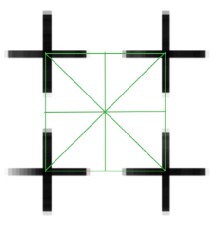
Refer to caption
Figure 15. The partition of the square [0,3]×[0,3][0,3]\times[0,3] into 88 triangles.
Lemma 4.18.

The smocking lengths are

Lm​i​n+\displaystyle L^{+}_{min} =\displaystyle= inf{L⁡(Ij):j∈J+}=2\displaystyle\inf\{L(I_{j}):\,j\in J_{+}\}=2 (4.49)
Lm​a​x+\displaystyle L^{+}_{max} =\displaystyle= sup{L⁡(Ij):j∈J+}=2\displaystyle\sup\{L(I_{j}):\,j\in J_{+}\}=2 (4.50)
Proof.

This follows from the fact that the diameter of a ++ shaped stitch IjI_{j} is 22. ∎

Lemma 4.19.

The smocking separation factor of (X+,d+)(X_{+},d_{+}) is

δ+=1\delta_{+}=1 (4.51)
Proof.

Notice the stitches I(0,0)I_{(0,0)} and I(3,0)I_{(3,0)} are a distance 11 apart and the stitches I(0,0)I_{(0,0)} and I(3,3)I_{(3,3)} are a distance 22+22=8\sqrt{2^{2}+2^{2}}=\sqrt{8} apart. By the symmetry of X+X_{+}, δ+=1\delta_{+}=1. ∎

4.6. The Smocking Constants of XHX_{H} by Victoria, Maziar, and Ajmain:

Here we find the smocking constants for XHX_{H}:

Lemma 4.20.

The smocking depth

hH=inf{r:𝔼2⊂Tr​(S)}∈[0,∞]=1.5h_{H}=\inf\{r:\,\mathbb{E}^{2}\subset T_{r}(S)\}\in[0,\infty]=1.5 (4.52)
Proof.

Note that the point (0,1.5)(0,1.5) is exactly distance 1.51.5 from the four stitches around it: I(0,0),I(0,3),I(−1.5,1.5),I_{(0,0)},I_{(0,3)},I_{(-1.5,1.5)}, and I(1.5,1.5)I_{(1.5,1.5)}). So hH≥1.5h_{H}\geq 1.5.

Now we must show 𝔼2⊂T1.5​(JH){\mathbb{E}}^{2}\subset T_{1.5}(J_{H}).

For each j∈J−j\in J_{-} let

□j=[j1−1.5,j1.+1.5]×[j2,j2+3],\square_{j}=[j_{1}-1.5,j_{1}.+1.5]\times[j_{2},j_{2}+3], (4.53)

which is a 3x3 square above IjI_{j} that touches I(j1,J2+3)I_{(j_{1},J_{2}+3)}, I(j1−1.5,j2+1.5)I_{(j_{1}-1.5,j_{2}+1.5)} or I(j1+1.5,j2+1.5)I_{(j_{1}+1.5,j_{2}+1.5)}. Let

⊞j\displaystyle\boxplus_{j} =\displaystyle= [j1−1.5,j1−0.5]×[j2,j2+1]\displaystyle[j_{1}-1.5,j_{1}-0.5]\times[j_{2},j_{2}+1]
⊔[j1+0.5,j1+1.5]×[j2,j2+1]\displaystyle\sqcup\,\,\,[j_{1}+0.5,j_{1}+1.5]\times[j_{2},j_{2}+1]
⊔[j1−1.5,j1−0.5]×[j2+2,j2+3]\displaystyle\sqcup\,\,\,[j_{1}-1.5,j_{1}-0.5]\times[j_{2}+2,j_{2}+3]
⊔[j1+0.5,j1+1.5]×[j2+2,j2+3].\displaystyle\sqcup\,\,\,[j_{1}+0.5,j_{1}+1.5]\times[j_{2}+2,j_{2}+3].

be four smaller unit squares in the corners of □j\square_{j}.

Notice

𝔼2=⋃j∈JH−□j=⋃j∈JH−⊞j⊔(□j∖⊞j).{\mathbb{E}}^{2}=\bigcup_{j\in J_{H}^{-}}\square_{j}=\bigcup_{j\in J_{H}^{-}}\boxplus_{j}\sqcup\left(\square_{j}\setminus\boxplus_{j}\right). (4.54)

Let (x,y)∈𝔼2(x,y)\in{\mathbb{E}}^{2}. Then there exists j∈JH−j\in J_{H}^{-} such that

(x,y)∈⊞j⊔(□j−⊞j).(x,y)\in\boxplus_{j}\sqcup\left(\square_{j}-\boxplus_{j}\right). (4.55)

Suppose (x,y)∈⊞j(x,y)\in\boxplus_{j}. Since ⊞j\boxplus_{j} is a disjoint union of four sets each with diameter 2\sqrt{2} and each intersecting SS, we know

(x,y)∈T2​(S)⊂T1.5​(S).(x,y)\in T_{\sqrt{2}}(S)\subset T_{1.5}(S). (4.56)

Suppose (x,y)∈□j−⊞j(x,y)\in\square_{j}-\boxplus_{j}. Note that

□j−⊞j\displaystyle\square_{j}-\boxplus_{j} =\displaystyle= [j1−0.5,j1+0.5]×[j2,j2+1.5]\displaystyle[j_{1}-0.5,j_{1}+0.5]\times[j_{2},j_{2}+1.5]
∪\displaystyle\cup [j1−0.5,j1+0,5]×[j2+1.5,j2+3]\displaystyle[j_{1}-0.5,j_{1}+0,5]\times[j_{2}+1.5,j_{2}+3]
∪\displaystyle\cup [j1,j1+1.5]×[j2+1,j2+2]\displaystyle[j_{1},j_{1}+1.5]\times[j_{2}+1,j_{2}+2]
∪\displaystyle\cup [j1−1.5,j1]×[j2+1,j2+2].\displaystyle[j_{1}-1.5,j_{1}]\times[j_{2}+1,j_{2}+2].

Therefore, (x,y)(x,y) is in at most a 1.51.5 distance from one of the stitches I(j1,j2)I_{(j_{1},j_{2})}, I(j1,J2+3)I_{(j_{1},J_{2}+3)}, I(j1−1.5,j2+1.5)I_{(j_{1}-1.5,j_{2}+1.5)} or I(j1+1.5,j2+1.5)I_{(j_{1}+1.5,j_{2}+1.5)}. Thus

(x,y)∈T1.5​(S).(x,y)\in T_{1.5}(S). (4.57)

∎

Lemma 4.21.

The smocking lengths are

L=Lm​i​nH=Lm​a​xH=1.L=L^{H}_{min}=L^{H}_{max}=1. (4.58)
Proof.

For each j∈Jj\in J we have L⁡(Ij)=1L(I_{j})=1. ∎

Lemma 4.22.

The smocking separation factor is

δH=2\delta_{H}=\sqrt{2} (4.59)
Proof.

By the translational and reflective symmetry of the H-smocking pattern,

δH=min{|z−w|:z∈I0,w∈Ij,j∈(J−{0})∩ℝ≥02}.\delta_{H}=\min\{|z-w|:z\in I_{0},w\in I_{j},j\in\left(J-\{0\}\right)\cap\mathbb{R}_{\geq 0}^{2}\}. (4.60)

Suppose j∈JH−∩ℝ+2j\in J_{H}^{-}\cap\mathbb{R}_{+}^{2}. Then

min{|v−w|:v∈I0,w∈Ij}=|(0.5,0)−(j1−0.5,j2)|≥|(0.5,0)−(3−0.5,3)|=13.\min\{|v-w|:v\in I_{0},w\in I_{j}\}=|(0.5,0)-(j_{1}-0.5,j_{2})|\geq|(0.5,0)-(3-0.5,3)|=\sqrt{13}.

Suppose j∈JH|∩ℝ+2j\in J_{H}^{|}\cap\mathbb{R}_{+}^{2}. Then

min{|v−w|:v∈I0,w∈Ij}=|(0.5,0)−(j1,j2−0.5)|≥|(0.5,0)−(1.5,1.5−0.5)|=2\min\{|v-w|:v\in I_{0},w\in I_{j}\}=|(0.5,0)-(j_{1},j_{2}-0.5)|\geq|(0.5,0)-(1.5,1.5-0.5)|=\sqrt{2}

Suppose j∈JH−∩({0}×ℝ+)j\in J_{H}^{-}\cap\left(\{0\}\times\mathbb{R}_{+}\right). Then

min{|v−w|:v∈I0,w∈Ij}=|(0,0)−(0,j2)|≥|(0,0)−(0,3)|=3.\min\{|v-w|:v\in I_{0},w\in I_{j}\}=|(0,0)-(0,j_{2})|\geq|(0,0)-(0,3)|=3.

Suppose j∈JH−∩(ℝ+×{0})j\in J_{H}^{-}\cap\left(\mathbb{R}_{+}\times\{0\}\right). Then

min{|v−w|:v∈I0,w∈Ij}=|(0.5,0)−(j1−0.5,0)|≥|(0.5,0)−(3−0.5,0)|=2.\min\{|v-w|:v\in I_{0},w\in I_{j}\}=|(0.5,0)-(j_{1}-0.5,0)|\geq|(0.5,0)-(3-0.5,0)|=2.

∎

4.7. The Smocking Constants of X□X_{\square} by Leslie, Emilio, and Aleah

Here we find the smocking constants for X□X_{\square}.

Lemma 4.23.

The smocking depth of X□X_{\square} is

h□=2h_{\square}=\sqrt{2} (4.61)
Proof.

By the symmetry of the square lattice we need only examine I(0,0),I(0,3),I(3,0),I(3,3)I_{(0,0)},I_{(0,3)},I_{(3,0)},I_{(3,3)} it is clear that the point simultaneously farthest from each square is (2,2)(2,2). It is 2\sqrt{2} distance from every square. ∎

Lemma 4.24.
Lm​i​n□\displaystyle L^{\square}_{min} =\displaystyle= inf{L⁡(Ij):j∈J□}=2\displaystyle\inf\{L(I_{j}):\,j\in J_{\square}\}=\sqrt{2} (4.62)
Lm​a​x□\displaystyle L^{\square}_{max} =\displaystyle= sup{L⁡(Ij):j∈J□}=2\displaystyle\sup\{L(I_{j}):\,j\in J_{\square}\}=\sqrt{2} (4.63)

so the smocking length is L□=2L_{\square}=\sqrt{2}.

Proof.

For X□X_{\square}, L⁡(Ij)=Diam⁡IjL(I_{j})=\operatorname{Diam}I_{j}. In this case of unit squares, it follows that L⁡(Ij)=2L(I_{j})=\sqrt{2}. ∎

Lemma 4.25.

The smocking separation factor is

δ□=2\delta_{\square}=2 (4.64)
Proof.

The minimum distance between any two squares is the plain Euclidean distance, which is 22. To prove this, we can use the symmetry of the pattern and compute any example. Consider the minimum distance between I(0,0)I_{(0,0)} and I(3,0)I_{(3,0)}, the distance would be the distance between (x1,y1)=(1,0)(x_{1},y_{1})=(1,0) and (x2,y2)=(3,0)(x_{2},y_{2})=(3,0) which is 22. ∎

5. Balls in Smocked Spaces

In this section we examine how balls in smocked spaces look by describing their preimages under the smocking map. We begin with a few useful lemmas and propositions about balls and then draw some of the balls in our smocked spaces in subsequent subsections.

5.1. Useful Facts about Balls in Smocked Spaces by Hindy and Moshe

Recall π:𝔼N→X\pi:\mathbb{E}^{N}\to X of Definition 3.1. In order to describe the balls in a smocked space precisely, we instead examine

π−1​(Br​(π⁡(p)))\displaystyle\pi^{-1}\left(B_{r}(\pi(p))\right) =\displaystyle= {x∈𝔼N:π⁡(x)∈Br​(π⁡(p))}\displaystyle\left\{x\in\mathbb{E}^{N}:\,\pi(x)\in B_{r}(\pi(p))\right\} (5.1)
=\displaystyle= {x∈𝔼N:d⁡(π⁡(x),π⁡(p))<r}\displaystyle\left\{x\in\mathbb{E}^{N}:\,d(\pi(x),\pi(p))<r\right\} (5.2)
=\displaystyle= {x∈𝔼N:d¯​(x,p)<r}.\displaystyle\left\{x\in\mathbb{E}^{N}:\,\bar{d}(x,p)<r\right\}. (5.3)

Our first lemma will be applied repeatedly within this section:

Lemma 5.1.

For all p∈𝔼Np\in{\mathbb{E}}^{N} and all r,s,>0r,s,>0 we have

Bs​(x)⊂π−1​(Bs​(π⁡(x))CLOSEB_{s}(x)\subset\pi^{-1}(B_{s}(\pi(x)) (5.4)

and

Ts​(π−1​(Br​(π⁡(x))))⊂π−1​(Br+s​(π⁡(x))).T_{s}(\pi^{-1}(B_{r}(\pi(x))))\subset\pi^{-1}(B_{r+s}(\pi(x))). (5.5)
Proof.

If v∈Bs​(x)v\in B_{s}(x) then |v−x|<s|v-x|<s so d⁡(π⁡(v),π⁡(x))<sd(\pi(v),\pi(x))<s which implies π⁡(v)∈Bs​(π⁡(x))\pi(v)\in B_{s}(\pi(x)) and we get (5.4). If v∈Ts​(π−1​(Br​(π⁡(x))))v\in T_{s}(\pi^{-1}(B_{r}(\pi(x)))), there exists z∈π−1​(Br​(π⁡(x)))z\in\pi^{-1}(B_{r}(\pi(x))) such that

d⁡(π⁡(v),π⁡(z))<s​ and ​d​(π⁡(z),π⁡(x))<r.d(\pi(v),\pi(z))<s\textrm{ and }d(\pi(z),\pi(x))<r. (5.6)

Then by the triangle inequality,

d⁡(π⁡(v),π⁡(x))≤d⁡(π⁡(v),π⁡(z))+d⁡(π⁡(z),π⁡(x))<s+r.d(\pi(v),\pi(x))\leq d(\pi(v),\pi(z))+d(\pi(z),\pi(x))<s+r. (5.7)

It follows that v∈π−1​(Br+s​(π⁡(x))).v\in\pi^{-1}(B_{r+s}(\pi(x))). ∎

In our first proposition we examine a small ball about a stitch point whose radius is less than the separation factor of the smocked space:

Proposition 5.2.

Suppose that IjI_{j} is a smocking stitch and r<δXr<\delta_{X} as defined in Definition 4.6, then

π−1​(Br​(π⁡(Ij)))=Tr​(Ij)\pi^{-1}(B_{r}(\pi(I_{j})))=T_{r}(I_{j}) (5.8)
Proof.

For each v∈Tr​(Ij),v\in T_{r}(I_{j}), there exists some z∈Ijz\in I_{j} such that |v−z|<r.|v-z|<r. Therefore,

d⁡(π⁡(v),π⁡(Ij))≤d0​(v,z)=|v−z|<rd(\pi(v),\pi(I_{j}))\leq d_{0}(v,z)=|v-z|<r (5.9)

so v∈π−1​(Br​(π⁡(Ij))).v\in\pi^{-1}(B_{r}(\pi(I_{j}))).

To prove the converse, consider v∈π−1​(Br​(π⁡(Ij))).v\in\pi^{-1}(B_{r}(\pi(I_{j}))). Setting p=π⁡(v)p=\pi(v) we have d⁡(p,π⁡(Ij))<r.d(p,\pi(I_{j}))<r. This implies that

d(p,π(Ij))=min{d0(y,y′),d1(y,y′):y∈π−1(p),y′∈Ij}d(p,\pi(I_{j}))=\min\{d_{0}(y,y^{\prime}),d_{1}(y,y^{\prime}):\,y\in\pi^{-1}(p),\,\,y^{\prime}\in I_{j}\} (5.10)

since

dn​(y,y′)≥δX>r​ for ​n≥2.d_{n}(y,y^{\prime})\geq\delta_{X}>r\textrm{ for }n\geq 2. (5.11)

By definition,

d1(y,y′)=min{|y−z1|+|z1′−y′|:z1,z1′∈Ik}d_{1}(y,y^{\prime})=\min\{|y-z_{1}|+|z^{\prime}_{1}-y^{\prime}|:\,z_{1},z_{1}^{\prime}\in I_{k}\} (5.12)

for some Ik.I_{k}. If d1​(y,y′)<r<δXd_{1}(y,y^{\prime})<r<\delta_{X}, then Ik=IjI_{k}=I_{j}, so it follows that

d1​(y,y′)≥min⁡{|y−z1|:z1∈Ij}=d0​(y,y′).d_{1}(y,y^{\prime})\geq\min\{|y-z_{1}|\ :z_{1}\in I_{j}\}=d_{0}(y,y^{\prime}). (5.13)

But also

d1​(y,y′)≤min⁡{|y−z1|+|y′−y′|:z1∈Ij}=d0​(y,y′)d_{1}(y,y^{\prime})\leq\min\{|y-z_{1}|+|y^{\prime}-y^{\prime}|\ :z_{1}\in I_{j}\}=d_{0}(y,y^{\prime}) (5.14)

Therefore

d⁡(p,π⁡(Ij))\displaystyle d(p,\pi(I_{j})) =\displaystyle= min{d0(y,y′):y∈π−1(p),y′∈Ij}\displaystyle\min\{d_{0}(y,y^{\prime}):\,y\in\pi^{-1}(p),\,y^{\prime}\in I_{j}\} (5.15)
=\displaystyle= min{|y−y′|:y∈π−1(p),y′∈Ij}\displaystyle\min\{|y-y^{\prime}|:\,y\in\pi^{-1}(p),\,y^{\prime}\in I_{j}\} (5.16)

So

∃y′∈Ij​∃y∈π−1​(p)​ such that ​|y−y′|<r.\exists y^{\prime}\in I_{j}\,\exists y\in\pi^{-1}(p)\textrm{ such that }|y-y^{\prime}|<r. (5.17)

Since r<δXr<\delta_{X}, it follows that y∉Sy\notin S. Thus

π⁡(v)=p=π⁡(y)∉π⁡(S).\pi(v)=p=\pi(y)\notin\pi(S). (5.18)

Therefore, v=yv=y, and

∃y′∈Ij​ such that ​|v−y′|<r.\exists y^{\prime}\in I_{j}\textrm{ such that }|v-y^{\prime}|<r. (5.19)

So v∈Tr​(Ij)v\in T_{r}(I_{j}). ∎

Proposition 5.3.

Suppose that x∈𝔼N∖Sx\in{\mathbb{E}}^{N}\setminus S and r<D⁡(x)r<D(x) is defined as in Definition 4.6, then

π−1​(Br​(π⁡(x)))=Br​(x)={y:|x−y|<r}.\pi^{-1}(B_{r}(\pi(x)))=B_{r}(x)=\{y:\,|x-y|<r\}. (5.20)
Proof.

Note that v∈π−1​(Br​(π⁡(x)))v\in\pi^{-1}(B_{r}(\pi(x))) iff π⁡(v)∈Br​(π⁡(x)).\pi(v)\in B_{r}(\pi(x)). By the definition of the smocking distance, this is true iff

min⁡{d0​(π⁡(v),π⁡(x)),d1​(π⁡(v),π⁡(x)),d2​(π⁡(v),π⁡(x)),…}=d⁡(π⁡(v),π⁡(x))<r<D⁡(x).\min\{d_{0}(\pi(v),\pi(x)),d_{1}(\pi(v),\pi(x)),d_{2}(\pi(v),\pi(x)),...\}=d(\pi(v),\pi(x))<r<D(x). (5.21)

By the hypothesis |z−x|≥D⁡(x)∀z∈S|z-x|\geq D(x)\quad\forall z\in S, so by the definition of smocking distance for all j≥1j\geq 1

dj​(π⁡(v),π⁡(x))≥min⁡{|z−x|:z∈S}≥D⁡(x).d_{j}(\pi(v),\pi(x))\geq\min\{|z-x|:\,z\in S\}\geq D(x). (5.22)

Thus the minimum in (5.21) is achieved by

d0​(π⁡(v),π⁡(x))=d⁡(π⁡(v),π⁡(x))<r<D⁡(x).d_{0}(\pi(v),\pi(x))=d(\pi(v),\pi(x))<r<D(x). (5.23)

So (5.21) holds iff |v−x|<r|v-x|<r which is true iff x∈Br​(p)x\in B_{r}(p). ∎

In our next proposition we explore how a ball grows when there are no smocking stitches too close to the original ball:

Proposition 5.4.

Suppose that the points in the smocking set are a definite distance,

δr=min{|z−w|:z∈S∖π−1(Br(π(p))),w∈π−1(Br(π(p)))}>0,\delta_{r}=\min\left\{|z-w|:\,\,z\in S\,\setminus\pi^{-1}(B_{r}(\pi(p))),\,\,w\in\pi^{-1}(B_{r}(\pi(p)))\right\}>0, (5.24)

away from the points within the ball. Then for all r>0r>0 and for all s∈(0,δr]s\in(0,\delta_{r}]

π−1​(Br+s​(π⁡(x)))=Ts​(π−1​(Br​(π⁡(x))))\pi^{-1}\bigg(B_{r+s}(\pi(x))\bigg)=T_{s}\bigg(\pi^{-1}(B_{r}(\pi(x)))\bigg) (5.25)
Proof.

Suppose v∈π−1​(Br+s​(π⁡(x))).v\in\pi^{-1}(B_{r+s}(\pi(x))). If x∈π−1​(Br​(π⁡(x)))x\in\pi^{-1}(B_{r}(\pi(x))) then clearly

v∈Ts​(π−1​(Br​(π⁡(x)))),v\in T_{s}\left(\pi^{-1}(B_{r}(\pi(x)))\right), (5.26)

and we are done. If not, note that the distance d⁡(π⁡(v),π⁡(x))<r+s,d(\pi(v),\pi(x))<r+s, is achieved by a collection of segments starting at y∈π−1​(π​(v))y\in\pi^{-1}(\pi(v)) and ending at y′∈π−1​(π⁡(x))y^{\prime}\in\pi^{-1}(\pi(x)):

d⁡(π⁡(v),π⁡(x))=|y−z1|+∑i=1n|zi′−zi+1|+|zk′−y′|d(\pi(v),\pi(x))=|y-z_{1}|+\sum_{i=1}^{n}|z^{\prime}_{i}-z_{i+1}|+|z^{\prime}_{k}-y^{\prime}| (5.27)

for some n≥0n\geq 0, where π⁡(zi)=π⁡(zi′)\pi(z_{i})=\pi(z^{\prime}_{i}) for each ii. Notice that for any zi′z_{i}^{\prime} in the minimizing sum, we must have

d⁡(π⁡(v),π⁡(x))=d⁡(π⁡(v),π⁡(zi′))+d⁡(π⁡(zi′),π⁡(x)),d(\pi(v),\pi(x))=d(\pi(v),\pi(z_{i}^{\prime}))+d(\pi(z_{i}^{\prime}),\pi(x)), (5.28)

Since y∉π−1​(Br​(π⁡(x)))y\notin\pi^{-1}(B_{r}(\pi(x))) and y′∈π−1​(Br​(π⁡(x))),y^{\prime}\in\pi^{-1}(B_{r}(\pi(x))), at least one term in the sum must be of the form |a−b||a-b| where a∉π−1​(Br​(π⁡(x)))a\notin\pi^{-1}(B_{r}(\pi(x))) and b∈π−1​(Br​(π⁡(x))).b\in\pi^{-1}(B_{r}(\pi(x))). Since d¯​(a,x)>r\bar{d}(a,x)>r and d¯​(b,x)<r,\bar{d}(b,x)<r, the line segment from aa to bb must hit a point cc such that d¯​(c,p)=d⁡(π⁡(c),π⁡(x))=r,\bar{d}(c,p)=d(\pi(c),\pi(x))=r, by the continuity of the pseudometric d¯\bar{d}. It follows that

r+s\displaystyle r+s >\displaystyle> dn​(y,y′)\displaystyle d_{n}(y,y^{\prime}) (5.29)
≥\displaystyle\geq d⁡(π⁡(a),π⁡(x))\displaystyle d(\pi(a),\pi(x)) (5.30)
=\displaystyle= |a−b|+d⁡(π⁡(b),π⁡(x))\displaystyle|a-b|+d(\pi(b),\pi(x)) (5.31)
=\displaystyle= |a−c|+|c−b|+d⁡(π⁡(b),π⁡(x))\displaystyle|a-c|+|c-b|+d(\pi(b),\pi(x)) (5.32)
=\displaystyle= |a−c|+d⁡(π⁡(c),π⁡(x))\displaystyle|a-c|+d(\pi(c),\pi(x)) (5.33)
=\displaystyle= |a−c|+r.\displaystyle|a-c|+r. (5.34)

This implies that |a−c|<s.|a-c|<s. If a∈Sa\in S then |a−c|≥δr≥s|a-c|\geq\delta_{r}\geq s, which is a contradiction. Therefore, a∉Sa\notin S which implies that a=v.a=v. Hence, |v−c|<s|v-c|<s which implies that

v∈Ts​(π−1​(Br​(π⁡(x)))¯)=Ts​(π−1​(Br​(π⁡(x)))).v\in T_{s}\left(\,\overline{\pi^{-1}(B_{r}(\pi(x)))}\,\right)=T_{s}\left(\pi^{-1}(B_{r}(\pi(x)))\right). (5.35)

The other direction holds by Lemma 5.1. ∎

Lemma 5.5.

In a smocked metric space as in Definition 3.1. If there is a stitch, IjI_{j} such that

π−1​(B¯r​(π⁡(x)))∩Ij≠∅\pi^{-1}(\bar{B}_{r}(\pi(x)))\cap I_{j}\neq\emptyset (5.36)

then for all s>0s>0

Ts​(π−1​(Br​(π⁡(x))))∪Ts​(I)⊂π−1​(Br+s​(π⁡(x)))T_{s}\bigg(\pi^{-1}(B_{r}(\pi(x)))\bigg)\cup T_{s}(I)\subset\pi^{-1}\bigg(B_{r+s}(\pi(x))\bigg) (5.37)
Proof.

For each v∈Ts​(Ij),v\in T_{s}(I_{j}), there exists some z∈Ijz\in I_{j} such that |v−z|<s.|v-z|<s. Therefore,

d⁡(π⁡(v),π⁡(Ij))≤d0​(v,z)=|v−z|<sd(\pi(v),\pi(I_{j}))\leq d_{0}(v,z)=|v-z|<s (5.38)

so

Ts​(Ij)⊂π−1​(Bs​(π⁡(Ij))).T_{s}(I_{j})\subset\pi^{-1}(B_{s}(\pi(I_{j}))). (5.39)

By assumption we have

π⁡(Ij)∈B¯r​(π⁡(x))\pi(I_{j})\in\bar{B}_{r}(\pi(x)) (5.40)

which gives us

Bs​(π⁡(Ij))⊂Br+s​(π⁡(x)).B_{s}(\pi(I_{j}))\subset B_{r+s}(\pi(x)). (5.41)

By looking at the preimages we get

π−1​(Bs​(π⁡(Ij)))⊂π−1​(Br+s​(π⁡(x))).\pi^{-1}(B_{s}(\pi(I_{j})))\subset\pi^{-1}(B_{r+s}(\pi(x))). (5.42)

Combining this with line 5.39 we get

Ts​(Ij)⊂π−1​(Bs​(π⁡(Ij)))⊂π−1​(Br+s​(π⁡(x))).T_{s}(I_{j})\subset\pi^{-1}(B_{s}(\pi(I_{j})))\subset\pi^{-1}(B_{r+s}(\pi(x))). (5.43)

In order to show that

Ts​(π−1​(Br​(π⁡(x))))⊂π−1​(Br+s​(π⁡(p)))T_{s}(\pi^{-1}(B_{r}(\pi(x))))\subset\pi^{-1}(B_{r+s}(\pi(p))) (5.44)

we apply Lemma 5.1. ∎

Proposition 5.6.

If we consider all the smocking stitches that just touch a given ball:

Jr={j∈J:Ij∩π−1​(B¯r​(x))≠∅​ and ​Ij∩π−1​(Br​(x))=∅}J_{r}=\left\{j\in J:\,\,I_{j}\cap\pi^{-1}(\bar{B}_{r}(x))\neq\emptyset\textrm{ and }I_{j}\cap\pi^{-1}(B_{r}(x))=\emptyset\right\} (5.45)

and the distance to the nearest smocking interval that does not touch this ball

δ¯r=min{|z−w|:z∈S∖π−1(B¯r(π(v))),w∈π−1(B¯r(π(v)))}>0,\bar{\delta}_{r}=\min\left\{|z-w|:\,\,z\in S\,\setminus\pi^{-1}(\bar{B}_{r}(\pi(v))),\,\,w\in\pi^{-1}(\bar{B}_{r}(\pi(v)))\right\}>0, (5.46)

then for all s≤δ¯rs\leq\bar{\delta}_{r} we have

π−1​(Br+s​(π⁡(v)))=Ts​(π−1​(Br​(π⁡(v))))∪⋃j∈JrTs​(Ij).\pi^{-1}(B_{r+s}(\pi(v)))=T_{s}\left(\pi^{-1}(B_{r}(\pi(v)))\right)\cup\bigcup_{j\in J_{r}}T_{s}(I_{j}). (5.47)
Proof.

By applying Lemma 5.5 to each j∈Jrj\in J_{r} we know that

Ts​(π−1​(Br​(π⁡(v))))∪⋃j∈JrTs​(Ij)⊂π−1​(Br+s​(π⁡(v))).T_{s}\left(\pi^{-1}(B_{r}(\pi(v)))\right)\cup\bigcup_{j\in J_{r}}T_{s}(I_{j})\subset\pi^{-1}(B_{r+s}(\pi(v))). (5.48)

So we need only show that

π−1​(Br+s​(π⁡(v)))⊂Ts​(π−1​(Br​(π⁡(v))))∪⋃j∈JrTs​(Ij).\pi^{-1}(B_{r+s}(\pi(v)))\subset T_{s}\left(\pi^{-1}(B_{r}(\pi(v)))\right)\cup\bigcup_{j\in J_{r}}T_{s}(I_{j}). (5.49)

We want to show that for any q∈Br+s​(π​(v))q\in B_{r+s}(\pi(v)), that one of the following holds:

(A)\displaystyle(A)\qquad ∃x′∈π−1​(Br​(π⁡(v)))\displaystyle\exists x^{\prime}\in\pi^{-1}(B_{r}(\pi(v))) such that ​|x′−π−1​(q)|<s\displaystyle\textrm{ such that }|x^{\prime}-\pi^{-1}(q)|<s
(B)\displaystyle(B)\qquad ∃j∈Jr,z∈Ij\displaystyle\exists j\in J_{r},\,\,z\in I_{j} such that ​|z−π−1​(q)|<s.\displaystyle\textrm{such that }|z-\pi^{-1}(q)|<s.

First, consider q∈(Br+s​(π⁡(v)))∩π⁡(S)q\in(B_{r+s}(\pi(v)))\cap\pi(S). Since s<δ¯rs<\bar{\delta}_{r} all of the smocking intervals intersecting with π−1​(Br+s​(π⁡(v)))\pi^{-1}(B_{r+s}(\pi(v))) must either be contained inside π−1​(B¯r​(π⁡(v)))\pi^{-1}(\bar{B}_{r}(\pi(v))) in which case (A) holds, or be one of the IjI_{j} for some j∈Jrj\in J_{r} in which case (B) holds.

Now consider q∈(Br+s​(π⁡(v)))∖π⁡(S)q\in(B_{r+s}(\pi(v)))\setminus\pi(S), which implies there exists a unique point y∈𝔼Ny\in{\mathbb{E}}^{N} such that

π⁡(y)=q​ and ​d​(p,π⁡(v))=d⁡(π⁡(y),π⁡(v))<r+s.\pi(y)=q\textrm{ and }d(p,\pi(v))=d(\pi(y),\pi(v))<r+s. (5.50)

Since δX>0\delta_{X}>0, by Theorem 3.3 we know that one of the following cases holds:

Case I: d⁡(p,π⁡(v))=d⁡(π⁡(y),π⁡(v))=|v−y|\displaystyle d(p,\pi(v))=d(\pi(y),\pi(v))=|v-y|
Case II: ∃Ij∈S​∃w,w′∈Ij​s.t.d⁡(q,π⁡(v))=d⁡(π⁡(y),π⁡(v))=|y−w|+|w′−v|.\displaystyle\exists\,I_{j}\in S\,\,\exists\,w,w^{\prime}\in I_{j}\,s.t.\,\,\,d(q,\pi(v))=d(\pi(y),\pi(v))=|y-w|+|w^{\prime}-v|.

In Case I we see that

y∈Ts​(Br​(v))⊂Ts​(π−1​(Br​(π⁡(v))))y\in T_{s}(B_{r}(v))\subset T_{s}(\pi^{-1}(B_{r}(\pi(v)))) (5.51)

by Lemma 5.1. So we have (A) because

∃x′∈π−1​(Br​(π⁡(v)))​ such that ​|x′−π−1​(q)|=|x′−y|<s.\exists x^{\prime}\in\pi^{-1}(B_{r}(\pi(v)))\textrm{ such that }|x^{\prime}-\pi^{-1}(q)|=|x^{\prime}-y|<s. (5.52)

In Case II,

∃Ij∈S​w,w′∈Ij​s.t.d⁡(q,π⁡(v))=d⁡(π⁡(y),π⁡(v))=|y−w|+|w′−v|<r+s\exists I_{j}\in S\,\,w,w^{\prime}\in I_{j}\,s.t.\,d(q,\pi(v))=d(\pi(y),\pi(v))=|y-w|+|w^{\prime}-v|<r+s (5.53)

and the interval IjI_{j} intersects with Br​(π​(v))B_{r}(\pi(v)), so Ij∈Br​(π⁡(v))I_{j}\in B_{r}(\pi(v)). Consider the point z∈B¯r​(π​(p))z\in\bar{B}_{r}(\pi(p)) which minimizes d⁡(q,z)d(q,z). Since the closest smocking interval lies inside Br​(π​(v))B_{r}(\pi(v)) we know that zz is either inside Br​(π​(v))B_{r}(\pi(v)) (in which case yy is as well) or zz is on the boundary. In the second case d⁡(p,z)=rd(p,z)=r so

d⁡(q,z)=|y−π−1​(z)|<s.d(q,z)=|y-\pi^{-1}(z)|<s. (5.54)

If the interval IjI_{j} does not intersect with Br​(π​(p))B_{r}(\pi(p)) then it must be in JrJ_{r}. Then since

d⁡(q,π⁡(v))=d⁡(q,Ij)+d⁡(Ij,π⁡(v))<r+sd(q,\pi(v))=d(q,I_{j})+d(I_{j},\pi(v))<r+s (5.55)

and d⁡(Ij,π⁡(v))=rd(I_{j},\pi(v))=r we have d⁡(q,Ij)<sd(q,I_{j})<s which gives us that π−1​(q)∈Ts​(Ij)\pi^{-1}(q)\in T_{s}(I_{j})and so we have completed the proof of (B). ∎

5.2. Exploring the Balls in X⋄X_{\diamond} by Prof. Sormani and Dr. Kazaras:

Here we consider balls in X⋄X_{\diamond} centered on the point,

p0=I(0,0)=[−1/2,1/2]×{0},p_{0}=I_{(0,0)}=[-1/2,1/2]\times\{0\}, (5.56)

by drawing their preimages π−1​(BR​(p0))⊂𝔼N\pi^{-1}(B_{R}(p_{0}))\subset{\mathbb{E}}^{N}. See Figure 16.

Refer to caption
Figure 16. Lifts of balls, BR​(p0)B_{R}(p_{0}), where p0=I(0,0)p_{0}=I_{(0,0)} in the smocked space (X⋄,d⋄)(X_{\diamond},d_{\diamond}).

Observe that by Lemma 5.2 we know that

π−1​(BR​(p0))=TR​(I(0,0))∀R∈(0,1],\pi^{-1}(B_{R}(p_{0}))=T_{R}(I_{(0,0)})\quad\forall R\in(0,1], (5.57)

because the smocking separation factor was proven in Lemma 4.10 to be δ⋄=1.\delta_{\diamond}=1. Thus the ball of radius R=1/2R=1/2 is depicted in red and of radius R=1R=1 is depicted in orange in Figure 16.

We next apply Proposition 5.6, keeping in mind that δ⋄=1\delta_{\diamond}=1 and observing that when r=1r=1 there are six stitches touching the ball of radius r=1r=1. This gives us the ball of radius 3/23/2 depicted in yellow in Figure 16:

π−1​(B3/2​(p))=T1/2​(π−1​(B1​(p)))∪⋃j∈J1T1/2​(Ij)\pi^{-1}(B_{3/2}(p))=T_{1/2}\left(\pi^{-1}(B_{1}(p))\right)\cup\bigcup_{j\in J_{1}}T_{1/2}(I_{j}) (5.58)

where

J1={(1,1),(2,0),(1,−1),(−1,−1),(−2,0),(−1,1)}.J_{1}=\{(1,1),(2,0),(1,-1),(-1,-1),(-2,0),(-1,1)\}. (5.59)

We then apply Proposition 5.4 with r=3/2r=3/2 and s=1/2s=1/2 to find the ball of radius 22 depicted in green in Figure 16:

π−1​(B2​(p))=T1/2​(π−1​(B3/2​(p))).\pi^{-1}(B_{2}(p))=T_{1/2}(\pi^{-1}(B_{3/2}(p))). (5.60)

We next apply Proposition 5.6, observing that when r=2r=2 there are twelve stitches touching the ball of radius r=2r=2:

J2={(0,±2),(±2,±2),(±3,±1),(±4,±0)}.J_{2}=\{(0,\pm 2),(\pm 2,\pm 2),(\pm 3,\pm 1),(\pm 4,\pm 0)\}. (5.61)

This gives us the ball of radius 5/25/2 depicted in pale green in Figure 16:

π−1​(B5/2​(p))=T1/2​(π−1​(B2​(p)))∪⋃j∈J2T1/2​(Ij).\pi^{-1}(B_{5/2}(p))=T_{1/2}\left(\pi^{-1}(B_{2}(p))\right)\cup\bigcup_{j\in J_{2}}T_{1/2}(I_{j}). (5.62)

We continue in this matter to complete the drawing in Figure 16 by eye.

While it can be rather complicated to provide formulas for these sets, we can nevertheless approximately describe their shapes. For large radii, these balls appear to have a hexagonal shape to them. In fact it appears approximately to be the intersection of the strip, y−1​(−r,r)y^{-1}(-r,r) with the diamond:

{(x,y):|x|+|y|<R}​ which has vertices at ​(±R,0)​ and ​(0,±R)\{(x,y):\,\,|x|+|y|<R\}\textrm{ which has vertices at }(\pm R,0)\textrm{ and }(0,\pm R) (5.63)

where R=2​rR=2r. There is an error in this approximation of about the length of a smocking interval.

We conjecture that Jr=J¯r∪J^rJ_{r}=\bar{J}_{r}\cup\hat{J}_{r} where

J¯r\displaystyle\bar{J}_{r} =\displaystyle= {(j1,j2)∈J⋄:|j2|=r​ and ​|j1|≤|j2|}\displaystyle\{(j_{1},j_{2})\in J_{\diamond}:\,\,|j_{2}|=r\textrm{ and }|j_{1}|\leq|j_{2}|\}
J^r\displaystyle\hat{J}_{r} =\displaystyle= {(j1,j2)∈J⋄:|j1+j2|∈[2​r−1,2​r]}\displaystyle\{(j_{1},j_{2})\in J_{\diamond}:\,\,|j_{1}+j_{2}|\in[2r-1,2r]\}

Due to the lengthiness of the proof required to rigorously prove this guess is true, we postpone studying this particular smocked space further in this paper. See [8] for a rigorous study of this space.

5.3. Exploring the Balls in XTX_{T} by Julinda, Aleah, and Victoria

Here we consider balls in XTX_{T} centered on the point,

p0=I(0,0)=[−1,1]×{0},p_{0}=I_{(0,0)}=[-1,1]\times\{0\}, (5.64)

by drawing their preimages π−1​(BR​(p0))⊂𝔼N\pi^{-1}(B_{R}(p_{0}))\subset{\mathbb{E}}^{N}. See Figure 17.

Refer to caption
Figure 17. Lifts of balls, BR​(p0)B_{R}(p_{0}), where p0=I(0,0)p_{0}=I_{(0,0)} in the smocked space (XT,dT)(X_{T},d_{T}).

Observe that by Lemma 5.2 we know that

π−1​(BR​(p0))=TR​(I(0,0))∀R∈(0,1],\pi^{-1}(B_{R}(p_{0}))=T_{R}(I_{(0,0)})\quad\forall R\in(0,1], (5.65)

because the smocking separation factor was proven in Lemma 4.16 to be δ⋄=1.\delta_{\diamond}=1. Thus the ball of radius R=1R=1 is depicted in red in Figure 17.

We next apply Proposition 5.6, keeping in mind that δT=1\delta_{T}=1 and observing that when r=1r=1 there are four stitches touching the ball of radius r=1r=1. This gives us the ball of radius 22 depicted in orange in Figure 17:

π−1​(B2​(p))=T1/2​(π−1​(B1​(p)))∪⋃j∈J1T1​(Ij)\pi^{-1}(B_{2}(p))=T_{1/2}\left(\pi^{-1}(B_{1}(p))\right)\cup\bigcup_{j\in J_{1}}T_{1}(I_{j}) (5.66)

where

J1={(2,0),(0,2),(−2,0),(0,−2)}.J_{1}=\{(2,0),(0,2),(-2,0),(0,-2)\}. (5.67)

We next apply Proposition 5.6, observing that when r=3r=3 there are eight stitches touching the ball of radius r=2r=2:

J2={(0,±4),(±2,±2),(±4,±0)}.J_{2}=\{(0,\pm 4),(\pm 2,\pm 2),(\pm 4,\pm 0)\}. (5.68)

This gives us the ball of radius 33 depicted in yellow in Figure 17:

π−1​(B3​(p))=T1​(π−1​(B2​(p)))∪⋃j∈J2T1​(Ij).\pi^{-1}(B_{3}(p))=T_{1}\left(\pi^{-1}(B_{2}(p))\right)\cup\bigcup_{j\in J_{2}}T_{1}(I_{j}). (5.69)

We continue in this matter to easily complete the drawing in Figure 17.

A rigorous analysis of this space will be continued within this paper.

5.4. Exploring the Balls in X=X_{=} by Prof. Sormani, Leslie, and Shanell

Here we consider balls in X=X_{=} centered on the point,

p0=I(0,0)=[−.5,.5]×{0},p_{0}=I_{(0,0)}=[-.5,.5]\times\{0\}, (5.70)

by drawing their preimages π−1​(BR​(p0))⊂𝔼N\pi^{-1}(B_{R}(p_{0}))\subset{\mathbb{E}}^{N}. See Figure 18.

Refer to caption
Figure 18. Lifts of balls, BR​(p0)B_{R}(p_{0}), where p0=I(0,0)p_{0}=I_{(0,0)} in the smocked space (X=,d=)(X_{=},d_{=})..

By Proposition 5.2 we know that

π−1​(BR​(p0))=TR​(I(0,0))∀R∈(0,1],\pi^{-1}(B_{R}(p_{0}))=T_{R}(I_{(0,0)})\quad\forall R\in(0,1], (5.71)

because the smocking separation factor was proven in Lemma 4.16 to be δ⋄=1.\delta_{\diamond}=1. Thus the ball of radius R=1R=1 is depicted in red in Figure 18.

To find the ball of radius 22 depicted in orange in Figure  observe that we need to do things very carefully. Proposition 5.6 implies that

π−1​(B1+s​(π⁡(p)))=Ts​(π−1​(B1​(π⁡(p))))∪⋃j∈J1Ts​(Ij)\pi^{-1}(B_{1+s}(\pi(p)))=T_{s}\left(\pi^{-1}(B_{1}(\pi(p)))\right)\cup\bigcup_{j\in J_{1}}T_{s}(I_{j}) (5.72)

where

J1={(2,0),(0,2),(−2,0),(0,−2)}J_{1}=\{(2,0),(0,2),(-2,0),(0,-2)\} (5.73)

and

s≤δr¯=2−1s\leq\bar{\delta_{r}}=\sqrt{2}-1 (5.74)

because at 2\sqrt{2} we hit the intervals in

J2={±2,±2}.J_{\sqrt{2}}=\{\pm 2,\pm 2\}. (5.75)

So

π−1​(B2​(p))=T1​(π−1​(B1​(p)))∪⋃j∈J1T1​(Ij)∪⋃j∈J2T2−2​(Ij).\pi^{-1}(B_{2}(p))=T_{1}\left(\pi^{-1}(B_{1}(p))\right)\cup\bigcup_{j\in J_{1}}T_{1}(I_{j})\cup\bigcup_{j\in J_{\sqrt{2}}}T_{2-\sqrt{2}}(I_{j}). (5.76)

To find the ball of radius 33 we need

J3={(±3,0),(0,±3)}​ and ​J5={±1,±2}​ and ​J1+2={±2,±1}J_{3}=\{(\pm 3,0),(0,\pm 3)\}\textrm{ and }J_{\sqrt{5}}=\{\pm 1,\pm 2\}\textrm{ and }J_{1+\sqrt{2}}=\{\pm 2,\pm 1\} (5.77)

so we see that things become very complicated rapidly. Nevertheless we roughly draw the balls by eye using an art program to produce Figure 18.

Although these balls appear to be converging to an ellipse, this has been shown to be false. Due to the lengthy nature of the estimates involved we will not explore X=X_{=} further within this paper. Further work on this space will appear in [8].

5.5. Exploring the Balls in X+X_{+} by Emilio, Moshe, and Ajmain

Let us consider balls in X+X_{+} around

p0=I(0,0)=([−1,1]×{(0,0)})∪({(0,0)}×[−1,1])p_{0}=I_{(0,0)}=([-1,1]\times\{(0,0)\})\cup(\{(0,0)\}\times[-1,1]) (5.78)

by drawing their preimages π−1​(BR​(p0))⊂𝔼N\pi^{-1}(B_{R}(p_{0}))\subset{\mathbb{E}}^{N}. See Figure 19.

Refer to caption
Figure 19. Lifts of balls, BR​(p0)B_{R}(p_{0}), where p0=I(0,0)p_{0}=I_{(0,0)} in the smocked space (X+,d+)(X_{+},d_{+}).

Observe that by Lemma 5.2 we know that

π−1​(BR​(p0))=TR​(I(0,0))∀R∈(0,1],\pi^{-1}(B_{R}(p_{0}))=T_{R}(I_{(0,0)})\quad\forall R\in(0,1], (5.79)

because the smocking separation factor was proven in Lemma 4.19 to be δ+=1.\delta_{+}=1. Thus the ball of radius R=1R=1 is depicted in red in Figure 19.

We next apply Proposition 5.6, keeping in mind that δT=1\delta_{T}=1 and observing that when r=1r=1 there are four stitches touching the ball of radius r=1r=1. This gives us the ball of radius 22 depicted in orange in Figure 19:

π−1​(B2​(p))=T1/2​(π−1​(B1​(p)))∪⋃j∈J1T1​(Ij)\pi^{-1}(B_{2}(p))=T_{1/2}\left(\pi^{-1}(B_{1}(p))\right)\cup\bigcup_{j\in J_{1}}T_{1}(I_{j}) (5.80)

where

J1={(±3,0),(0,±3)}.J_{1}=\{(\pm 3,0),(0,\pm 3)\}. (5.81)

We next apply Proposition 5.6 again, observing that when r=3r=3 there are eight stitches touching the ball of radius r=2r=2:

Jr={(0,±6),(±3,±3),(±6,±0)}.J_{r}=\{(0,\pm 6),(\pm 3,\pm 3),(\pm 6,\pm 0)\}. (5.82)

This gives us the ball of radius 33 depicted in yellow in Figure 19:

π−1​(B3​(p))=T1​(π−1​(B2​(p)))∪⋃j∈J2T1​(Ij).\pi^{-1}(B_{3}(p))=T_{1}\left(\pi^{-1}(B_{2}(p))\right)\cup\bigcup_{j\in J_{2}}T_{1}(I_{j}). (5.83)

We continue in this matter to complete the drawing in Figure 19.

Remark 5.7.

It appears that the balls are bumpy diamond shapes. That is if k=⌈r⌉k=\lceil{r}\rceil, with r>1r>1 then

S3​(k−2)′⊂π−1​(Br​(p))⊂S3​k′,S^{\prime}_{3(k-2)}\subset\pi^{-1}(B_{r}(p))\subset S^{\prime}_{3k}, (5.84)

where

Sr′={x∈X+:dT​(x,p)<r}S^{\prime}_{r}=\{x\in X_{+}\,:\,d_{T}(x,p)<r\} (5.85)

with dTd_{T} being the taxicab metric:

dT​(x,y)=|x1−y1|+|x2−y2|d_{T}(x,y)=|x_{1}-y_{1}|+|x_{2}-y_{2}| (5.86)

where x=(x1,x2)x=(x_{1},x_{2}), y=(y1,y2)y=(y_{1},y_{2}).

Remark 5.8.

If k=⌈r⌉k=\lceil{r}\rceil, then we define Jr+J^{+}_{r} as such.

Jr+=J1+∪J2+∪⋯∪Jk−1+∪Jk+J^{+}_{r}=J^{+}_{1}\cup J^{+}_{2}\cup\dots\cup J^{+}_{k-1}\cup J^{+}_{k} (5.87)

where

Jk+={±(0,3​(k−1)),±(3⋅1,3​(k−2)),…,±(3⋅(k−1),0)}J^{+}_{k}=\{\pm(0,3(k-1)),\pm(3\cdot 1,3(k-2)),\dots,\pm(3\cdot(k-1),0)\} (5.88)

A rigorous proof of these intuitive estimates will be provided in later sections.

5.6. Exploring the Balls in XHX_{H} by Prof. Sormani, David, and Vishnu

Here we consider balls in XHX_{H} centered on the point,

p0=I(0,0)=[−.5,+.5]×{0}p_{0}=I_{(0,0)}=[-.5,+.5]\times\{0\} (5.89)

by drawing their preimages π−1​(BR​(p0))⊂𝔼N\pi^{-1}(B_{R}(p_{0}))\subset{\mathbb{E}}^{N}. We also consider balls about the deepest point q0=(1.5,1.5)q_{0}=(1.5,1.5) because they have more symmetry. For very large balls the center point should not matter because

BR​(p0)⊂BR+C​(q0)⊂BR+2​C​(p0)B_{R}(p_{0})\subset B_{R+C}(q_{0})\subset B_{R+2C}(p_{0}) (5.90)

where C=dH​(p0,q0)C=d_{H}(p_{0},q_{0}). See Figure 20.

Refer to caption
Refer to caption
Figure 20. Balls centered on p0=I(0,0)p_{0}=I_{(0,0)} in (XH,dH)(X_{H},d_{H}) have vertical and horizontal symmetry but balls centered at the deepest point q0=(1.5,1.5)q_{0}=(1.5,1.5) display octagonal symmetry.

Observe that by Lemma 5.2 we know that

π−1​(BR​(p0))=TR​(I(0,0))∀R∈(0,2].\pi^{-1}(B_{R}(p_{0}))=T_{R}(I_{(0,0)})\quad\forall R\in(0,\sqrt{2}]. (5.91)

because the smocking separation factor was proven in Lemma 4.22 to be δ⋄=2.\delta_{\diamond}=\sqrt{2}. Thus the ball of radius R=1R=1 is depicted in red in Figure 21.

To find the balls of radius 22 depicted in dark orange in Figure 20 we apply Proposition 5.6 implies that

π−1​(B2​(π⁡(p)))=T1​(π−1​(B1​(π⁡(p))))∪⋃j∈J2T2−2​(I2)\pi^{-1}(B_{2}(\pi(p)))=T_{1}\left(\pi^{-1}(B_{1}(\pi(p)))\right)\cup\bigcup_{j\in J_{\sqrt{2}}}T_{2-\sqrt{2}}(I_{\sqrt{2}}) (5.92)

where

J2={(±1.5,±1.5)}.J_{\sqrt{2}}=\{(\pm 1.5,\pm 1.5)\}. (5.93)

For radius 33 we need to include two more intervals

J2={±2.5,0)}J_{2}=\{\pm 2.5,0)\} (5.94)

For radius 44 depicted in yellow we need to include

J3={(0,±3)}​ and ​J2​2={(±3,±3)}​ and ​J2+2={(±4.5,±1.5)}.J_{3}=\{(0,\pm 3)\}\textrm{ and }J_{2\sqrt{2}}=\{(\pm 3,\pm 3)\}\textrm{ and }J_{2+\sqrt{2}}=\{(\pm 4.5,\pm 1.5)\}. (5.95)

We continuing drawing larger and larger balls by eye on the left side of Figure 20 and we cannot see any shape developing.

However, on the right side of Figure 20 drawn by eye, we see a nice octagonal shape forming. Due to the complicated nature of the balls in this space, further analysis of this space is postponed to [8].

5.7. Exploring the Balls in X□X_{\square} by Prof. Sormani, Maziar, and Hindy:

Here we consider balls in X□X_{\square} centered on the point,

p0=I(0,0)=([0,1]×{0})∪([0,1]×{1})∪({0}×[0,1])∪({1}×[0,1])p_{0}=I_{(0,0)}=\left([0,1]\times\{0\}\right)\,\,\cup\,\,\left([0,1]\times\{1\}\right)\quad\cup\left(\{0\}\times[0,1]\right)\,\,\cup\,\,\left(\{1\}\times[0,1]\right) (5.96)

by drawing their preimages π−1​(BR​(p0))⊂𝔼N\pi^{-1}(B_{R}(p_{0}))\subset{\mathbb{E}}^{N}. See Figure 21.

Refer to caption
Figure 21. Lifts of balls, BR​(p0)B_{R}(p_{0}), where p0=I(0,0)p_{0}=I_{(0,0)} in the smocked space (X□,d□)(X_{\square},d_{\square})..

Observe that by Lemma 5.2 we know that

π−1​(BR​(p0))=TR​(I(0,0))∀R∈(0,2].\pi^{-1}(B_{R}(p_{0}))=T_{R}(I_{(0,0)})\quad\forall R\in(0,2]. (5.97)

because the smocking separation factor was proven in Lemma 4.25 to be δ⋄=2.\delta_{\diamond}=2. Thus the ball of radius R=1R=1 is depicted in red and the ball of radius R=2R=2 is depicted in orange in Figure 21.

To find the balls of radius 33 and 44 depicted in shades of yellow in Figure 21 observe that we need to do things very carefully. Proposition 5.6 implies that

π−1​(B2+s​(π⁡(p)))=Ts​(π−1​(B2​(π⁡(p))))∪⋃j∈J2Ts​(Ij)\pi^{-1}(B_{2+s}(\pi(p)))=T_{s}\left(\pi^{-1}(B_{2}(\pi(p)))\right)\cup\bigcup_{j\in J_{2}}T_{s}(I_{j}) (5.98)

where

J2={(±3,0),(0,±3)}J_{2}=\{(\pm 3,0),(0,\pm 3)\} (5.99)

and

s≤δr¯=8−2s\leq\bar{\delta_{r}}=\sqrt{8}-2 (5.100)

because at 8\sqrt{8} we hit the four stitches of

J8={±3,±3}.J_{\sqrt{8}}=\{\pm 3,\pm 3\}. (5.101)

So

π−1​(B3​(p))=T1​(π−1​(B2​(p)))∪⋃j∈J2T1​(Ij)∪⋃j∈J8T3−8​(Ij).\pi^{-1}(B_{3}(p))=T_{1}\left(\pi^{-1}(B_{2}(p))\right)\cup\bigcup_{j\in J_{2}}T_{1}(I_{j})\cup\bigcup_{j\in J_{\sqrt{8}}}T_{3-\sqrt{8}}(I_{j}). (5.102)

and

π−1​(B4​(p))=T2​(π−1​(B2​(p)))∪⋃j∈J2T2​(Ij)∪⋃j∈J8T4−8​(Ij).\pi^{-1}(B_{4}(p))=T_{2}\left(\pi^{-1}(B_{2}(p))\right)\cup\bigcup_{j\in J_{2}}T_{2}(I_{j})\cup\bigcup_{j\in J_{\sqrt{8}}}T_{4-\sqrt{8}}(I_{j}). (5.103)

We draw the rest of the balls by eye using an art program to produce Figure 21.

To really better understand the shape of these balls on a large scale we computed

J¯R□=⋃r<RJR□∪{(0,0)}\bar{J}^{\square}_{R}=\bigcup_{r<R}J^{\square}_{R}\cup\{(0,0)\} (5.104)

for increasingly large values of rr using the computer program: Processing 3. See Figure 22. It appears that the balls are becoming octagonal in shape. This space will be studied further within this paper.

Refer to caption
Refer to caption
Refer to caption
Refer to caption
Refer to caption
Figure 22. Computer generated rescaled images capturing J¯R□\bar{J}^{\square}_{R} for increasingly large values of RR using Processing 3.

6. Smocked Metric Spaces are Complete and Noncompact by Prof. Sormani and Maziar

Recall Definition 3.1 of a smocked metric space. In this section we prove the following theorem:

Theorem 6.1.

Any smocked space (X,d)(X,d) is complete and noncompact.

Before we prove this theorem, we prove two lemmas.

Lemma 6.2.

Suppose (X,d)(X,d) is a smocked metric space with separation factor δX>0\delta_{X}>0 and smocked length Lm​a​x<∞L_{max}<\infty. Then

d¯​(v,w)<δ⟹d¯​(v,w)=min⁡{d0​(v,w),d1​(v,w)}.\bar{d}(v,w)<\delta\implies\bar{d}(v,w)=\min\{d_{0}(v,w),d_{1}(v,w)\}. (6.1)

In other words the sum defining the smocking distance between π⁡(v)\pi(v) and π⁡(w)\pi(w) is of only one or two segments. Thus

|v−w|≤d¯​(v,w)+Lm​a​x<δ+L.|v-w|\leq\bar{d}(v,w)+L_{max}<\delta+L. (6.2)
Proof.

By Theorem 3.3, we know there exists N=N⁡(v,w)N=N(v,w) such that

d¯​(v,w)=dN​(v,w).\bar{d}(v,w)=d_{N}(v,w). (6.3)

If N≥2N\geq 2 then there are more than three segments and so there exists z,z′z,z^{\prime} in different smocking stitches such that

d¯​(v,w)≥|z−z′|≥δ.\bar{d}(v,w)\geq|z-z^{\prime}|\geq\delta. (6.4)

This is a contradiction. So we have (6.1). If N=0N=0 then

d¯​(v,w)=|v−w|≥|v−w|−Lm​a​x\bar{d}(v,w)=|v-w|\geq|v-w|-L_{max} (6.5)

and if N=1N=1 then there exists z,z′z,z^{\prime} in the same stitch such that

d¯​(v,w)=|v−z|+|z′−w|≥|v−w|−|z−z′|≥|v−w|−Lm​a​x\bar{d}(v,w)=|v-z|+|z^{\prime}-w|\geq|v-w|-|z-z^{\prime}|\geq|v-w|-L_{max} (6.6)

by the triangle inequality, Thus in either case we have (6.2). ∎

Lemma 6.3.

Let IjI_{j} and Ij′I_{j^{\prime}} be distinct smocking stitches j≠j′j\neq j^{\prime} and let pj=π⁡(Ij)p_{j}=\pi(I_{j}) and pj′=π⁡(Ij′)p_{j^{\prime}}=\pi(I_{j^{\prime}}) then

Tr​(Ij)∩Tr​(Ij′)=∅∀r<δ/2T_{r}(I_{j})\cap T_{r}(I_{j^{\prime}})=\emptyset\quad\forall r<\delta/2 (6.7)

and

Br​(pj)∩Br​(pj′)=∅∀r<δ/2.B_{r}(p_{j})\cap B_{r}(p_{j^{\prime}})=\emptyset\quad\forall r<\delta/2. (6.8)

where δ\delta is the separation factor.

Proof.

First recall that by Lemma 5.2

Br​(pj)=π⁡(Tr​(Ij)).B_{r}(p_{j})=\pi(T_{r}(I_{j})). (6.9)

So (6.8) implies (6.7).

Suppose q∈Br​(pj)∩Br​(pj′)q\in B_{r}(p_{j})\cap B_{r}(p_{j^{\prime}}). Then

d⁡(pj,pj′)≤d⁡(pj,q)+d⁡(q,pj′)<δ/2+δ/2=δ.d(p_{j},p_{j^{\prime}})\leq d(p_{j},q)+d(q,p_{j^{\prime}})<\delta/2+\delta/2=\delta. (6.10)

However if z∈Ijz\in I_{j} and z′∈Ij′z^{\prime}\in I_{j^{\prime}} we have

d⁡(pj,pj′)=d¯​(z,z′)≤|z−z′|<δd(p_{j},p_{j^{\prime}})=\bar{d}(z,z^{\prime})\leq|z-z^{\prime}|<\delta (6.11)

by the definition of the separation factor. Thus we have a contradiction. ∎

We can now prove Theorem 6.1:

Proof.

To see that (X,d)(X,d) is noncompact we show it contains an infinite collection of pairwise disjoint balls of radius δ/2\delta/2. When the smocking set is infinite, we can center these balls on the images of the smocking stitches and apply Lemma 6.3. When the smocking set is finite, we center the balls on the images of a sequence of points diverging to infinity in Euclidean space that are greater than δ\delta apart and are far from all the smocking stitches.

To prove completeness we must show that any Cauchy sequence xn∈Xx_{n}\in X converges to a limit in XX. Let vn∈π−1​(xn)⊂𝔼Nv_{n}\in\pi^{-1}(x_{n})\subset{\mathbb{E}}^{N}, so

∀ε>0​∃Nε​s.t.∀n,m≥Nε​d​(xn,xm)=d¯​(vn,vm)<ε.\forall\varepsilon>0\,\,\exists N_{\varepsilon}\,\,s.t.\,\,\forall n,m\geq N_{\varepsilon}\,\,\,d(x_{n},x_{m})=\bar{d}(v_{n},v_{m})<\varepsilon. (6.12)

Take ε=δX\varepsilon=\delta_{X}, and N′=NδXN^{\prime}=N_{\delta_{X}} then

d⁡(xn,xm)=d¯​(vn,vm)<δX∀n,m≥N′.d(x_{n},x_{m})=\bar{d}(v_{n},v_{m})<\delta_{X}\quad\forall n,m\geq N^{\prime}. (6.13)

By Lemma 6.2,

|vn−vm|<δX+Lm​a​x∀n,m≥N′.|v_{n}-v_{m}|<\delta_{X}+L_{max}\quad\forall n,m\geq N^{\prime}. (6.14)

So vnv_{n} is a bounded sequence in 𝔼N\mathbb{E}^{N}.

By the Bolzano-Weierstrass theorem, any bounded sequence in 𝔼N\mathbb{E}^{N} has a convergent subsequence, So ∃y∈𝔼N\exists y\in\mathbb{E}^{N} and a subsequence vnk→y∈𝔼Nv_{n_{k}}\to y\in\mathbb{E}^{N}. Since

d⁡(π⁡(vnk),π⁡(y))=d¯​(vnk,y)≤|vnk−y|→0d(\pi(v_{n_{k}}),\pi(y))=\bar{d}(v_{n_{k}},y)\leq|v_{n_{k}}-y|\to 0 (6.15)

we see that the subsequence xnk=π⁡(vnk)→π⁡(y)x_{n_{k}}=\pi(v_{n_{k}})\to\pi(y).

If a Cauchy sequence has a converging subsequence, then the sequence itself converges to the same limit. So xn→π⁡(y)∈Xx_{n}\to\pi(y)\in X. Thus (X,d)(X,d) is complete.

∎

7. GH Convergence and Tangent Cones at Infinity

7.1. Review of the Definitions by Prof. Sormani

Gromov-Hausdorff convergence was first defined by David Edwards in [3] and rediscovered by Gromov in [5]. See the text by Burago-Burago-Ivanov [1] for an excellent introduction to this topic.

Definition 7.1.

We say a sequence of compact metric spaces

(Xj,dj)⟶GH(X∞,d∞)(X_{j},d_{j})\stackrel{{\scriptstyle\textrm{GH}}}{{\longrightarrow}}(X_{\infty},d_{\infty}) (7.1)

iff

dG​H​((Xj,dj),(X∞,d∞))→0.d_{GH}((X_{j},d_{j}),(X_{\infty},d_{\infty}))\to 0. (7.2)

Where the Gromov-Hausdorff distance is defined

dG​H(Xj,X∞)=inf{dHZ(φj(Xj),φ∞(X∞)):Z,φj:Xj→Z}d_{GH}(X_{j},X_{\infty})=\inf\{d^{Z}_{H}(\varphi_{j}(X_{j}),\varphi_{\infty}(X_{\infty})):\,\,Z,\,\,\varphi_{j}:X_{j}\to Z\} (7.3)

where the infimum is over all compact metric spaces, ZZ, and over all distance preserving maps φj:Xj→Z\varphi_{j}:X_{j}\to Z:

dZ​(φj​(a),φj​(b))=dj​(a,b)​∀a,b∈Xj.d_{Z}(\varphi_{j}(a),\varphi_{j}(b))=d_{j}(a,b)\,\,\,\forall a,b\in X_{j}. (7.4)

The Hausdorff distance is defined

dH​(A1,A2)=inf{r:A1⊂Tr​(A2)​ and ​A2⊂Tr​(A1)}.d_{H}(A_{1},A_{2})=\inf\{r:\,\,A_{1}\subset T_{r}(A_{2})\textrm{ and }A_{2}\subset T_{r}(A_{1})\}. (7.5)

Notice in the above definition that if a compact metric space XjX_{j} were replaced by another compact metric space YY which is isometric to it then

dG​H​(Xj,X∞)=dG​H​(Yj,X∞).d_{GH}(X_{j},X_{\infty})=d_{GH}(Y_{j},X_{\infty}). (7.6)

So this Gromov-Hausdorff distance between metric spaces is really a distance between isometry classes of metric spaces. Furthermore, Gromov proved in that given two compact metric spaces, XX and YY,

dG​H​(X,Y)=0⇔X​ is isometric to ​Y.d_{GH}(X,Y)=0\iff X\textrm{ is isometric to }Y. (7.7)
Example 7.2.

The taxi space

(X1,d1)=(𝔼2,dt​a​x​i)​ where ​dt​a​x​i​((x1,x2),(y1,y2))=|x1−y1|+|x2−y2|(X_{1},d_{1})=({\mathbb{E}}^{2},d_{taxi})\textrm{ where }d_{taxi}((x_{1},x_{2}),(y_{1},y_{2}))=|x_{1}-y_{1}|+|x_{2}-y_{2}| (7.8)

and the rescaled taxi space:

(X2,d2)=(𝔼2,dt​a​x​i/2)​ where ​dt​a​x​i/2​((x1,x2),(y1,y2))=(|x1−y1|+|x2−y2|)/2(X_{2},d_{2})=({\mathbb{E}}^{2},d_{taxi/2})\textrm{ where }d_{taxi/2}((x_{1},x_{2}),(y_{1},y_{2}))=(|x_{1}-y_{1}|+|x_{2}-y_{2}|)/2 (7.9)

are isometric via the isometry:

F:X1→X2​ where ​F​(x1,x2)=(2​x1,2​x2)F:X_{1}\to X_{2}\textrm{ where }F(x_{1},x_{2})=(2x_{1},2x_{2}) (7.10)

because for all x,y∈𝔼2x,y\in{\mathbb{E}}^{2} we have

d2​(F⁡(x),F⁡(y))=(|2​x1−2​y1|+|2​x2−2​y2|)/2=|x1−y1|+|x2−y2|=d1​(x,y).d_{2}(F(x),F(y))=(|2x_{1}-2y_{1}|+|2x_{2}-2y_{2}|)/2=|x_{1}-y_{1}|+|x_{2}-y_{2}|=d_{1}(x,y). (7.11)

The Gromov-Hausdorff distance between these spaces is 00. This can easily be proven using the following theorem by defining the correspondence

𝒞={(x,F⁡(x)):x∈X1}\mathcal{C}=\{(x,F(x)):\,x\in X_{1}\} (7.12)
Theorem 7.3.

If there exists a correspondence 𝒞⊂X×Y\mathcal{C}\subset X\times Y:

∀x∈X​∃y∈Y​s.t.(x,y)∈𝒞​ and ​∀y∈Y​∃x∈X​s.t.(x,y)∈𝒞\forall x\in X\,\,\exists y\in Y\,\,s.t.\,\,(x,y)\in\mathcal{C}\textrm{ and }\forall y\in Y\,\,\exists x\in X\,\,s.t.\,\,(x,y)\in\mathcal{C} (7.13)

which is ϵ\epsilon almost distance preserving:

|dX​(x1,x2)−dY​(y1,y2)|<ϵ∀(xi,yi)∈𝒞|d_{X}(x_{1},x_{2})-d_{Y}(y_{1},y_{2})|<\epsilon\quad\forall(x_{i},y_{i})\in\mathcal{C} (7.14)

then

dG​H​((X,dX),(Y,dY))<2​ϵ.d_{GH}\left((X,d_{X}),(Y,d_{Y})\right)<2\epsilon. (7.15)

In this paper we are considering unbounded metric spaces, so we must consider the following definition by Gromov:

Definition 7.4.

If one has a sequence of complete noncompact metric spaces, (Xj,dj)(X_{j},d_{j}), and points xj∈Xjx_{j}\in X_{j}, one can define pointed GH convergence:

(Xj,dj,xj)⟶ptGH(X∞,d∞,x∞)(X_{j},d_{j},x_{j})\stackrel{{\scriptstyle\textrm{ptGH}}}{{\longrightarrow}}(X_{\infty},d_{\infty},x_{\infty}) (7.16)

iff for every radius r>0r>0 the closed balls of radius RR in XjX_{j} converge in the GH sense as metric spaces with the restricted distance to closed balls in X∞X_{\infty}:

dG​H​((B¯r​(xj)⊂Xj,dj),(B¯r​(x∞)⊂X∞,d∞))→0.d_{GH}((\bar{B}_{r}(x_{j})\subset X_{j},d_{j}),(\bar{B}_{r}(x_{\infty})\subset X_{\infty},d_{\infty}))\to 0. (7.17)

We will be rescaling our metric spaces to see how they look from a distance. Unlike the taxi space in Example 7.2, most metric spaces are not isometric to their rescalings. So when we rescale a metric space repeatedly we obtain a sequence of metric spaces. If the sequence or a subsequence converges in the Gromov-Hausdorff sense then we obtain a space that is called the tangent cone at infinity:

Definition 7.5.

A complete noncompact metric space with infinite diameter, (X,dX)(X,d_{X}), has a tangent cone at infinity, (Y,dY)(Y,d_{Y}), if there is a sequence of rescalings, Rj→∞R_{j}\to\infty, and points, x0∈Xx_{0}\in X and y0∈Yy_{0}\in Y, such that

(X,d/Rj,x0)⟶ptGH(Y,dY,y0)(X,d/R_{j},x_{0})\stackrel{{\scriptstyle\textrm{ptGH}}}{{\longrightarrow}}(Y,d_{Y},y_{0}) (7.18)

There are a variety of theorems in the literature concerning the existence and uniqueness of such tangent spaces at infinity. We will not be applying those theorems in this paper. We can prove our theorems directly using only what we’ve stated in this section.

7.2. Distances in Pulled thread Spaces by Prof. Sormani

Lemma 7.6.

In a pulled thread space with an interval II of length LL we have

|d¯​(a,b)−|a−b||≤L∀a,b∈𝔼N.|\bar{d}(a,b)-|a-b||\leq L\quad\forall a,b\in{\mathbb{E}}^{N}. (7.19)
Proof.

By Definition 2.9,

d¯(a,b)=min{|a−b|,|a−z|+|z′−b|:z,z′∈I}.\bar{d}(a,b)=\min\{|a-b|,|a-z|+|z^{\prime}-b|:\,z,z^{\prime}\in I\}. (7.20)

If the minimum is |a−b||a-b|, then the lemma follows trivially. If the minimum occurs at z,z′∈Iz,z^{\prime}\in I then

|a−b|\displaystyle|a-b| ≥\displaystyle\geq d¯​(a,b)=|a−z|+|z′−b|\displaystyle\bar{d}(a,b)=|a-z|+|z^{\prime}-b| (7.21)
=\displaystyle= |a−z|+|z−z′|+|z′−b|−|z−z′|\displaystyle|a-z|+|z-z^{\prime}|+|z^{\prime}-b|-|z-z^{\prime}| (7.22)
≥\displaystyle\geq |a−b|−|z−z′|≥|a−b|−L\displaystyle|a-b|-|z-z^{\prime}|\geq|a-b|-L (7.23)

because z,z′∈I⟹|z−z′|≤Lz,z^{\prime}\in I\implies|z-z^{\prime}|\leq L. This implies the lemma. ∎

Because of this uniform comparison, we have the following surprising fact even though the pair of spaces we consider are unbounded:

Lemma 7.7.

If XX is an NN dimensional pulled thread space with an interval of length LL, then

dG​H​((X,dX),(𝔼N,dE))≤2​Ld_{GH}((X,d_{X}),({\mathbb{E}}^{N},d_{E}))\leq 2L (7.24)

where dE​(v,w)=|v−w|d_{E}(v,w)=|v-w|.

Proof.

We set up the correspondence

𝒞={(π⁡(w),w)∈X×𝔼N:w∈𝔼N},\mathcal{C}=\{(\pi(w),w)\in X\times{\mathbb{E}}^{N}:\,\,w\in{\mathbb{E}}^{N}\}, (7.25)

which is a correspondence because π:𝔼N→X\pi:{\mathbb{E}}^{N}\to X is surjective. It is LL distance preserving because

|d⁡(π⁡(v),π⁡(w))−|v−w||=|d¯​(v,w)−|v−w||≤L.|d(\pi(v),\pi(w))-|v-w||=|\bar{d}(v,w)-|v-w||\leq L. (7.26)

The lemma then follows from Theorem 7.3. ∎

7.3. Rescaling Pulled Thread Spaces by Prof. Sormani

Lemma 7.8.

In a pulled thread space with an interval II of length LL we have

limR→∞d¯​(R​x,R​x)R=|x−y|\lim_{R\to\infty}\frac{\bar{d}(Rx,Rx)}{R}=|x-y| (7.27)

where the convergence is uniform on 𝔼N{\mathbb{E}}^{N}:

|d¯​(R​x,R​y)/R−|x−y||≤L/R∀a,b∈𝔼N.|\,\bar{d}(Rx,Ry)/R-|x-y|\,|\,\leq\,L/R\quad\forall a,b\in{\mathbb{E}}^{N}. (7.28)
Proof.

By Lemma 7.6 applied with a=R​xa=Rx and b=R​yb=Ry we have

|d¯​(R​x,R​y)R−|x−y||=|d¯​(R​x,R​y)−|R​x−R​y||R≤LR\left|\frac{\bar{d}(Rx,Ry)}{R}-|x-y|\right|=\frac{|\bar{d}(Rx,Ry)-|Rx-Ry||}{R}\leq\frac{L}{R} (7.29)

so limR→0|d¯​(R​x,R​y)/R−|x−y||=0\lim_{R\to 0}|\,\bar{d}(Rx,Ry)/R-|x-y|\,|=0 uniformly on 𝔼N{\mathbb{E}}^{N}. ∎

Theorem 7.9.

If XX is an NN dimensional pulled thread space with an interval II of length LL, then it has a unique tangent cone at infinity which is 𝔼N{\mathbb{E}}^{N} endowed with the standard Euclidean metric dE​(v,w)=|v−w|d_{E}(v,w)=|v-w|.

Proof.

Take any x0∈Xx_{0}\in X. By shifting the location of the interval, II, we may assume that π⁡(0)=x0\pi(0)=x_{0} where π:𝔼N→X\pi:{\mathbb{E}}^{N}\to X is the pulled thread map.

We need to show that for all r>0r>0

limR→∞dG​H​((BR​r​(x0),dX/R),(Br​(0),dE))=0\lim_{R\to\infty}d_{GH}((B_{Rr}(x_{0}),d_{X}/R),(B_{r}(0),d_{E}))=0 (7.30)

and we will do this by finding a correspondence for each R,r>0R,r>0. Let

UR​r​(x0)=π−1​(B¯R​r​(x0))⊂𝔼N.U_{Rr}(x_{0})=\pi^{-1}\left(\bar{B}_{Rr}(x_{0})\right)\subset{\mathbb{E}}^{N}. (7.31)

Note that by the fact that

d⁡(x,x0)=d¯​(u,0)≤|u−0|​ when ​π​(u)=xd(x,x_{0})=\bar{d}(u,0)\leq|u-0|\textrm{ when }\pi(u)=x (7.32)

we have

B¯R​r​(0)⊂UR​r​(x0).\bar{B}_{Rr}(0)\subset U_{Rr}(x_{0}). (7.33)

We set up a correspondence

𝒞R={(π⁡(w),f⁡(w)):w∈UR​r​(x0)}⊂BR​r​(x0)×Br​(0),\mathcal{C}_{R}=\{(\pi(w),f(w)):\,\,w\in U_{Rr}(x_{0})\}\subset B_{Rr}(x_{0})\times B_{r}(0), (7.34)

where π\pi is the pulled thread map and f:UR​r​(x0)→B¯r​(0)f:U_{Rr}(x_{0})\to\bar{B}_{r}(0) is defined:

f⁡(w)={w/Rif ​|w|<r​Rr⁡(w/|w|)if w≥r​R.f(w)=\begin{cases}w/R&\text{if }|w|<rR\\ r(w/|w|)&\text{if $w$}\geq rR.\end{cases} (7.35)

This is a correspondence because π:UR​r​(x0)→BR​r​(x0)\pi:U_{Rr}(x_{0})\to B_{Rr}(x_{0}) and f:UR​r​(x0)→B¯r​(0)f:U_{Rr}(x_{0})\to\bar{B}_{r}(0) are surjective.

We claim that 𝒞\mathcal{C} is (3​L)/R(3L)/R almost distance preserving:

|dX​(π⁡(v),π⁡(w))/R−|f⁡(v)−f⁡(w)||≤(3​L/R).|\,d_{X}(\pi(v),\pi(w))/R-|f(v)-f(w)|\,|\leq(3L/R).

Observe that

|f⁡(w)−w/R|={0if |w|<r​R(|w|/R)−rif w≥r​R|f(w)-w/R|=\begin{cases}0&\text{if $|w|<rR$}\\ (|w|/R)\,-\,r&\text{if $w\geq rR$}\end{cases} (7.36)

and since |w|≤R​r+L|w|\leq Rr+L on UR​r​(x0)U_{Rr}(x_{0}), we have

|f⁡(w)−w/R|≤L/R∀w∈UR​r​(x0).|f(w)-w/R|\leq L/R\qquad\forall w\in U_{Rr}(x_{0}). (7.37)

So

||f⁡(v)−f⁡(w)|−|v/R−w/R||≤2​L/R.|\,|f(v)-f(w)|-|v/R-w/R|\,|\leq 2L/R. (7.38)

Thus we have our claim:

|dX​(π⁡(v),π⁡(w))R−|f⁡(v)−f⁡(w)||\displaystyle\left|\,\frac{d_{X}(\pi(v),\pi(w))}{R}-|f(v)-f(w)|\,\right| =\displaystyle= |d¯​(v,w)R−|v−w|R|+2​LR\displaystyle\left|\,\frac{\bar{d}(v,w)}{R}-\frac{|v-w|}{R}\,\right|\,+\,\frac{2L}{R} (7.39)
=\displaystyle= (|d¯​(v,w)−|v−w||+ 2​L)/R\displaystyle\left(|\,\bar{d}(v,w)-|v-w|\,|\,+\,2L\right)/R (7.40)
≤\displaystyle\leq (L+ 2​L)/R=(3​L)/R.\displaystyle(L+\,2L)/R=(3L)/R. (7.41)

So by Theorem 7.3 we have

dG​H​((BR​r​(x0),dX/R),(Br​(0),dE))≤2​(3​L)/R→0​ as ​R→∞.d_{GH}((B_{Rr}(x_{0}),d_{X}/R),(B_{r}(0),d_{E}))\leq 2(3L)/R\to 0\textrm{ as }R\to\infty. (7.42)

Note that we do not need a subsequence, nor does this depend on the base point, x0x_{0}. ∎

8. Approximating the Smocking Pseudometric

In this section, we analyze the smocking pseudometric. In the first subsection we prove a key lemma which will allow us to estimate the smocking distances between points when one can only approximate the smocking distances between intervals. The next few subsections, we find the smocking pseudometric for three of our smocked spaces: XTX_{T}, X+X_{+}, and X□X_{\square}. The proofs for the other smocked spaces, X⋄X_{\diamond}, X=X_{=} and XHX_{H}, are significantly more difficult, so we postpone them to our next paper [8].

8.1. Key Lemma by Prof. Sormani

Lemma 8.1.

Given an NN dimensional smocked space parametrized by points in intervals as in (3.6), with smocking depth h∈(0,∞)h\in(0,\infty), and smocking length L=Lm​a​x∈(0,∞)L=L_{max}\in(0,\infty), if one can find a Lipschitz function F:𝔼N→[0,∞)F:{\mathbb{E}}^{N}\to[0,\infty) such that

|d⁡(Ij,Ij′)−[F⁡(j)−F⁡(j′)]|≤C,|\,d(I_{j},I_{j^{\prime}})\,-\,[F(j)-F(j^{\prime})]\,|\,\leq\,C, (8.1)

then

|d¯​(x,x′)−[F⁡(x)−F⁡(x′)]|≤ 2​h+C+2​dil​(F)​(h+L)|\,\bar{d}(x,x^{\prime})\,-\,[F(x)-F(x^{\prime})]\,|\,\leq\,2h+C+2\textrm{dil}(F)(h+L) (8.2)

where d​i​l​(F)dil(F) is the dilation factor or Lipschitz constant of FF:

dil​(F)=sup{|F⁡(a)−F⁡(b)||a−b|:a≠b∈𝔼N}.\textrm{dil}(F)=\sup\left\{\frac{|F(a)-F(b)|}{|a-b|}\,:\,\,a\neq b\in{\mathbb{E}}^{N}\right\}. (8.3)
Proof.

Given any x,x′∈𝔼Nx,x^{\prime}\in{\mathbb{E}}^{N}, by the definition of smocking depth, we have closest points in closest intervals, z∈Ijz\in I_{j} and z′∈Ij′z^{\prime}\in I_{j^{\prime}}, such that

d⁡(x,Ij)=d¯​(x,z)=|x−z|≤h​ and ​d​(x′,Ij′)=d¯​(x′,z′)=|x′−z′|≤h.d(x,I_{j})=\bar{d}(x,z)=|x-z|\leq h\textrm{ and }d(x^{\prime},I_{j^{\prime}})=\bar{d}(x^{\prime},z^{\prime})=|x^{\prime}-z^{\prime}|\leq h. (8.4)

Since our smocked space is parametrized by points in intervals we have

|z−j|≤L​ and ​|z′−j′|≤L.|z-j|\leq L\textrm{ and }|z^{\prime}-j^{\prime}|\leq L. (8.5)

So

|x−j|≤L+h​ and ​|z′−j′|≤L+h.|x-j|\leq L+h\textrm{ and }|z^{\prime}-j^{\prime}|\leq L+h. (8.6)

By the definition of the smocking pseudometric we have

d¯​(z,z′)=d⁡(π⁡(z),π⁡(z′))=d⁡(Ij,Ij′).\bar{d}(z,z^{\prime})=d(\pi(z),\pi(z^{\prime}))=d(I_{j},I_{j^{\prime}}). (8.7)

Thus by the d¯\bar{d} triangle inequality twice we have

d¯​(x,x′)\displaystyle\qquad\qquad\bar{d}(x,x^{\prime}) ≤\displaystyle\leq d¯​(x,z)+d¯​(z,z′)+d¯​(z′,x′)\displaystyle\bar{d}(x,z)+\bar{d}(z,z^{\prime})+\bar{d}(z^{\prime},x^{\prime}) (8.8)
≤\displaystyle\leq h+d⁡(Ij,Ij′)+h.\displaystyle h+d(I_{j},I_{j^{\prime}})+h. (8.9)
d⁡(Ij,Ij′)\displaystyle d(I_{j},I_{j^{\prime}}) =\displaystyle= d¯​(z,z′)≤d¯​(x,z)+d¯​(x,x′)+d¯​(z′,x′)\displaystyle\bar{d}(z,z^{\prime})\leq\bar{d}(x,z)+\bar{d}(x,x^{\prime})+\bar{d}(z^{\prime},x^{\prime}) (8.10)
≤\displaystyle\leq h+d⁡(x,x′)+h.\displaystyle h+d(x,x^{\prime})+h. (8.11)

So

|d¯​(x,x′)−d⁡(Ij,Ij′)|≤2​h.|\bar{d}(x,x^{\prime})-d(I_{j},I_{j^{\prime}})|\leq 2h. (8.12)

We are given that

|d⁡(Ij,Ij′)−[F⁡(j)−F⁡(j′)]|≤C,|\,d(I_{j},I_{j^{\prime}})\,-\,[F(j)-F(j^{\prime})]\,|\,\leq\,C, (8.13)

so by the triangle inequality we have

|d¯​(x,x′)−[F⁡(j)−F⁡(j′)]|≤ 2​h+C.|\bar{d}(x,x^{\prime})\,-\,[F(j)-F(j^{\prime})]\,|\,\leq\,2h+C. (8.14)

By the definition of dilation and (8.6), we know

|F⁡(j)−F⁡(x)|\displaystyle|F(j)-F(x)| ≤\displaystyle\leq dil​(F)​|j−x|≤dil​(F)​(h+L)\displaystyle\textrm{dil}(F)\,|j-x|\,\,\leq\,\,\textrm{dil}(F)\,(h+L) (8.15)
|F⁡(j′)−F⁡(x′)|\displaystyle|F(j^{\prime})-F(x^{\prime})| ≤\displaystyle\leq dil​(F)​|j′−x′|≤dil​(F)​(h+L).\displaystyle\textrm{dil}(F)\,|j^{\prime}-x^{\prime}|\,\,\leq\,\,\textrm{dil}(F)\,(h+L). (8.16)

Thus

|[F⁡(j)−F⁡(j′)]−[F⁡(x)−F⁡(x′)]|\displaystyle|\,[F(j)-F(j^{\prime})]\,-\,[F(x)-F(x^{\prime})]\,| ≤\displaystyle\leq |F⁡(j)−F⁡(x)|+|F⁡(j′)−F⁡(x′)|\displaystyle|F(j)-F(x)|+|F(j^{\prime})-F(x^{\prime})|\qquad (8.17)
≤\displaystyle\leq 2​dil​(F)​(h+L).\displaystyle 2\,\textrm{dil}(F)\,(h+L). (8.18)

Combining this with (8.14) we have

|d¯​(x,x′)−[F⁡(x)−F⁡(x′)]|≤ 2​h+C+2​dil​(F)​(h+L).|\bar{d}(x,x^{\prime})\,-\,[F(x)-F(x^{\prime})]\,|\,\leq\,2h+C+2\,\textrm{dil}(F)\,(h+L). (8.19)

∎

8.2. Estimating the Distances d+d_{+} by Prof. Sormani, Shanell, Vishnu, and Hindy

In this subsection we estimate the distance between the plus stitches in X+X_{+}. First, by examination it appears that the optimal paths of segments joining one plus stitch to another is found by traveling first vertically and then horizontally as in Figure 23. The sum of the lengths of vertical segments between two plus stitches is 1/31/3 of the vertical distance between the centers of the plus stitches and the sum of the lengths of horizontal segments between two plus stitches is 1/31/3 of the horizontal distance between the centers of the plus stitches. This intuitively allows us to guess the formula for the distance in lemma below. To prove the lemma rigorously one must ensure that there are no other shorter paths.

Refer to caption
Figure 23. Optimal paths of segments from various I(j1,j2)I_{(j_{1},j_{2})} to I(0,0)I_{(0,0)} are drawn in white.
Lemma 8.2.

For any two pairs (j1,j2),(k1,k2)∈J+(j_{1},j_{2}),(k_{1},k_{2})\in J_{+}, we have the distance between smocking stiches

d+​(I(j1,j2),I(k1,k2))=|k1−j1|+|k2−j2|3d_{+}(I_{(j_{1},j_{2})},I_{(k_{1},k_{2})})=\frac{|k_{1}-j_{1}|+|k_{2}-j_{2}|}{3} (8.20)
Proof.

We proceed by inducting on the sum N=(|j1−k1|+|j2−k2|)/3N=(|j_{1}-k_{1}|+|j_{2}-k_{2}|)/3, which is in ℕ{\mathbb{N}} because j,k∈3​ℤ×3​ℤj,k\in 3{\mathbb{Z}}\times 3{\mathbb{Z}}. By symmetry at any stage we can assume (j1,j2)=0(j_{1},j_{2})=0 and k1≥k2≥0k_{1}\geq k_{2}\geq 0. Define

JN={(j1,j2):|j1|+|j2|3≤N}.J_{N}=\left\{(j_{1},j_{2}):\,\,\frac{|j_{1}|+|j_{2}|}{3}\leq N\right\}. (8.21)

For N=1N=1, (8.20) can be demonstrated directly because the distance is achieved by a single horizontal segment:

d+​((3,0),(0,0))=|(2,0)−(1,0)|=1=(3+0)/3.d_{+}((3,0),(0,0))=|(2,0)-(1,0)|=1=(3+0)/3. (8.22)

Assume that (8.20) holds for all (k1,k2),(j1,j2)∈J+(k_{1},k_{2}),(j_{1},j_{2})\in J_{+} satisfying

(|j1−k1|+|j2−k2|)/3=N(|j_{1}-k_{1}|+|j_{2}-k_{2}|)/3=N (8.23)

for some whole number N≥1N\geq 1. Now we must prove (8.20) for all (k1,k2),(j1,j2)∈J+(k_{1},k_{2}),(j_{1},j_{2})\in J_{+} satisfying

(|j1−k1|+|j2−k2|)/3=N+1.(|j_{1}-k_{1}|+|j_{2}-k_{2}|)/3=N+1. (8.24)

By symmetry, we can consider only k1>k2>0k_{1}>k_{2}>0. Then taking i1=k1−3i_{1}=k_{1}-3 and i2=k2i_{2}=k_{2} we have (i1,i2)∈SN(i_{1},i_{2})\in S_{N}. By the triangle inequality and induction,

d+​(I(k1,k2),I(0,0))\displaystyle d_{+}(I_{(k_{1},k_{2})},I_{(0,0)}) ≤\displaystyle\leq d+​(I(k1,k2),I(i1,i2))+d+​(I(i1,i2),I(0,0))\displaystyle d_{+}(I_{(k_{1},k_{2})},I_{(i_{1},i_{2})})+d_{+}(I_{(i_{1},i_{2})},I_{(0,0)})
=\displaystyle= 1+(i1+i2)/3=(3+k1−3+k2)/3=(|k1|+|k2|)/3.\displaystyle 1+(i_{1}+i_{2})/3=(3+k_{1}-3+k_{2})/3=(|k_{1}|+|k_{2}|)/3.

The distance between I(k1,k2)I_{(k_{1},k_{2})} and I(0,0)I_{(0,0)} is achieved by a sum of lengths of segments between intervals. Note that every one of these segments will head towards the origin, otherwise they could be replaced with one of the same length that does head towards the origin and the overall sum of segments would be shorter.

We claim it cannot be achieved by a single segment from I(k1,k2)I_{(k_{1},k_{2})} to I(0,0)I_{(0,0)} unless k1=3k_{1}=3 and k2=0k_{2}=0. If it could, then the segment would connect the right tip of I(0,0)I_{(0,0)} which is (1,0)(1,0) to the bottom tip of I(k1,k2)I_{(k_{1},k_{2})} which is (k1,k2−1)(k_{1},k_{2}-1) since k1≥k2>0k_{1}\geq k_{2}>0. So

d+​(I(k1,k2),I(0,0))\displaystyle d_{+}(I_{(k_{1},k_{2})},I_{(0,0)}) =\displaystyle= |(k1,k2−1)−(1,0)|\displaystyle|(k_{1},k_{2}-1)-(1,0)|
=\displaystyle= (k1−1)2+(k2−1)2=k12+k22−2​(k1+k2)\displaystyle\sqrt{(k_{1}-1)^{2}+(k_{2}-1)^{2}}=\sqrt{k_{1}^{2}+k_{2}^{2}-2(k_{1}+k_{2})}
=\displaystyle= 13​9​(k12+k22)−18​(k1+k2)\displaystyle\frac{1}{3}\sqrt{9(k_{1}^{2}+k_{2}^{2})-18(k_{1}+k_{2})}
=\displaystyle= 13​8​(k12+k22)+(k1−k2)2+2​k1​k2−18​(k1+k2)\displaystyle\frac{1}{3}\sqrt{8(k_{1}^{2}+k_{2}^{2})+(k_{1}-k_{2})^{2}+2k_{1}k_{2}-18(k_{1}+k_{2})}
≥\displaystyle\geq 13​k12+k22+2​k1​k2+7​(k12+k22)−18​(k1+k2)\displaystyle\frac{1}{3}\sqrt{k_{1}^{2}+k_{2}^{2}+2k_{1}k_{2}+7(k_{1}^{2}+k_{2}^{2})-18(k_{1}+k_{2})}
=\displaystyle= 13​k12+k22+2​k1​k2+63​((k13)2+(k23)2)−54​((k13)+(k23))\displaystyle\frac{1}{3}\sqrt{k_{1}^{2}+k_{2}^{2}+2k_{1}k_{2}+63\left(\left(\tfrac{k_{1}}{3}\right)^{2}+\left(\tfrac{k_{2}}{3}\right)^{2}\right)-54\left(\left(\tfrac{k_{1}}{3}\right)+\left(\tfrac{k_{2}}{3}\right)\right)}
≥\displaystyle\geq 13​k12+k22+2​k1​k2 because ​ki/3≥1\displaystyle\frac{1}{3}\sqrt{k_{1}^{2}+k_{2}^{2}+2k_{1}k_{2}}\qquad\qquad\textrm{ because }k_{i}/3\geq 1
=\displaystyle= |k1|+|k2|3.\displaystyle\frac{|k_{1}|+|k_{2}|}{3}.

So the distance between the plus sewing stitches is achieved by a collection of segments which passes through some I(i1,i2)I_{(i_{1},i_{2})}. Since the segments head towards the origin we have

(i1,i2)∈JN​ and ​(k1−i1,k2−i2)∈JN.(i_{1},i_{2})\in J_{N}\textrm{ and }(k_{1}-i_{1},k_{2}-i_{2})\in J_{N}. (8.25)

Since this interval I(i1,i2)I_{(i_{1},i_{2})} lies along a shortest collection of segments we have

d+​(I(k1,k2),I(0,0))\displaystyle d_{+}(I_{(k_{1},k_{2})},I_{(0,0)}) =\displaystyle= d+​(I(k1,k2),I(i1,i2))+d+​(I(i1,i2),I(0,0))\displaystyle d_{+}(I_{(k_{1},k_{2})},I_{(i_{1},i_{2})})+d_{+}(I_{(i_{1},i_{2})},I_{(0,0)})
=\displaystyle= (|k1−i1|+|k2−i2|)/3+(|i1−0|+|i2−0|)/3​ by the ind. hyp.\displaystyle(|k_{1}-i_{1}|+|k_{2}-i_{2}|)/3+(|i_{1}-0|+|i_{2}-0|)/3\textrm{ by the ind. hyp. }
=\displaystyle= (k1−i1+k2−i2)/3+(i1−0+i2−0)/3​ by ​kj>ij>0,\displaystyle(k_{1}-i_{1}+k_{2}-i_{2})/3+(i_{1}-0+i_{2}-0)/3\textrm{ by }k_{j}>i_{j}>0,
=\displaystyle= (k1+k2)/3=(|k1|+|k2|)/3.\displaystyle(k_{1}+k_{2})/3=(|k_{1}|+|k_{2}|)/3.

∎

8.3. Estimating the Distances d□d_{\square} by Prof. Sormani, Leslie, Emilio, and Aleah

In this section we prove Proposition 8.3.

Proposition 8.3.

For any two pairs (i1,i2),(j1,j2)∈J□(i_{1},i_{2}),(j_{1},j_{2})\in J_{\square}, we have the distance between square smocking stitches

d□​(I(i1,i2),I(j1,j2))=2​2​min⁡{|i1−j1|3,|i2−j2|3}+2​||i1−j1|3−|i2−j2|3|.d_{\square}(I_{(i_{1},i_{2})},I_{(j_{1},j_{2})})=2\sqrt{2}\,\min\left\{\tfrac{|i_{1}-j_{1}|}{3},\tfrac{|i_{2}-j_{2}|}{3}\right\}+2\left|\tfrac{|i_{1}-j_{1}|}{3}-\tfrac{|i_{2}-j_{2}|}{3}\right|. (8.26)
Proof.

Thanks to the symmetry of the placement of the squares, dXs​q=d□=dd_{X_{sq}}=d_{\square}=d is translation invariant. Thus we will fix I(0,0)I_{(0,0)} and see how to compute d⁡(I(0,0),I(j1,j2))d(I_{(0,0)},I_{(j_{1},j_{2})}) for j2≥j1>0j_{2}\geq j_{1}>0, as this will allow us to compute the distance between any two squares in the lattice, as

d⁡(I(0,0),I(j1,j2))=d⁡(I(0,0),I(|j1|,|j2|))=d⁡(I(0,0),I(|j2|,|j1|)),d(I_{(0,0)},I_{(j_{1},j_{2})})=d(I_{(0,0)},I_{(|j_{1}|,|j_{2}|)})=d(I_{(0,0)},I_{(|j_{2}|,|j_{1}|)}), (8.27)

once again because of the symmetry of the square lattice. So we need only prove that for j2≥j1≥0j_{2}\geq j_{1}\geq 0

d□​(I(0,0),I(j1,j2))=8​(j13)+2​(j2−j13).d_{\square}(I_{(0,0)},I_{(j_{1},j_{2})})=\sqrt{8}\left(\frac{j_{1}}{3}\right)+2\left(\frac{j_{2}-j_{1}}{3}\right). (8.28)

We will work up to this general formula slowly. First consult Figure 24 for adjacent square stitches.

Refer to caption
Figure 24. Key segments needed to estimate d□​(Ij,Ik)d_{\square}(I_{j},I_{k}) .

We claim

d⁡(I(i1,i2),I(i1,i2+3))=d⁡(I(0,0),I(0,3))=2.d(I_{(i_{1},i_{2})},I_{(i_{1},i_{2}+3)})=d(I_{(0,0)},I_{(0,3)})=2. (8.29)

It is quite easy to see that this will be the Euclidean distance between these two squares. Since we can compute the distance by looking at the distance between the closest corners of the two squares. In the case of I(0,0)I_{(0,0)} and I(3,0)I_{(3,0)} we will simply have to find the shortest distance between the points (1,1)(1,1) and (3,1)(3,1). This gives us

‖(3−1,1−1)‖=22+0=2.||(3-1,1-1)||=\sqrt{2^{2}+0}=2. (8.30)

We claim that

d⁡(I(i1,i2),I(i1+3,i2+3))=d⁡(I(0,0),I(3,3))=8.d(I_{(i_{1},i_{2})},I_{(i_{1}+3,i_{2}+3)})=d(I_{(0,0)},I_{(3,3)})=\sqrt{8}. (8.31)

We use the Pythagorean theorem here, as the diagonal is clearly shorter than a path going the is first horozontal and then vertical. Since we can compute the distance by looking at the distance between the closest corners we will simply have to find the shortest distance between the points (1,1)(1,1) and (3,3)(3,3). This gives us ‖(3−1,3−1)‖=‖(2,2)‖=22+22||(3-1,3-1)||=||(2,2)||=\sqrt{2^{2}+2^{2}}, thus we arrive at a distance of 8\sqrt{8}.

We claim

d⁡(I(i1,i2),I(i1+3,i2+6))=d⁡(I(0,0),I(3,6))=8+2.d(I_{(i_{1},i_{2})},I_{(i_{1}+3,i_{2}+6)})=d(I_{(0,0)},I_{(3,6)})=\sqrt{8}+2. (8.32)

Clearly the only contenders for shortest paths are the straight line from I(0,0)I_{(0,0)} to I(3,6)I_{(3,6)} of length 29\sqrt{29} and the path that takes one diagonal jump connecting I(0,0)I_{(0,0)} and I(3,3)I_{(3,3)} plus the straight line I(3,3)I_{(3,3)} to I(3,6)I_{(3,6)} of length 8+2<29\sqrt{8}+2<\sqrt{29}.

We claim that j2∈3​ℤ,j2>3j_{2}\in 3\mathbb{Z},j_{2}>3,

d⁡(I(0,0),I(3,j2))=8+2​(j2−3)/3d(I_{(0,0)},I_{(3,j_{2})})=\sqrt{8}+2(j_{2}-3)/3 (8.33)

which is achieved by taking one diagonal segment of length 8\sqrt{8} followed by (j23−1)(\frac{j_{2}}{3}-1) vertical segments of length 22. We must verify that there are no shorter paths.

We will prove this by induction on nn taking j2=3​nj_{2}=3n. Note the base case has been proven for n=1n=1 in (8.31) and also n=2n=2 in (8.32). Suppose we have (8.33) for all j2≤3​(n−1)j_{2}\leq 3(n-1). We prove it for j2=3​nj_{2}=3n. Note that since (8.33) holds for all j2≤3​(n−1)j_{2}\leq 3(n-1), this means that it is always shorter to take a single diagonal jump connecting I(0,0)I_{(0,0)} and I(3,3)I_{(3,3)} followed by vertical segments, than it is to take any diagonals of slope greater than 11, except possibly to go on a single straight segment from I(0,0)I_{(0,0)} to I(3,3​n)I_{(3,3n)}. The length of that single segment is

d(I(0,0),I(3,3​n))=||(1,1),(3,3n)||=||(2,3n−1)||=9​n2−6​n+5.d(I_{(0,0)},I_{(3,3n)})=||(1,1),(3,3n)||=||(2,3n-1)||=\sqrt{9n^{2}-6n+5}. (8.34)

Now we square the distance of taking two jumps 8+2​(n−1)\sqrt{8}+2(n-1) to get 4​n2−4​n+8​24n^{2}-4n+8\sqrt{2}. So to prove our induction step, we just have to prove that for n>1n>1,

9​n2−6​n+5>4​n2−4​n+8​2.9n^{2}-6n+5>4n^{2}-4n+8\sqrt{2}. (8.35)

We will prove (8.35) by induction. Plugging in n=2n=2 we have

29>24>8+8​2,29>24>8+8\sqrt{2}, (8.36)

that proves the base case. Now assuming the induction hypotheses

9​n2−6​n+5>4​n2−4​n+8​29n^{2}-6n+5>4n^{2}-4n+8\sqrt{2} (8.37)

holds we wish to prove

9​(n+1)2−6​(n+1)+5>4​(n+1)2−4​(n+1)+8​2.9(n+1)^{2}-6(n+1)+5>4(n+1)^{2}-4(n+1)+8\sqrt{2}. (8.38)

To see this note that

9​(n+1)2−6​(n+1)+5\displaystyle 9(n+1)^{2}-6(n+1)+5 =\displaystyle= (9​n2−6​n+5)+18​n+3\displaystyle(9n^{2}-6n+5)+18n+3
>\displaystyle> (4​n2−4​n+8​2)+18​n+3​ by the ind. hyp.\displaystyle(4n^{2}-4n+8\sqrt{2}\,)+18n+3\textrm{ by the ind. hyp.}
>\displaystyle> 4​n2−4​n+8​2+8​n\displaystyle 4n^{2}-4n+8\sqrt{2}+8n
=\displaystyle= 4​(n+1)2−4​(n+1)+8​2​ by ​n>1.\displaystyle 4(n+1)^{2}-4(n+1)+8\sqrt{2}\textrm{ by }n>1.

Thus (8.35) holds for all nn. Which implies that the single segment is not shorter so we have (8.33).

Before we continue to larger values of j2j_{2}, we observe that any line {(x,y):y=m⁡(x−1)+1}\{(x,y):\,y=m(x-1)+1\} starting at (1,1)(1,1) that does not hit a square with j1=3j_{1}=3 as seen in Figure 25 must have slope

3/2≤m≤5/3.3/2\leq m\leq 5/3. (8.39)

This follows from the observation that the line must pass above I(3,i2)I_{(3,i_{2})} and below I(3,i2+3)I_{(3,i_{2}+3)} for some i2≥3i_{2}\geq 3. Thus when this line crosses x=3x=3 and x=4x=4 we have

i2+1<m⁡(3−1)+1​ and ​m​(4−1)+1<i2+3.i_{2}+1<m(3-1)+1\textrm{ and }m(4-1)+1<i_{2}+3. (8.40)

which implies (8.41).

Refer to caption
Figure 25. Lines with slope greater than 2 must intersect the second column of squares

We claim that for j1=6j_{1}=6 and j2∈3​ℤ,j2≥6j_{2}\in 3\mathbb{Z},j_{2}\geq 6,

d⁡(I(0,0),I(6,j2))=2​8+2​(j2−6)/3d(I_{(0,0)},I_{(6,j_{2})})=2\sqrt{8}+2(j_{2}-6)/{3} (8.41)

which is achieved by taking two diagonal segment of length 8\sqrt{8} followed by (j2−6)/3(j_{2}-6)/3 vertical segments of length 22. We must verify that there are no shorter paths. By (8.33) shifted, we know:

d⁡(I(3,i2),I(6,j2))=d⁡(I(0,0),I(3,j2−i2))=8+2​(j2−i2)/3d(I_{(3,i_{2})},I_{(6,j_{2})})=d(I_{(0,0)},I_{(3,j_{2}-i_{2})})=\sqrt{8}+2(j_{2}-i_{2})/{3} (8.42)

So any shortest path of segments between I(0,0)I_{(0,0)} and I(6,j2)I_{(6,j_{2})} which touches a square on the middle column, I(3,i2)I_{(3,i_{2})}, must consist of only diagonals of length 8\sqrt{8} and verticals of length 22. Such a path has the length in (8.41). We need only show that a direct segment running from I(0,0)I_{(0,0)} to I(6,j2)I_{(6,j_{2})} is longer than a segment stopping at a square in the middle. We know such a segment would have slope as in (8.41). Thus our only concern is when j2=9j_{2}=9. However we see that the direct segment has longer length too:

‖(6,9)−(1,1)‖=52+82=89>2​8+2||(6,9)-(1,1)||=\sqrt{5^{2}+8^{2}}=\sqrt{89}>2\sqrt{8}+2 (8.43)

because

(2​8+2)2=32+8​8+4=32+16​2+4<32+32+4=68<89=(89)2.\left(2\sqrt{8}+2\right)^{2}=32+8\sqrt{8}+4=32+16\sqrt{2}+4<32+32+4=68<89=\left(\sqrt{89}\right)^{2}.

We complete the proof of the proposition inductively, still assuming j2≥j1≥0j_{2}\geq j_{1}\geq 0:
Statement(n): ∀j2−i2≥j1−i1=3​n\forall j_{2}-i_{2}\geq j_{1}-i_{1}=3n

d□​(I(i1,i2),I(j1,j2))=2​2​(j1−i1)/3+2​((j2−i2)−(j1−i1))/3d_{\square}(I_{(i_{1},i_{2})},I_{(j_{1},j_{2})})=2\sqrt{2}\,(j_{1}-i_{1})/{3}+2\,((j_{2}-i_{2})-(j_{1}-i_{1}))/{3} (8.44)

which is achieved by taking n=(j1−i1)/3n=(j_{1}-i_{1})/3 diagonal segment of length 8\sqrt{8} followed by (j2−j1)/3(j_{2}-j_{1})/3 vertical segments of length 22.

We’ve already proven two base cases n=1n=1 and n=2n=2. Assuming we have the induction hypothesis, Statement(n), we now show Statement(n+1). We first observe that any shortest path between the squares which passes through a square on the way must consist of a pair of shortest paths satisfying the induction hypotheses, and so all the segments are diagonal segments of length 8\sqrt{8} or vertical of length 22. The only possible way to have a shorter path is to go directly between the endpoints without hitting any squares in between. We claim that for n≥3n\geq 3 there are no such direct paths. To see this we shift I(i1,i2)I_{(i_{1},i_{2})} to I(0,0)I_{(0,0)} so the line segment can be written as {(x,y):y=m⁡(x−1)+1}\{(x,y):\,y=m(x-1)+1\}. By (8.41), such a direct path would have to have slope m∈[3/2,2]m\in[3/2,2]. We must also avoid hitting the square I(6,9)I_{(6,9)} as depicted in Figure 25. However any line segment which passes beneath square I(6,9)I_{(6,9)} has slope

mu​n​d​e​r≤(9−1)/(7−1)=8/6=4/3<3/2m_{under}\leq(9-1)/(7-1)=8/6=4/3<3/2 (8.45)

and any line segment which passes above square I(6,9)I_{(6,9)} has slope

ma​b​o​v​e≤(10−1)/(6−1)=9/5>2.m_{above}\leq(10-1)/(6-1)=9/5>2. (8.46)

So there are no direct paths when n≥3n\geq 3. Thus we have proven the induction step and the proposition follows. ∎

8.4. Estimating the Distances dTd_{T} by Dr. Kazaras, Moshe, and David

In this subsection, we prove a formula for the distance between the stitched line segments in XTX_{T} [Proposition 8.6]. Recall that the dTd_{T}-distance between two points is the infimum of lengths of paths composed of straight line paths. We will show that every path between I(0,0)I_{(0,0)} and another stitch I(i1,i2)I_{(i_{1},i_{2})} is at least as long as a path which is constructed via a composition of horizontal and vertical lines of length 1 between neighboring stitches. See Figure 26 for an exploration as to how one might jump from one interval to the next.

Refer to caption
Figure 26. Optimal paths of segments from various I(j1,j2)I_{(j_{1},j_{2})} to I(0,0)I_{(0,0)} are drawn in white.

In this subsection, we prove a formula for the distance between the stitched line segments in XTX_{T}. Recall that the dTd_{T}-distance between two points is the infimum of lengths of paths composed of straight line paths. We will show that every path between I(0,0)I_{(0,0)} and another stitch I(i1,i2)I_{(i_{1},i_{2})} is at least as long as a path which is constructed via a composition of horizontal and vertical lines of length 1 between neighboring stitches. See Figure 26 for an exploration as to how one might jump from one interval to the next.

To begin our discussion, we characterize dTd_{T}-minimizing line segments leaving I(0,0)I_{(0,0)}.

Lemma 8.4.

Let L⊂𝔼2L\subset\mathbb{E}^{2} be a line segment minimizing the dTd_{T}-distance from I(0,0)I_{(0,0)} to I(k1,k2)I_{(k_{1},k_{2})} with k1,k2≥0k_{1},k_{2}\geq 0. Then either LL has infinite slope and begins at (0,0)∈I(0,0)(0,0)\in I_{(0,0)} or LL has non-negative slope and begins at (1,0)∈I(0,0)(1,0)\in I_{(0,0)}.

Proof.

We only consider the case when the LL does not intersect any other stitch I(i1,i2)I_{(i_{1},i_{2})} since we may apply our argument to the first such segment of a general line. First assume LL is vertical. If LL does not leave from (0,0)(0,0), then it must terminate at stitch I(0,4)I_{(0,4)} and have length 44. However, dT​(I(0,0),I(0,4))d_{T}(I_{(0,0)},I_{(0,4)}) is evidently 22, giving a contradiction.

Now consider the case where LL has finite slope. Since k1,k2≥0k_{1},k_{2}\geq 0, LL must have non-negative slope. If LL leaves from point (a,0)(a,0) for a<1a<1, then LL does not even locally minimize distance from I(0,0)I_{(0,0)}. ∎

Lemma 8.5.

Let γ⊂𝔼2\gamma\subset\mathbb{E}^{2} be a collection of lines minimizing the dTd_{T}-distance from I(i1,i2)I_{(i_{1},i_{2})} to I(k1,k2)I_{(k_{1},k_{2})} with k1≥i1k_{1}\geq i_{1} and k2≥i2k_{2}\geq i_{2}. Then γ\gamma will intersect I(i1+2,i2)I_{(i_{1}+2,i_{2})}, I(i1,i2+2)I_{(i_{1},i_{2}+2)} or I(i1+2,i2+2)I_{(i_{1}+2,i_{2}+2)}.

Proof.

We first consider the case where I(i1,i2)=I(0,0)I_{(i_{1},i_{2})}=I_{(0,0)}, which is a horizontal line segment. Notice that the line with slope 11 from (1,0)(1,0) intersects both I(0,2)I_{(0,2)} and I(2,2)I_{(2,2)}. As the slope tends towards ∞\infty the line intersects I(2,2)I_{(2,2)} and as the slope tends towards 00 the line intersects the neighboring vertical line I(0,2)I_{(0,2)}. So if the first segment of γ\gamma has positive slope, Lemma 8.4 says it must leave (1,0)(1,0) and hence intersect I(2,0)I_{(2,0)} or I(2,2)I_{(2,2)}. If the first segment of γ\gamma has infinite slope, Lemma 8.4 says it must leave from (0,0)(0,0) and hence intersect I(0,2)I_{(0,2)}.

If γ\gamma begins from some other horizontal stitch I(i1,i2)I_{(i_{1},i_{2})}, we can translate I(0,0)I_{(0,0)} to the horizontal line segment I(i1,i2)I_{(i_{1},i_{2})} under a dTd_{T}-isometry, which yields that a line with positive slope from I(i1,i2)I_{(i_{1},i_{2})} must intersect I(i1+2,i2),I(i1,i2+2)I_{(i_{1}+2,i_{2})},I_{(i_{1},i_{2}+2)} or I(i1+2,i2+2)I_{(i_{1}+2,i_{2}+2)}.

Now we consider the case where I(i1,i2)I_{(i_{1},i_{2})} is a vertical stitch. Consider the transformation

T:𝔼2→𝔼2,T⁡(x1,x2)=(x2+2,x1),T:\mathbb{E}^{2}\to\mathbb{E}^{2},\quad\quad T(x_{1},x_{2})=(x_{2}+2,x_{1}), (8.47)

which is the composition of reflection about the line x1=x2x_{1}=x_{2} and a horizontal translation. TT preserves the stitching set and hence yields an isometry of XTX_{T}. Applying this transformation to γ\gamma, we can apply the previous case, since TT takes vertical stitches to horizontal stitches. This completes the proof of Lemma 8.5. ∎

Now we are ready to state and proof the formula for dTd_{T}-distances between stitches in XTX_{T}.

Proposition 8.6.

For any two pairs (j1,j2),(k1,k2)∈JT(j_{1},j_{2}),(k_{1},k_{2})\in J_{T}, we have

dT​(I(j1,j2),I(k1,k2))=|j1−k1|+|j2−k2|2.d_{T}(I_{(j_{1},j_{2})},I_{(k_{1},k_{2})})=\frac{|j_{1}-k_{1}|+|j_{2}-k_{2}|}{2}. (8.48)
Proof.

By making use of the reflectional and translational symmetry of the stitches that define XTX_{T}, it suffices to demonstrate formula (8.48) holds for j1=j2=0j_{1}=j_{2}=0 and k1,k2≥0k_{1},k_{2}\geq 0. We will show that

dT​(I(0,0),I(k1,k2))=k1+k22d_{T}(I_{(0,0)},I_{(k_{1},k_{2})})=\frac{k_{1}+k_{2}}{2} (8.49)

by inducting on the whole number N=k1+k22N=\frac{k_{1}+k_{2}}{2}. For a whole number N>0N>0, consider the collection

BN={(k1,k2)∈J+:k1,k2≥0,k1+k22=N}.B_{N}=\{(k_{1},k_{2})\in J_{+}\colon k_{1},k_{2}\geq 0,\frac{k_{1}+k_{2}}{2}=N\}. (8.50)

Formula (8.49) holds for all (k1,k2)∈B1(k_{1},k_{2})\in B_{1} since I(k1,k2)I_{(k_{1},k_{2})} can be reached by unit-length segments emanating from I(0,0)I_{(0,0)} and the tubular neighborhood of radius 11 about I(0,0)I_{(0,0)} contains no other stitches.

Now consider a whole number N>1N>1 and assume formula (8.49) holds for all points in BnB_{n} where n=1,2,…,Nn=1,2,\ldots,N. Let (k1,k2)∈BN+1(k_{1},k_{2})\in B_{N+1} and let γ\gamma be a distance-minimizing path from I(k1,k2)I_{(k_{1},k_{2})} to I(0,0)I_{(0,0)}. Consider γ0⊂𝔼2\gamma_{0}\subset\mathbb{E}^{2}, the component of γ\gamma which emanates from I(k1,k2)I_{(k_{1},k_{2})}. Notice that γ0\gamma_{0} is a single line segment which realizes the dTd_{T}-distance between I(k1,k2)I_{(k_{1},k_{2})} and the stitch it terminates in, which we denote by I(i1,i2)I_{(i_{1},i_{2})}. Applying Lemma 8.5 to γ0\gamma_{0}, we find that I(i1,i2)I_{(i_{1},i_{2})} must be one of three possibilities: I(k1−2,k2),I(k1,k2−2),I_{(k_{1}-2,k_{2})},I_{(k_{1},k_{2}-2)}, or I(k1−2,k2−2)I_{(k_{1}-2,k_{2}-2)}. We consider these cases.

In the cases where I(i1,i2)=I(k1−2,k2)I_{(i_{1},i_{2})}=I_{(k_{1}-2,k_{2})} or I(k1,k2−2)I_{(k_{1},k_{2}-2)}, then (i1,i2)∈BN(i_{1},i_{2})\in B_{N} and

dT​(I(0,0),I(k1,k2))\displaystyle d_{T}(I_{(0,0)},I_{(k_{1},k_{2})}) =dT​(I(0,0),I(i1,i2))+dT​(I(i1,i2),I(k1,k2))\displaystyle=d_{T}(I_{(0,0)},I_{(i_{1},i_{2})})+d_{T}(I_{(i_{1},i_{2})},I_{(k_{1},k_{2})}) (8.51)
=N+1=k1+k22\displaystyle=N+1=\frac{k_{1}+k_{2}}{2}

where we have used the inductive hypothesis. This verifies the desired formula (8.49) in this case.

In the case where I(i1,i2)=I(k1−2,k2−2)I_{(i_{1},i_{2})}=I_{(k_{1}-2,k_{2}-2)}, then (i1,i2)∈BN−1(i_{1},i_{2})\in B_{N-1} and we may use the inductive hypothesis to find

dT​(I(0,0),I(k1,k2))\displaystyle d_{T}(I_{(0,0)},I_{(k_{1},k_{2})}) =dT​(I(0,0),I(i1,i2))+dT​(I(i1,i2),I(k1,k2))\displaystyle=d_{T}(I_{(0,0)},I_{(i_{1},i_{2})})+d_{T}(I_{(i_{1},i_{2})},I_{(k_{1},k_{2})}) (8.52)
=(N−1)+2=k1+k22.\displaystyle=(N-1)+2=\frac{k_{1}+k_{2}}{2}.

This finishes the proof of the lemma. ∎

9. Rescaling Smocked Spaces

Recall that in Theorem 7.9 we proved that the tangent cone at infinity of a pulled thread space is unique and is Euclidean space with the standard Euclidean metric. Later in this section we will show that we also obtain unique tangent cones for various smocked spaces, that are normed spaces but not Euclidean space. The first section has a theorem which will be a key ingredient used in those proofs. In the next few subsections, we find the tangent cone at infinity for three of our smocked spaces: XTX_{T}, X+X_{+}, and X□X_{\square}. The proofs for the other smocked spaces, X⋄X_{\diamond}, X=X_{=} and XHX_{H}, are significantly more difficult, so we postpone them to our next paper [8].

9.1. Main Theorem

Theorem 9.1.

Suppose we have an NN dimensional smocked space, (X,d)(X,d), as in Definition 3.1 such that

|d¯​(x,x′)−[F⁡(x)−F⁡(x′)]|≤K∀x,x′∈𝔼N\left|\,\bar{d}(x,x^{\prime})\,-\,[F(x)-F(x^{\prime})]\,\right|\,\leq\,K\qquad\forall x,x^{\prime}\in{\mathbb{E}}^{N} (9.1)

where F:𝔼N→[0,∞)F:{\mathbb{E}}^{N}\to[0,\infty) is a norm. Then (X,d)(X,d) has a unique tangent cone at infinity,

(ℝN,dF)​ where ​dF​(x,x′)=‖x−x′‖F=F⁡(x−x′).({\mathbb{R}}^{N},d_{F})\textrm{ where }d_{F}(x,x^{\prime})=||x-x^{\prime}||_{F}=F(x-x^{\prime}). (9.2)
Proof.

Take any x0∈Xx_{0}\in X. By shifting the smocking set, SS, we may assume that π⁡(0)=x0\pi(0)=x_{0} where π:𝔼N→X\pi:{\mathbb{E}}^{N}\to X is the smocking map.

We need to show that for all r>0r>0

limR→∞dG​H​((BR​r​(x0),dX/R),(Br​(0),dF))=0\lim_{R\to\infty}d_{GH}((B_{Rr}(x_{0}),d_{X}/R),(B_{r}(0),d_{F}))=0 (9.3)

and we will do this by finding a correspondence for each R,r>0R,r>0. Let

Us​(x0)=π−1​(B¯s​(x0))={u∈𝔼N:d¯​(u,0)≤s}.U_{s}(x_{0})=\pi^{-1}(\bar{B}_{s}(x_{0}))=\{u\in{\mathbb{E}}^{N}:\,\bar{d}(u,0)\leq s\}. (9.4)

Note that by the fact that

d¯​(u,0)≤F⁡(u)+K​ when ​π​(u)=x,\bar{d}(u,0)\leq F(u)+K\textrm{ when }\pi(u)=x, (9.5)

We have

UR​r​(x0)⊃{u:F⁡(u)≤R​r−K}=F−1​[0,R​r−K].U_{Rr}(x_{0})\supset\{u:\,F(u)\leq Rr-K\}=F^{-1}[0,Rr-K]. (9.6)

We set up a correspondence

𝒞R={(π⁡(w),f⁡(w)):w∈UR​r​(x0)}⊂BR​r​(x0)×Br​(0).\mathcal{C}_{R}=\{(\pi(w),f(w)):\,\,w\in U_{Rr}(x_{0})\}\subset B_{Rr}(x_{0})\times B_{r}(0). (9.7)

where π\pi is the pulled thread map and

f:UR​r​(x0)→B¯r​(0)=F−1​[0,r]f:U_{Rr}(x_{0})\to\bar{B}_{r}(0)=F^{-1}[0,r] (9.8)

is defined to be surjective:

f⁡(w)={r​w/(R​r−K)if ​F​(w)<r​R−Kr​w/F⁡(w)if ​F​(w)≥r​R−K.f(w)=\begin{cases}rw/(Rr-K)&\text{if }F(w)<rR-K\\ rw/F(w)&\text{if }F(w)\geq rR-K.\end{cases} (9.9)

This is a correspondence because π:UR​r​(x0)→BR​r​(x0)\pi:U_{Rr}(x_{0})\to B_{Rr}(x_{0}) and f:UR​r​(x0)→B¯r​(0)f:U_{Rr}(x_{0})\to\bar{B}_{r}(0) are surjective.

We claim that 𝒞R\mathcal{C}_{R} is ϵR\epsilon_{R} almost distance preserving:

|dX​(π⁡(v),π⁡(w))/R−|​|f⁡(v)−f⁡(w)||F|≤ϵR​ where ​ϵR→0​ and ​R→∞.|\,d_{X}(\pi(v),\pi(w))/R-||f(v)-f(w)||_{F}\,|\leq\epsilon_{R}\textrm{ where }\epsilon_{R}\to 0\textrm{ and }R\to\infty. (9.10)

Observe that

||f⁡(w)−(r(R​r−K))​w||F={0if ​F​(w)<r​R−K(‖w‖F−(R​r−K))​(r(R​r−K))if ​F​(w)≥r​R−K.\left|\left|f(w)-\left(\tfrac{r}{(Rr-K)}\right)w\,\right|\right|_{F}=\begin{cases}0&\text{if }F(w)<rR-K\\ \left(||w||_{F}-(Rr-K)\right)\left(\tfrac{r}{(Rr-K)}\right)&\text{if }F(w)\geq rR-K.\end{cases} (9.11)

For w∈UR​r​(x0)w\in U_{Rr}(x_{0}), we have ‖w‖F≤R​r+K||w||_{F}\leq Rr+K, so

||f⁡(w)−(r(R​r−K))​w||F≤2​r​K(R​r−K)\left|\left|f(w)-\left(\tfrac{r}{(Rr-K)}\right)w\,\right|\right|_{F}\leq\tfrac{2rK}{(Rr-K)} (9.12)

and

||(r(R​r−K))​w−1R​w||F≤(r(r​R−K)−1R)​‖w‖F≤KR⁡(r​R−K)​(R​r+K).\left|\left|\left(\tfrac{r}{(Rr-K)}\right)w\,-\tfrac{1}{R}\,w\right|\right|_{F}\leq\left(\tfrac{r}{(rR-K)}-\tfrac{1}{R}\right)||w||_{F}\leq\tfrac{K}{R(rR-K)}(Rr+K). (9.13)

Thus for all v,w∈UR​r​(x0)v,w\in U_{Rr}(x_{0}) we have

|‖f⁡(v)−f⁡(w)‖F−‖vR−wR‖F|≤Ψ⁡(R,K,r)\left|\,||f(v)-f(w)||_{F}-||\tfrac{v}{R}-\tfrac{w}{R}||_{F}\,\right|\leq\Psi(R;K,r) (9.14)

where

Ψ⁡(R,K,r)=2​r​KR​r−K+K⁡(R​r+K)R⁡(r​R−K)→0​ as ​R→∞.\Psi(R;K,r)=\tfrac{2rK}{Rr-K}+\tfrac{K(Rr+K)}{R(rR-K)}\to 0\textrm{ as }R\to\infty. (9.15)

Taking ϵR=(1/R)​K+Ψ⁡(R,K,r)\epsilon_{R}=(1/R)K\,+\,\Psi(R;K,r), we see that 𝒞\mathcal{C} is ϵR\epsilon_{R} almost distance preserving:

|dX​(π⁡(v),π⁡(w))/R−‖f⁡(v)−f⁡(w)‖F|\displaystyle|\,d_{X}(\pi(v),\pi(w))/R-||f(v)-f(w)||_{F}\,| =\displaystyle= |d¯​(v,w)/R−‖v−w‖F/R|+Ψ⁡(R,K,r)\displaystyle|\,\bar{d}(v,w)/R-||v-w||_{F}/R\,|\,+\,\Psi(R;K,r)
=\displaystyle= 1R​|d¯​(v,w)−|​|v−w||F|+Ψ⁡(R,K,r)≤ϵR\displaystyle\tfrac{1}{R}|\,\bar{d}(v,w)-||v-w||_{F}\,|\,+\,\Psi(R;K,r)\leq\epsilon_{R}

with limR→∞ϵR=limR→∞(1/R)​K+Ψ⁡(R,K,r)=0.\lim_{R\to\infty}\epsilon_{R}=\lim_{R\to\infty}(1/R)K\,+\,\Psi(R;K,r)=0. So by Theorem 7.3 we have

dG​H​((BR​r​(x0),dX/R),(Br​(0),dE))≤2​(3​K)/R→0​ as ​R→∞.d_{GH}((B_{Rr}(x_{0}),d_{X}/R),(B_{r}(0),d_{E}))\leq 2(3K)/R\to 0\textrm{ as }R\to\infty. (9.16)

We do not need a subsequence nor did this limit depend on the base point, x0x_{0}. ∎

9.2. The Tangent Cone at Infinity of X+X_{+} by Dr. Kazaras, Shanell, Emilio, and Moshe

In this section we prove the following theorem which is depicted in Figure 27.

Theorem 9.2.

The tangent cone at infinity of (X+,d+)(X_{+},d_{+}) is (ℝ2,dF+)({\mathbb{R}}^{2},d_{F+}), where

dF+​(x→,y→)=F+​(x→−y→)​ where ​F+​(x→)=‖x→‖F=|x1|+|x2|3.d_{F+}(\vec{x},\vec{y})=F_{+}(\vec{x}-\vec{y})\textrm{ where }F_{+}(\vec{x})=||\vec{x}||_{F}=\frac{|x_{1}|+|x_{2}|}{3}. (9.17)

Note that in the limit space, the shape of a ball, {x→∈ℝ2:F+​(x→)=R},\{\vec{x}\in\mathbb{R}^{2}\colon\,\,F_{+}(\vec{x})=R\}, is a diamond with vertices at (±3,0)(\pm 3,0) and (0,±3)(0,\pm 3).

Refer to caption
Figure 27. Converging to the Tangent Cone at Infinity.

We will prove this by applying Theorem 9.1. Recall that the function F+F_{+} was first found in Lemma 8.2,

d+​(I(j1,j2),I(j1′,j2′))=|j1−j1′|+|j2−j2′|3=F+​(j→−j′→).d_{+}(I_{(j_{1},j_{2})},I_{(j_{1}^{\prime},j_{2}^{\prime})})=\frac{|j_{1}-j_{1}^{\prime}|+|j_{2}-j_{2}^{\prime}|}{3}=F_{+}(\vec{j}-\vec{j^{\prime}}). (9.18)

We will prove a series of lemmas to show we have all the hypotheses needed to apply Theorem 9.1 taking F=F+F=F_{+}.

Lemma 9.3.

F+F_{+} as in (9.17) is a norm.

Proof.

It is definite:

0=F+​(x→)=|x1|+|x2|3⇔x1=x2=00=F_{+}(\vec{x})=\frac{|x_{1}|+|x_{2}|}{3}\,\,\iff\,\,x_{1}=x_{2}=0 (9.19)

It scales:

F+​(R​x→)=|R​x1|+|R​x2|3=|R|​|x1|+|x2|3=|R|​F+​(x→).F_{+}(R\vec{x})=\frac{|Rx_{1}|+|Rx_{2}|}{3}=|R|\frac{|x_{1}|+|x_{2}|}{3}=|R|F_{+}(\vec{x}). (9.20)

It satisfies the triangle inequality:

F+​(x→+y→)=|x1+y1|+|x2+y2|3=|x1|+|x2|3+|y1|+|y2|3=F+​(x→)+F+​(y→).F_{+}(\vec{x}+\vec{y})=\frac{|x_{1}+y_{1}|+|x_{2}+y_{2}|}{3}=\frac{|x_{1}|+|x_{2}|}{3}+\frac{|y_{1}|+|y_{2}|}{3}=F_{+}(\vec{x})+F_{+}(\vec{y}). (9.21)

∎

Next, we will estimate

dil​(F+)=maxa→≠b→∈ℝ2⁡|F⁡(a→)−F⁡(b→)||a→−b→|.\text{dil}(F_{+})=\max_{\vec{a}\neq\vec{b}\in\mathbb{R}^{2}}\frac{|F(\vec{a})-F(\vec{b})|}{|\vec{a}-\vec{b}|}. (9.22)
Lemma 9.4.

The function F+F_{+} satisfies dil​(F+)≤1\text{dil}(F_{+})\leq 1.

Proof.

Recall that

‖x→‖t​a​x​i=|x1|+|x2|||\vec{x}||_{taxi}=|x_{1}|+|x_{2}| (9.23)

is the taxicab norm, and

‖x→‖𝔼2=(x1)2+(x2)2||\vec{x}||_{\mathbb{E}^{2}}=\sqrt{(x_{1})^{2}+(x_{2})^{2}} (9.24)

is the Euclidean norm. We have

dil​(F+)\displaystyle\text{dil}(F_{+}) =maxa→≠b→⁡13​|a1−b1+a2−b2|(a1−b1)2+(a2−b2)2\displaystyle=\max_{\vec{a}\neq\vec{b}}\frac{1}{3}\frac{|a_{1}-b_{1}+a_{2}-b_{2}|}{\sqrt{(a_{1}-b_{1})^{2}+(a_{2}-b_{2})^{2}}}
≤maxa→≠b→⁡13​|a1−b1|+|a2−b2|(a1−b1)2+(a2−b2)2=maxa→≠b→⁡13​‖a→−b→‖t​a​x​i‖a→−b→‖𝔼2.\displaystyle\leq\max_{\vec{a}\neq\vec{b}}\frac{1}{3}\frac{|a_{1}-b_{1}|+|a_{2}-b_{2}|}{\sqrt{(a_{1}-b_{1})^{2}+(a_{2}-b_{2})^{2}}}=\max_{\vec{a}\neq\vec{b}}\frac{1}{3}\frac{||\vec{a}-\vec{b}||_{taxi}}{||\vec{a}-\vec{b}||_{\mathbb{E}^{2}}}.

It is well-known that ‖x→‖𝔼2≤‖x→‖t​a​x​i≤2||x→||𝔼2||\vec{x}||_{\mathbb{E}^{2}}\leq||\vec{x}||_{taxi}\leq\sqrt{2}||\vec{x}||_{\mathbb{E}^{2}}. Thus 1‖x→‖𝔼2≤2‖x→‖t​a​x​i\frac{1}{||\vec{x}||_{\mathbb{E}^{2}}}\leq\frac{\sqrt{2}}{||\vec{x}||_{taxi}}, which gives us

maxa→≠b→⁡13​‖a→−b→‖t​a​x​i‖a→−b→‖𝔼2≤maxa→≠b→⁡23​‖a→−b→‖t​a​x​i‖a→−b→‖t​a​x​i=23≤1,\displaystyle\max_{\vec{a}\neq\vec{b}}\frac{1}{3}\frac{||\vec{a}-\vec{b}||_{taxi}}{||\vec{a}-\vec{b}||_{\mathbb{E}^{2}}}\leq\max_{\vec{a}\neq\vec{b}}\frac{\sqrt{2}}{3}\frac{||\vec{a}-\vec{b}||_{taxi}}{||\vec{a}-\vec{b}||_{taxi}}=\frac{\sqrt{2}}{3}\leq 1,

finishing the proof of Lemma 9.4. ∎

Now we are ready to estimate the d¯+\bar{d}_{+}-distance between arbitrary points.

Lemma 9.5.

For any two points x→=(x1,x2),y→=(y1,y2)∈ℝ2\vec{x}=(x_{1},x_{2}),\vec{y}=(y_{1},y_{2})\in\mathbb{R}^{2}, we have

F+​(x→−y→)−(4​h+2​L)≤d¯+​((x1,x2),(y1,y2))≤F+​(x→−y→)+(4​h+2​L)F_{+}(\vec{x}-\vec{y})-(4h+2L)\leq\bar{d}_{+}((x_{1},x_{2}),(y_{1},y_{2}))\leq F_{+}(\vec{x}-\vec{y})+(4h+2L) (9.25)

where LL and hh are the smocking length and depth, respectively.

Proof.

By the definition of the smocking depth, there exists some Ij→=I(j1,j2)I_{\vec{j}}=I_{(j_{1},j_{2})} and some Ij′→=I(j1′,j2′)I_{\vec{j^{\prime}}}=I_{(j_{1}^{\prime},j_{2}^{\prime})} such that d+​(x→,Ij→)≤hd_{+}(\vec{x},I_{\vec{j}})\leq h and d+​(y→,Ij′→)≤hd_{+}(\vec{y},I_{\vec{j^{\prime}}})\leq h.

We first claim that

|d¯+​(x→,y→)−d¯+​(j→,j′→)|≤2​h.|\bar{d}_{+}(\vec{x},\vec{y})-\bar{d}_{+}(\vec{j},\vec{j^{\prime}})|\leq 2h. (9.26)

Note that

d¯+​(x→,y→)≤d¯+​(x→,j→)+d¯+​(j→,y→)≤d¯+​(x→,j→)+d¯+​(j→,j′→)+d¯+​(j′→,y→).\bar{d}_{+}(\vec{x},\vec{y})\leq\bar{d}_{+}(\vec{x},\vec{j})+\bar{d}_{+}(\vec{j},\vec{y})\leq\bar{d}_{+}(\vec{x},\vec{j})+\bar{d}_{+}(\vec{j},\vec{j^{\prime}})+\bar{d}_{+}(\vec{j^{\prime}},\vec{y}). (9.27)

Thus

|d¯+​(x→,y→)−d¯+​(j→,j′→)|≤|d¯+​(x→,j→)|+|d¯+​(j′→,y→)|≤2​h,\left|\bar{d}_{+}(\vec{x},\vec{y})-\bar{d}_{+}(\vec{j},\vec{j^{\prime}})\right|\leq|\bar{d}_{+}(\vec{x},\vec{j})|+|\bar{d}_{+}(\vec{j^{\prime}},\vec{y})|\leq 2h, (9.28)

establishing (9.26).

Next, we claim that

|F+​(j→−j′→)−F+​(x→−y→)|≤2​(h+L).|F_{+}(\vec{j}-\vec{j^{\prime}})-F_{+}(\vec{x}-\vec{y})|\leq 2(h+L). (9.29)

Indeed, by definition of dil​(F+)\text{dil}(F_{+}), we have

|F⁡(j→−j′→)−F⁡(x→−y→)||(j→−j′→)−(x→−y→)|≤dil​(F).\frac{|F(\vec{j}-\vec{j^{\prime}})-F(\vec{x}-\vec{y})|}{|(\vec{j}-\vec{j^{\prime}})-(\vec{x}-\vec{y})|}\leq\text{dil}(F). (9.30)

By our choice of j→\vec{j}, j′→\vec{j^{\prime}} and using Lemma 9.4, it follows that

|F+​(j→−j′→)−F+​(x→−y→)|\displaystyle|F_{+}(\vec{j}-\vec{j^{\prime}})-F_{+}(\vec{x}-\vec{y})|\,\, ≤|(j→−j′→)−(x→−y→)|​dil​(F+)\displaystyle\leq\,\,|(\vec{j}-\vec{j^{\prime}})-(\vec{x}-\vec{y})|\,\text{dil}(F_{+}) (9.31)
≤(|j→−x→|+|j′→−y→|)​dil​(F+)≤  2​(h+L),\displaystyle\leq\,\,(|\vec{j}-\vec{x}|+|\vec{j^{\prime}}-\vec{y}|)\,\text{dil}(F_{+})\,\,\leq\,\,2(h+L),

establishing inequality (9.29).

Combining inequalities (9.26), (9.29), and the triangle inequality, we have

|d¯+​(x→,y→)−F⁡(x→−y→)|\displaystyle|\bar{d}_{+}(\vec{x},\vec{y})-F(\vec{x}-\vec{y})| ≤|d¯+​(x→,y→)|−d¯+​(j→,j′→)|+|F⁡(j→−j′→)−F⁡(x→−y→)|≤4​h+2​L,\displaystyle\leq|\bar{d}_{+}(\vec{x},\vec{y})|-\bar{d}_{+}(\vec{j},\vec{j^{\prime}})|+|F(\vec{j}-\vec{j^{\prime}})-F(\vec{x}-\vec{y})|\leq 4h+2L,

finishing the proof of Lemma 9.5. ∎

Lemma 9.6.

For any two points x→=(x1,x2),y→=(y1,y2)\vec{x}=(x_{1},x_{2}),\vec{y}=(y_{1},y_{2}), we have

F+​(x→−y→)=limR→∞1R​[d¯+​((R​x1,R​x2),(R​y1,R​y2))].F_{+}(\vec{x}-\vec{y})=\lim_{R\to\infty}\frac{1}{R}\left[\bar{d}_{+}((Rx_{1},Rx_{2}),(Ry_{1},Ry_{2}))\right].
Proof.

By Lemma 9.5, we have

1R​|d¯+​((R​x1,R​x2),(R​y1,R​y2))−F⁡(R​x→−R​y→)|≤1R​(4​h+2​L).\tfrac{1}{R}\left|\bar{d}_{+}((Rx_{1},Rx_{2}),(Ry_{1},Ry_{2}))-F(R\vec{x}-R\vec{y})\right|\leq\tfrac{1}{R}(4h+2L).

Using the formula for F+F_{+}, we find

|1R​d¯+​((R​x1,R​x2),(R​y1,R​y2))−F+​(x→−y→)|≤1R​(4​h+2​L).\left|\tfrac{1}{R}\bar{d}_{+}((Rx_{1},Rx_{2}),(Ry_{1},Ry_{2}))-F_{+}(\vec{x}-\vec{y})\right|\leq\tfrac{1}{R}(4h+2L).

Taking the limit of both sides,

d¯∞​(x→,y→)=F+​(x→,y→)=13​[|x1−y1|3+|x2−y2|3],\bar{d}_{\infty}(\vec{x},\vec{y})=F_{+}(\vec{x},\vec{y})=\frac{1}{3}\left[\frac{|x_{1}-y_{1}|}{3}+\frac{|x_{2}-y_{2}|}{3}\right],

establishing the first part of Lemma 9.6. ∎

Combining these lemmas with Theorem 9.1 we conclude Theorem 9.2.

9.3. The Tangent Cone at Infinity of X□X_{\square} by Dr. Kazaras and Hindy

In this section we prove the tangent cone at infinity of the □\square smocked space is a normed space whose unit ball is an octagon. See Theorem 9.7 which is depicted in Figure 28.

Refer to caption
Figure 28. Converging to the Tangent Cone at Infinity.
Theorem 9.7.

The tangent cone at infinity of (X□,d□)(X_{\square},d_{\square}) is (ℝ2,dF□)({\mathbb{R}}^{2},d_{F_{\square}}), where

dF□​(x→,y→)=F□​(x→−y→)​ and ​F□​(x→)=‖x→‖□=2​23​min⁡(|x1|,|x2|)+23​||x1|−|x2||.d_{F_{\square}}(\vec{x},\vec{y})=F_{\square}(\vec{x}-\vec{y})\textrm{ and }F_{\square}(\vec{x})=||\vec{x}||_{\square}=\tfrac{2\sqrt{2}}{3}\min\left(|x_{1}|,|x_{2}|\right)+\tfrac{2}{3}\left||x_{1}|-|x_{2}|\right|. (9.32)

In the limit space, the shape of a ball, {x→∈ℝ2:F□​(x→)=R},\{\vec{x}\in\mathbb{R}^{2}\colon\,\,F_{\square}(\vec{x})=R\}, is an octagon.

Notice that, according to Lemma 8.3, for j→,j′→∈J□\vec{j},\vec{j^{\prime}}\in J_{\square}

d□​(Ij→,Ij′→)=F□​(j→−j′→).d_{\square}(I_{\vec{j}},I_{\vec{j^{\prime}}})=F_{\square}(\vec{j}-\vec{j^{\prime}}). (9.33)

We will prove a series of lemmas to show we have all the hypotheses needed to apply Theorem 9.1 taking F=F□F=F_{\square}.

Lemma 9.8.

The function F□F_{\square} is a norm.

Proof.

It is definite:

0=F□​(x→)=2​2​min⁡(|x1|3,|x2|3)+2​||x1|3−|x2|3|0=F_{\square}(\vec{x})=2\sqrt{2}\min\left(\tfrac{|x_{1}|}{3},\tfrac{|x_{2}|}{3}\right)+2\left|\tfrac{|x_{1}|}{3}-\tfrac{|x_{2}|}{3}\right| (9.34)

if and only if min⁡|xi|=0​ and ​|x1|=|x2|=0\min|x_{i}|=0\textrm{ and }|x_{1}|=|x_{2}|=0 which holds exactly when x1=x2=0.x_{1}=x_{2}=0.

It scales:

F□​(R​x→)\displaystyle F_{\square}(R\vec{x}) =2​2​min⁡(|R​x1|3,|R​x2|3)+2​||R​x1|3−|R​x2|3|\displaystyle=2\sqrt{2}\min\left(\tfrac{|Rx_{1}|}{3},\tfrac{|Rx_{2}|}{3}\right)+2\left|\tfrac{|Rx_{1}|}{3}-\tfrac{|Rx_{2}|}{3}\right|
=2​2​|R|​min⁡(|x1|3,|x2|3)+2|R|||x1|3−|x2|3|=|R|​F□​(x→).\displaystyle=2\sqrt{2}|R|\min\left(\tfrac{|x_{1}|}{3},\tfrac{|x_{2}|}{3}\right)+2|R|\left|\tfrac{|x_{1}|}{3}-\tfrac{|x_{2}|}{3}\right|\quad=\quad|R|F_{\square}(\vec{x}).

It satisfies the triangle inequality: Using the fact that

||A|−|B||=max⁡(|A|,|B|)−min⁡(|A|,|B|)\big||A|-|B|\big|=\max(|A|,|B|)-\min(|A|,|B|) (9.35)

for any numbers AA and BB, we can rewrite the formula for F□F_{\square} as follows:

F□​(x→)=2​2−23​min⁡(|x1|,|x2|)+23​max⁡(|x1|,|x2|).F_{\square}(\vec{x})=\tfrac{2\sqrt{2}-2}{3}\min(|x_{1}|,|x_{2}|)+\tfrac{2}{3}\max(|x_{1}|,|x_{2}|). (9.36)

Using this formula and applying the Euclidean triangle inequality, we obtain

F□​(x→+y→)\displaystyle F_{\square}(\vec{x}+\vec{y}) =2​(2−1)3​min⁡(|x1+y1|,|x2+y2|)+23​max⁡(|x1+y1|,|x2+y2|)\displaystyle=\tfrac{2(\sqrt{2}-1)}{3}\min\left(|x_{1}+y_{1}|,|x_{2}+y_{2}|\right)+\tfrac{2}{3}\max\left(|x_{1}+y_{1}|,|x_{2}+y_{2}|\right)
≤2​(2−1)3​min⁡(|x1|+|y1|,|x2|+|y2|)+23​max⁡(|x1|+|y1|,|x2|+|y2|).\displaystyle\leq\tfrac{2(\sqrt{2}-1)}{3}\min\left(|x_{1}|+|y_{1}|,|x_{2}|+|y_{2}|\right)+\tfrac{2}{3}\max\left(|x_{1}|+|y_{1}|,|x_{2}|+|y_{2}|\right). (9.37)

Note that (9.37) is an expression of the form 2​(2−1)3​a+23​b\tfrac{2(\sqrt{2}-1)}{3}a+\tfrac{2}{3}b where a+b=|x1|+|y1|+|x2|+|y2|a+b=|x_{1}|+|y_{1}|+|x_{2}|+|y_{2}|. Since 2​(2−1)3<23\tfrac{2(\sqrt{2}-1)}{3}<\tfrac{2}{3}, the quantity 2​(2−1)3​a+23​b\tfrac{2(\sqrt{2}-1)}{3}a+\tfrac{2}{3}b increases if aa is decreased and bb is increased, while a+ba+b is kept constant. Combining this observation with (9.37), we have

F□​(x→+y→)\displaystyle F_{\square}(\vec{x}+\vec{y}) ≤2​(2−1)3​(min⁡(|x1|,|x2|)+min⁡(|y1|,|y2|))+23​(max⁡(|x1|,|x2|)+max⁡(|y1|,|y2|))\displaystyle\leq\tfrac{2(\sqrt{2}-1)}{3}\Bigg(\min\left(|x_{1}|,|x_{2}|\right)+\min\left(|y_{1}|,|y_{2}|\right)\Bigg)+\tfrac{2}{3}\Bigg(\max\left(|x_{1}|,|x_{2}|\right)+\max\left(|y_{1}|,|y_{2}|\right)\Bigg)
=F□​(x→)+32​F□​(y→).\displaystyle=F_{\square}(\vec{x})+\tfrac{3}{2}F_{\square}(\vec{y}).

∎

Next, we will estimate dil​(F□)\text{dil}(F_{\square}).

Lemma 9.9.

The function F□F_{\square} satisfies dil​(F□)≤43\text{dil}(F_{\square})\leq\tfrac{4}{3}.

Proof.

Recall that |x1|+|x2|≤2​‖x→‖𝔼2|x_{1}|+|x_{2}|\leq\sqrt{2}||\vec{x}||_{\mathbb{E}^{2}}. For two points a→=(a1,a2),b→=(b1,b2)\vec{a}=(a_{1},a_{2}),\vec{b}=(b_{1},b_{2}), we want to estimate the quantity

|F□​(a→)−F□​(b→)|‖a→−b→‖𝔼2\displaystyle\frac{|F_{\square}(\vec{a})-F_{\square}(\vec{b})|}{||\vec{a}-\vec{b}||_{\mathbb{E}^{2}}} =23​||2(min(|a1|,|a2|)−min(|b1|,|b2|))+||a1|−|a2||−||b1|−|b2|||‖a→−b→‖𝔼2\displaystyle=\frac{2}{3}\frac{\left||\sqrt{2}(\min(|a_{1}|,|a_{2}|)-\min(|b_{1}|,|b_{2}|))+||a_{1}|-|a_{2}||-||b_{1}|-|b_{2}||\right|}{||\vec{a}-\vec{b}||_{\mathbb{E}^{2}}}
≤2​23​||2(min(|a1|,|a2|)−min(|b1|,|b2|))+||a1|−|a2||−||b1|−|b2||||a1−b1|+|a2−b2|\displaystyle\leq\frac{2\sqrt{2}}{3}\frac{\left||\sqrt{2}(\min(|a_{1}|,|a_{2}|)-\min(|b_{1}|,|b_{2}|))+||a_{1}|-|a_{2}||-||b_{1}|-|b_{2}||\right|}{|a_{1}-b_{1}|+|a_{2}-b_{2}|} (9.38)

By the symmetry of expression (9.38) in a→\vec{a} and b→\vec{b}, it suffices to consider the following two cases: first when |a1|≥|a2||a_{1}|\geq|a_{2}|, |b1|≥|b2||b_{1}|\geq|b_{2}| and second when |a1|≥|a2||a_{1}|\geq|a_{2}|, |b1|≤|b2||b_{1}|\leq|b_{2}|.

First, assume that |a1|≥|a2||a_{1}|\geq|a_{2}| and |b1|≥|b2||b_{1}|\geq|b_{2}|. Then we may estimate (9.38) by

|F□​(a→)−F□​(b→)|‖a→−b→‖𝔼2\displaystyle\frac{|F_{\square}(\vec{a})-F_{\square}(\vec{b})|}{||\vec{a}-\vec{b}||_{\mathbb{E}^{2}}} ≤2​23​|2​(|a2|−|b2|)+|a1|−|a2​|−|b1|+|​b2|||a1−b1|+|a2−b2|\displaystyle\leq\frac{2\sqrt{2}}{3}\frac{\left|\sqrt{2}(|a_{2}|-|b_{2}|)+|a_{1}|-|a_{2}|-|b_{1}|+|b_{2}|\right|}{|a_{1}-b_{1}|+|a_{2}-b_{2}|} (9.39)
≤2​23​||a1|−|b1​|+|a2|−|​b2|||a1−b1|+|a2−b2|≤2​23​|a1−b1|+|a2−b2||a1−b1|+|a2−b2|=2​23,\displaystyle\leq\frac{2\sqrt{2}}{3}\frac{\left||a_{1}|-|b_{1}|+|a_{2}|-|b_{2}|\right|}{|a_{1}-b_{1}|+|a_{2}-b_{2}|}\leq\frac{2\sqrt{2}}{3}\frac{|a_{1}-b_{1}|+|a_{2}-b_{2}|}{|a_{1}-b_{1}|+|a_{2}-b_{2}|}=\frac{2\sqrt{2}}{3},

which gives the desired estimate.

Now assume that |a1|≥|a2||a_{1}|\geq|a_{2}| and |b1|≤|b2||b_{1}|\leq|b_{2}|. Then we may estimate (9.38) by

|F□​(a→)−F□​(b→)|‖a→−b→‖𝔼2\displaystyle\frac{|F_{\square}(\vec{a})-F_{\square}(\vec{b})|}{||\vec{a}-\vec{b}||_{\mathbb{E}^{2}}} ≤2​23​|2​(|a2|−|b1|)+|a1|−|a2​|+|b1|−|​b2|||a1−b1|+|a2−b2|\displaystyle\leq\frac{2\sqrt{2}}{3}\frac{\left|\sqrt{2}(|a_{2}|-|b_{1}|)+|a_{1}|-|a_{2}|+|b_{1}|-|b_{2}|\right|}{|a_{1}-b_{1}|+|a_{2}-b_{2}|}
=2​23​|(2−1)​|a2​|−(2−1)|​b1​|+|a1|−|​b2|||a1−b1|+|a2−b2|\displaystyle=\frac{2\sqrt{2}}{3}\frac{\left|(\sqrt{2}-1)|a_{2}|-(\sqrt{2}-1)|b_{1}|+|a_{1}|-|b_{2}|\right|}{|a_{1}-b_{1}|+|a_{2}-b_{2}|}
≤{2​23​(2−1)​|a1|−(2−1)​|b1|+|a1|−|b1||a1−b1|+|a2−b2| if ​F□​(a→)−F□​(b→)≥02​23​−(2−1)​|a2|+(2−1)​|b2|−|a2|+|b2||a1−b1|+|a2−b2| otherwise\displaystyle\leq\begin{cases}\frac{2\sqrt{2}}{3}\frac{(\sqrt{2}-1)|a_{1}|-(\sqrt{2}-1)|b_{1}|+|a_{1}|-|b_{1}|}{|a_{1}-b_{1}|+|a_{2}-b_{2}|}&\text{ if }F_{\square}(\vec{a})-F_{\square}(\vec{b})\geq 0\\ \frac{2\sqrt{2}}{3}\frac{-(\sqrt{2}-1)|a_{2}|+(\sqrt{2}-1)|b_{2}|-|a_{2}|+|b_{2}|}{|a_{1}-b_{1}|+|a_{2}-b_{2}|}&\text{ otherwise}\end{cases}
≤{43​|a1−b1||a1−b1|+|a2−b2| if ​F□​(a→)−F□​(b→)≥043​|a2−b2||a1−b1|+|a2−b2| otherwise≤43,\displaystyle\leq\begin{cases}\frac{4}{3}\frac{|a_{1}-b_{1}|}{|a_{1}-b_{1}|+|a_{2}-b_{2}|}&\text{ if }F_{\square}(\vec{a})-F_{\square}(\vec{b})\geq 0\\ \frac{4}{3}\frac{|a_{2}-b_{2}|}{|a_{1}-b_{1}|+|a_{2}-b_{2}|}&\text{ otherwise}\end{cases}\qquad\leq\frac{4}{3},

which gives the desired estimate and completes the proof of Lemma 9.9. ∎

Now we are ready to estimate the d¯□\bar{d}_{\square}-distance between arbitrary points.

Lemma 9.10.

For any two points x→=(x1,x2),y→=(y1,y2)∈ℝ2\vec{x}=(x_{1},x_{2}),\vec{y}=(y_{1},y_{2})\in\mathbb{R}^{2}, we have

F□​(x→−y→)−(143​h+83​L)≤d¯□​((x1,x2),(y1,y2))≤F□​(x→−y→)+(143​h+83​L)F_{\square}(\vec{x}-\vec{y})-(\tfrac{14}{3}h+\tfrac{8}{3}L)\leq\bar{d}_{\square}((x_{1},x_{2}),(y_{1},y_{2}))\leq F_{\square}(\vec{x}-\vec{y})+(\tfrac{14}{3}h+\tfrac{8}{3}L) (9.40)

where LL and hh are the smocking length and depth, respectively.

Proof.

By the definition of the smocking depth, there exists some Ij→=I(j1,j2)I_{\vec{j}}=I_{(j_{1},j_{2})} and some Ij′→=I(j1′,j2′)I_{\vec{j^{\prime}}}=I_{(j_{1}^{\prime},j_{2}^{\prime})} such that d□​(x→,Ij→)≤hd_{\square}(\vec{x},I_{\vec{j}})\leq h and d□​(y→,Ij′→)≤hd_{\square}(\vec{y},I_{\vec{j^{\prime}}})\leq h.

We first claim that

|d¯□​(x→,y→)−d¯□​(j→,j′→)|≤2​h.|\bar{d}_{\square}(\vec{x},\vec{y})-\bar{d}_{\square}(\vec{j},\vec{j^{\prime}})|\leq 2h. (9.41)

Note that

d¯□​(x→,y→)≤d¯□​(x→,j→)+d¯□​(j→,y→)≤d¯□​(x→,j→)+d¯□​(j→,j′→)+d¯□​(j′→,y→).\bar{d}_{\square}(\vec{x},\vec{y})\leq\bar{d}_{\square}(\vec{x},\vec{j})+\bar{d}_{\square}(\vec{j},\vec{y})\leq\bar{d}_{\square}(\vec{x},\vec{j})+\bar{d}_{\square}(\vec{j},\vec{j^{\prime}})+\bar{d}_{\square}(\vec{j^{\prime}},\vec{y}). (9.42)

Thus

|d¯□​(x→,y→)−d¯□​(j→,j′→)|≤|d¯□​(x→,j→)|+|d¯□​(j′→,y→)|≤2​h,\left|\bar{d}_{\square}(\vec{x},\vec{y})-\bar{d}_{\square}(\vec{j},\vec{j^{\prime}})\right|\leq|\bar{d}_{\square}(\vec{x},\vec{j})|+|\bar{d}_{\square}(\vec{j^{\prime}},\vec{y})|\leq 2h, (9.43)

establishing (9.41).

Next, we claim that

|F□​(j→−j′→)−F□​(x→−y→)|≤83​(h+L).|F_{\square}(\vec{j}-\vec{j^{\prime}})-F_{\square}(\vec{x}-\vec{y})|\leq\tfrac{8}{3}(h+L). (9.44)

Indeed, by definition of dil​(F□)\text{dil}(F_{\square}), we have

|F□​(j→−j′→)−F□​(x→−y→)||(j→−j′→)−(x→−y→)|≤dil​(F□).\frac{|F_{\square}(\vec{j}-\vec{j^{\prime}})-F_{\square}(\vec{x}-\vec{y})|}{|(\vec{j}-\vec{j^{\prime}})-(\vec{x}-\vec{y})|}\leq\text{dil}(F_{\square}).

By our choice of j→\vec{j}, j′→\vec{j^{\prime}} and using Lemma 9.9, it follows that

|F□​(j→−j′→)−F□​(x→−y→)|\displaystyle|F_{\square}(\vec{j}-\vec{j^{\prime}})-F_{\square}(\vec{x}-\vec{y})| ≤|(j→−j′→)−(x→−y→)|​dil​(F□)\displaystyle\leq|(\vec{j}-\vec{j^{\prime}})-(\vec{x}-\vec{y})|\,\text{dil}(F_{\square})
≤(|j→−x→|+|j′→−y→|)​dil​(F□)\displaystyle\leq(|\vec{j}-\vec{x}|+|\vec{j^{\prime}}-\vec{y}|)\,\text{dil}(F_{\square})
≤83​(h+L),\displaystyle\leq\tfrac{8}{3}(h+L),

establishing inequality (9.44).

Combining inequalities (9.41), (9.44), and the triangle inequality, we have

|d¯□​(x→,y→)−F⁡(x→−y→)|\displaystyle|\bar{d}_{\square}(\vec{x},\vec{y})-F(\vec{x}-\vec{y})| ≤|d¯□​(x→,y→)|−d¯□​(j→,j′→)|+|F□​(j→−j′→)−F□​(x→−y→)|\displaystyle\leq|\bar{d}_{\square}(\vec{x},\vec{y})|-\bar{d}_{\square}(\vec{j},\vec{j^{\prime}})|+|F_{\square}(\vec{j}-\vec{j^{\prime}})-F_{\square}(\vec{x}-\vec{y})|
≤143​h+83​L,\displaystyle\leq\tfrac{14}{3}h+\tfrac{8}{3}L,

finishing the proof of Lemma 9.10. ∎

Combining Lemma 9.10 with Theorem 9.1, we conclude Theorem 9.7.

9.4. The Tangent Cone at Infinity of XTX_{T} by Prof. Sormani, Victoria, David, and Aleah

In this section, we prove the tangent cone at infinity of the T smocked space is a normed space whose unit ball, {x→∈ℝ2:‖x→‖∞,T=R}\{\vec{x}\in\mathbb{R}^{2}\colon||\vec{x}||_{\infty,T}=R\}, is a square. See Theorem 9.11 which is depicted in Figure 29.

Refer to caption
Figure 29. Converging to the Tangent Cone at Infinity.
Theorem 9.11.

The tangent cone at infinity of (XT,dT)(X_{T},d_{T}) is (ℝ2,dFT)({\mathbb{R}}^{2},d_{F_{T}}), where

dFT​(x→,y→)=FT​(x→−y→)​ where ​FT​(x→)=‖x→‖T=|x1|+|x2|2d_{F_{T}}(\vec{x},\vec{y})=F_{T}(\vec{x}-\vec{y})\textrm{ where }F_{T}(\vec{x})=||\vec{x}||_{T}=\frac{|x_{1}|+|x_{2}|}{2} (9.45)

Note that in the limit space, the shape of a ball, {x→∈ℝ2:‖x→‖T=R},\{\vec{x}\in\mathbb{R}^{2}\colon||\vec{x}||_{T}=R\}, is a square with corners at (±2,0)(\pm 2,0) and (0,±2)(0,\pm 2).

Recall that, according to Lemma 8.6, for j→,j′→∈JT\vec{j},\vec{j^{\prime}}\in J_{T}

dT​(Ij→,Ij′→)=FT​(j→−j′→).d_{T}(I_{\vec{j}},I_{\vec{j^{\prime}}})=F_{T}(\vec{j}-\vec{j^{\prime}}). (9.46)

We will prove a series of lemmas to show we have all the hypotheses needed to apply Theorem 9.1 taking F=FTF=F_{T}.

Lemma 9.12.

The function FTF_{T} satisfies dil​(FT)≤1\text{dil}(F_{T})\leq 1.

Proof.

Recall ‖x→‖t​a​x​i=|x1|+|x2|||\vec{x}||_{taxi}=|x_{1}|+|x_{2}| is the taxi norm, and ‖x→‖𝔼2=(x1)2+(x2)2||\vec{x}||_{\mathbb{E}^{2}}=\sqrt{(x_{1})^{2}+(x_{2})^{2}} is the Euclidean norm. It is well-known that ‖x→‖t​a​x​i≤2​‖x→‖𝔼2||\vec{x}||_{taxi}\leq\sqrt{2}||\vec{x}||_{\mathbb{E}^{2}}. Let a→=(a1,a2)\vec{a}=(a_{1},a_{2}) and b→=(b1,b2)\vec{b}=(b_{1},b_{2}) be points in the plane. We may estimate

|FT​(a→)−FT​(b→)|‖a→−b→‖𝔼2\displaystyle\frac{|F_{T}(\vec{a})-F_{T}(\vec{b})|}{||\vec{a}-\vec{b}||_{\mathbb{E}^{2}}} ≤‖a1​|+|a2|−|b1|−|​b2‖‖a→−b→‖𝔼2≤2​(|a1−b1|+|a2−b2|‖a→−b→‖t​a​x​i)=1.\displaystyle\leq\frac{||a_{1}|+|a_{2}|-|b_{1}|-|b_{2}||}{||\vec{a}-\vec{b}||_{\mathbb{E}^{2}}}\leq\sqrt{2}\,\left(\frac{|a_{1}-b_{1}|+|a_{2}-b_{2}|}{||\vec{a}-\vec{b}||_{taxi}}\right)=1.

∎

Now we are ready to estimate the d¯T\bar{d}_{T}-distance between arbitrary points.

Lemma 9.13.

For any two points x→=(x1,x2),y→=(y1,y2)∈𝔼2\vec{x}=(x_{1},x_{2}),\vec{y}=(y_{1},y_{2})\in\mathbb{E}^{2}, we have

FT​(x→−y→)−(4​h+2​L)≤d¯T​((x1,x2),(y1,y2))≤FT​(x→−y→)+(4​h+2​L)F_{T}(\vec{x}-\vec{y})-(4h+2L)\leq\bar{d}_{T}((x_{1},x_{2}),(y_{1},y_{2}))\leq F_{T}(\vec{x}-\vec{y})+(4h+2L) (9.47)

where LL and hh are the smocking length and depth of XTX_{T}, respectively.

Proof.

By the definition of the smocking depth,

∃Ij→=I(j1,j2)​ and ​Ij′→=I(j1′,j2′)​ s.t. ​dT​(x→,Ij→)≤h​ and ​dT​(y→,Ij′→)≤h.\exists\,\,I_{\vec{j}}=I_{(j_{1},j_{2})}\textrm{ and }I_{\vec{j^{\prime}}}=I_{(j_{1}^{\prime},j_{2}^{\prime})}\textrm{ s.t. }d_{T}(\vec{x},I_{\vec{j}})\leq h\textrm{ and }d_{T}(\vec{y},I_{\vec{j^{\prime}}})\leq h. (9.48)

We first claim that

|d¯T​(x→,y→)−d¯T​(j→,j′→)|≤2​h.|\bar{d}_{T}(\vec{x},\vec{y})-\bar{d}_{T}(\vec{j},\vec{j^{\prime}})|\leq 2h. (9.49)

To see this, note that

d¯T​(x→,y→)≤d¯T​(x→,j→)+d¯T​(j→,y→)≤d¯T​(x→,j→)+d¯T​(j→,j′→)+d¯T​(j′→,y→).\bar{d}_{T}(\vec{x},\vec{y})\leq\bar{d}_{T}(\vec{x},\vec{j})+\bar{d}_{T}(\vec{j},\vec{y})\leq\bar{d}_{T}(\vec{x},\vec{j})+\bar{d}_{T}(\vec{j},\vec{j^{\prime}})+\bar{d}_{T}(\vec{j^{\prime}},\vec{y}). (9.50)

Thus

|d¯T​(x→,y→)−d¯T​(j→,j′→)|≤|d¯T​(x→,j→)|+|d¯T​(j′→,y→)|≤2​h,\left|\bar{d}_{T}(\vec{x},\vec{y})-\bar{d}_{T}(\vec{j},\vec{j^{\prime}})\right|\leq|\bar{d}_{T}(\vec{x},\vec{j})|+|\bar{d}_{T}(\vec{j^{\prime}},\vec{y})|\leq 2h, (9.51)

establishing (9.49).

Next, we claim that

|FT​(j→−j′→)−FT​(x→−y→)|≤2​(h+L).|F_{T}(\vec{j}-\vec{j^{\prime}})-F_{T}(\vec{x}-\vec{y})|\leq 2(h+L). (9.52)

Indeed, by definition of dil​(FT)\text{dil}(F_{T}),

|FT​(j→−j′→)−FT​(x→−y→)||(j→−j′→)−(x→−y→)|≤dil​(FT).\frac{|F_{T}(\vec{j}-\vec{j^{\prime}})-F_{T}(\vec{x}-\vec{y})|}{|(\vec{j}-\vec{j^{\prime}})-(\vec{x}-\vec{y})|}\leq\text{dil}(F_{T}). (9.53)

By our choice of j→\vec{j}, j′→\vec{j^{\prime}} and using Lemma 9.12, it follows that

|FT​(j→−j′→)−FT​(x→−y→)|\displaystyle|F_{T}(\vec{j}-\vec{j^{\prime}})-F_{T}(\vec{x}-\vec{y})| ≤|(j→−j′→)−(x→−y→)|​dil​(FT)\displaystyle\leq|(\vec{j}-\vec{j^{\prime}})-(\vec{x}-\vec{y})|\,\text{dil}(F_{T})
≤(|j→−x→|+|j′→−y→|)​dil​(FT)\displaystyle\leq(|\vec{j}-\vec{x}|+|\vec{j^{\prime}}-\vec{y}|)\,\text{dil}(F_{T})
≤2​(h+L),\displaystyle\leq 2(h+L),

establishing inequality (9.52).

Combining inequalities (9.49), (9.52), and the triangle inequality,

|d¯T​(x→,y→)−FT​(x→−y→)|\displaystyle|\bar{d}_{T}(\vec{x},\vec{y})-F_{T}(\vec{x}-\vec{y})| ≤|d¯T​(x→,y→)|−d¯T​(j→,j′→)|+|FT​(j→−j′→)−FT​(x→−y→)|\displaystyle\leq|\bar{d}_{T}(\vec{x},\vec{y})|-\bar{d}_{T}(\vec{j},\vec{j^{\prime}})|+|F_{T}(\vec{j}-\vec{j^{\prime}})-F_{T}(\vec{x}-\vec{y})|
≤4​h+2​L,\displaystyle\leq 4h+2L,

finishing the proof of Lemma 9.13. ∎

Lemma 9.14.

For any two points x→=(x1,x2),y→=(y1,y2)\vec{x}=(x_{1},x_{2}),\vec{y}=(y_{1},y_{2}), we have

FT​(x→−y→)=limR→∞1R​[d¯T​((R​x1,R​x2),(R​y1,R​y2))].F_{T}(\vec{x}-\vec{y})=\lim_{R\to\infty}\tfrac{1}{R}\left[\bar{d}_{T}((Rx_{1},Rx_{2}),(Ry_{1},Ry_{2}))\right]. (9.54)

Moreover, ‖x→‖∞,T=FT​(x→)||\vec{x}||_{\infty,T}=F_{T}(\vec{x}) defines a norm on ℝ2\mathbb{R}^{2}.

Proof.

By Lemma 9.13, we have

1R​|d¯T​((R​x1,R​x2),(R​y1,R​y2))−FT​(R​x→−R​y→)|≤1R​(4​h+2​L).\tfrac{1}{R}|\bar{d}_{T}((Rx_{1},Rx_{2}),(Ry_{1},Ry_{2}))-F_{T}(R\vec{x}-R\vec{y})|\leq\tfrac{1}{R}(4h+2L). (9.55)

Inspecting the formula for FTF_{T}, one can see that FT​(λ​x→)=λ​FT​(x→)F_{T}(\lambda\vec{x})=\lambda F_{T}(\vec{x}) for any λ≥0\lambda\geq 0. It follows that

|1R​d¯T​((R​x1,R​x2),(R​y1,R​y2))−FT​(x→−y→)|≤1R​(4​h+2​L).|\tfrac{1}{R}\bar{d}_{T}((Rx_{1},Rx_{2}),(Ry_{1},Ry_{2}))-F_{T}(\vec{x}-\vec{y})|\leq\tfrac{1}{R}(4h+2L). (9.56)

Taking the limit of both sides,

d¯∞,T​(x→,y→)=FT​(x→−y→),\bar{d}_{\infty,T}(\vec{x},\vec{y})=F_{T}(\vec{x}-\vec{y}), (9.57)

establishing the first part of Lemma 9.14.

Finally, since ||⋅||∞,T=d∞,T(⋅,(0,0))||\cdot||_{\infty,T}=d_{\infty,T}(\cdot,(0,0)) is a positive multiple of the taxicab norm, it is also a norm. ∎

Combining these lemmas with Theorem 9.1 we conclude Theorem 9.11.

10. Open Problems

In this section we propose a collection of open problems. Please be sure to contact Prof. Sormani if you are interested in working on some of these problems so that you are not in competition with other teams.

10.1. For Undergraduates and Masters students

Problem 10.1.

As suggested in the introduction: students may consider the balls, distances, and tangent cones at infinity for other periodic smocking patterns as in as in Figure 30. You might consider the various herringbone smocking patterns that are commonly sewn. You might also consider the patterns we have already studied but change the separation constants and lengths.

Refer to caption
Refer to caption
Refer to caption
Refer to caption
Refer to caption
Refer to caption
Figure 30. Additional smocked spaces: .
Problem 10.2.

Three dimensional smocking patterns will be explored in [8]. You may wish to examine others.

Problem 10.3.

Students might also explore the Gromov-Hausdorff limits of sequences of different periodic smocking patterns. What happens for example if you examine a sequence of patterns similar to one of our patterns as the length is taken to 00 with a fixed index set JJ as in Figure 31? Does it have a Gromov-Haudorff limit? Can you prove a general theorem about the Gromov-Hausdorff limits and what they are?

Refer to caption
Figure 31. Taking smocking lengths to 00. What is the GH limit?
Problem 10.4.

Students might also explore the Gromov-Hausdorff limit of a sequence of patterns obtained by rescaling one of our patterns horizontally but not vertically as in Figure 32? Does it have a Gromov-Haudorff limit?

Refer to caption
Figure 32. Rescaling horizontally, does the GH limit exist?
Problem 10.5.

Show that the smocking space (XQ,dQ)(X_{Q},d_{Q}) defined by the smocking intervals

SQ={{j}×[0,j]:j∈JQ}​ where ​JQ={jk:k∈ℕ}​ with ​limk→∞jk/jk+1=0S_{Q}=\{\,\{j\}\times[0,j]\,:\,j\in J_{Q}\,\}\textrm{ where }J_{Q}=\{j_{k}:\,k\in{\mathbb{N}}\}\textrm{ with }\lim_{k\to\infty}j_{k}/j_{k+1}=0 (10.1)

does not have a unique tangent cone at infinity and the tangent cone is not always a normed space. First show that the GH limit when rescaling by Rk=jk→∞R_{k}=j_{k}\to\infty is a pulled thread space with a interval of unit length at {1}×[0,1]\{1\}\times[0,1]. Then rescale instead by Rk=(jk+jk+1)/2R_{k}=(j_{k}+j_{k+1})/2 and show the GH limit is Euclidean space. What other possible tangent cones at infinity do you find?

10.2. More Advanced Questions

Problem 10.6.

Under what conditions is the rescaled limit of a smocked metric space a unique normed vector space? When does it exist? When is it unique? When is it a normed vector space? Here we are asking you to find hypotheses which allow you to apply Theorem 9.1 without having to carefully analyze the formula for the distance between intervals in the space.

Problem 10.7.

Note that in this paper two of our tangent cones at infinity, that of XTX_{T} and X+X_{+} were isometric to one another as they are both just rescalings of taxispace (see Example 7.2). Is there a way to assess a pair of smocking metric spaces initially to determine if they have the same tangent cone at infinity without conducting a complete derivation of their distance functions?

Problem 10.8.

If you have a sequence of smocked spaces defined using smocking sets, Sk⊂𝔼NS_{k}\subset{\mathbb{E}}^{N}, and the sets SKS_{K} converge in the Hausdorff sense to a smocking set S∞S_{\infty},

dH​(Sk,S∞)→0,d_{H}(S_{k},S_{\infty})\to 0, (10.2)

then do the corresponding smocked metric spaces converge

dG​H​(Xk,X∞)→0​?d_{GH}(X_{k},X_{\infty})\to 0? (10.3)

Prove this or find a counter example.

Problem 10.9.

You may read in [1] or [5] to learn Gromov’s Compactness Theorem, which describes when a sequence of metric spaces has a GH converging subsequence. This theorem requires a uniform upper bound on diameter and the number of balls of any given radius. Smocking spaces do not satisfy these hypotheses and yet we saw the rescaled sequences converged. When does a sequence of smocked metric space have a GH converging subsequence? Do uniform bounds on the smocking constants suffice? What properties do the limit spaces have?

Problem 10.10.

Given a finite dimensional normed vector space, can one find a smocked space whose unique tangent cone at infinity is that given space?

References

  • [1] Dmitri Burago, Yuri Burago, and Sergei Ivanov. A course in metric geometry, volume 33 of Graduate Studies in Mathematics. American Mathematical Society, Providence, RI, 2001.
  • [2] Dmitri Burago and Sergei Ivanov. Area spaces: first steps. Geom. Funct. Anal., 19(3):662–677, 2009. With an appendix by Nigel Higson.
  • [3] David A. Edwards. The structure of superspace. Academic Press, New York, 1975.
  • [4] M Gromov and C Sormani. Scalar curvature and convergence. IAS Emerging Topics Working Group Report, 2018.
  • [5] Mikhael Gromov. Structures métriques pour les variétés riemanniennes, volume 1 of Textes Mathématiques [Mathematical Texts]. CEDIC, Paris, 1981. Edited by J. Lafontaine and P. Pansu.
  • [6] D Kazaras and C Sormani. Tori of almost nonnegative scalar curvature. to appear, 2020.
  • [7] Leona Lehner. Lattice Smocking. A Practical Guide from Delos. Delos, 1991.
  • [8] C Sormani, D Kazaras, and Students. SWIF convergence of smocked spaces. to appear, 2020.